Simplifying transformations for nonlinear systems: Part II, statistical analysis of harmonic cancellation

This is a repository copy of

Simplifying transformations for nonlinear systems: Part II,

statistical analysis of harmonic cancellation

.

White Rose Research Online URL for this paper:

http://eprints.whiterose.ac.uk/100122/

Version: Accepted Version

Proceedings Paper:

Dervilis, N., Worden, K. orcid.org/0000-0002-1035-238X, Wagg, D.J.

orcid.org/0000-0002-7266-2105 et al. (1 more author) (2016) Simplifying transformations

for nonlinear systems: Part II, statistical analysis of harmonic cancellation. In: Kerschen,

G., (ed.) Nonlinear Dynamics. 33rd IMAC, A Conference and Exposition on Structural

Dynamics, February 2–5, 2015, Orlando, Florida. Conference Proceedings of the Society

for Experimental Mechanics Series, 1 . Springer International Publishing , pp. 321-326.

ISBN 9783319152202

https://doi.org/10.1007/978-3-319-15221-9_29

[email protected] https://eprints.whiterose.ac.uk/ Reuse

Unless indicated otherwise, fulltext items are protected by copyright with all rights reserved. The copyright exception in section 29 of the Copyright, Designs and Patents Act 1988 allows the making of a single copy solely for the purpose of non-commercial research or private study within the limits of fair dealing. The publisher or other rights-holder may allow further reproduction and re-use of this version - refer to the White Rose Research Online record for this item. Where records identify the publisher as the copyright holder, users can verify any specific terms of use on the publisher’s website.

Takedown

If you consider content in White Rose Research Online to be in breach of UK law, please notify us by

Simplifying Transformations for Nonlinear Systems: Part II,

Statistical Analysis of Harmonic Cancellation

N. Dervilis

_{, K. Worden}

_{, D.J. Wagg}

_{, S.A. Neild}

1

_{Dynamics Research Group, Department of Mechanical Engineering,}

University of Sheffield, Mappin Street, Sheffield S1 3JD, UK

2

_{Department of Mechanical Engineering, Queens Building,}

University of Bristol, Bristol BS8 1TR, UK

email: [email protected]

Abstract

The first paper in this short sequence described the idea of a simplifying transformation and applied the concept to a numerical optimisation-based variant of normal form analysis. The idea of the numerical normal form transformation was simply to eliminate or reduce the contribution of a pre-defined set of harmonics in the system response. It was shown that reducing the defined harmonics could lead to amplification of other components of the response. The idea of the current paper is to conduct a Monte Carlo worst-case analysis to investigate how badly unconstrained harmonics might be amplified by the optimisation.

Key words: nonlinearity, differential evolution, optimisation, simplifying transformation, su-perharmonics.

1

Introduction

In the first part of short series of these papers, a data-based approach in order to produce simplifying transformations for nonlinear systems was introduced. The machine learning methods that were utilised in the previous paper via optimisation algorithm aimed to determine the polynomial coefficients of a simplifying transformation and at the same time transform the new signal by zeroing the third order dominant superharmonic. However, the fifth order superharmonic was observed to rise in magnitude to counter balance the reduction of the third order superharmonic.

The motivation for this paper is to conduct a Monte Carlo worst-case analysis to investigate how badly unconstrained harmonics might be amplified by the optimisation and specifically the fifth order one.

The layout of the paper is as follows. Section 2 covers the main features of the optimisation algorithm and the Monte Carlo simulation, while Section 3 gives an example of nonlinear modal analysis based on the technique that is mentioned in Section 2. The paper finishes with some overall conclusion and future work.

2

Differential Evolution

For this purpose, a nonlinear optimisation algorithm based on differential evolution will be used here. For the purposes of this paper a brief description of differential evolution is given and readers are referred to [1, 2, 3] for more details. A section will follow with results using the technique on data simulated to represent the theoretical situation that was discussed.

Differential evolution, was introduced by Storn and Price [2] and is an evolutionary algorithm in the same sense as a genetic algorithm that begins with an initial population of trial solutions to a problem and via successive cycles of mutation, crossover and selection computes an optimal set of solutions. These trial solution are subject to a suitable objective function, in respect to the given problem. In turn, for the current analysis the trial solutions are a vector of parameter guesses that satisfy that the new signal is a simplified transformation as described before.

Although, the routine seems complicated it follows a smooth but powerful procedure. An initial population of parameter vectors are randomly generated. Then to each parameter vector of this initial population, the objective function specifies a cost value and a new generation of solutions is born from this initial population. A target vector is chosen from the initial population and then a trial vector is created by ‘mutation’. Mutation takes two random parameter vectors from the population and subtracts one from the other by multiplying it by some constant or scaling factor and finally adds it to a third randomly chosen parameter vector from the initial population.

After this chain of actions a new parameter vector is born between the mutated trial vector and the target vector and the procedure is called ‘crossover’. A predefined hyperparameter determines if the trial vector takes a parameter value from the target vector or the mutated vector. This new vector will then be selected for the next generation if its cost value is lower than that of the target vector. If not, the target vector is forwarded to the next generation population. This procedure is repeated several times and as the process evolves through a chain of generations, a parameter vector with low cost values will be constructed.

In this analysis a slight variation of DE was used called self-adaptive differential evolution (SADE). More detailed anaylis the reader are refered to part one paper and references [1, 3]

For the purposes of nonlinear simplifying transformation, a suitable objective function must be chosen on the basis of isolating and remove certain components (superharmonics).

A simplifying transformation of a polynomial expansion is adopted in the form of:

z(i) =a+by(i) +cy(i)3

+dy(i)5

(1)

where {z}is the transformed signal,{y}is the initial signal and [a, b, c, d] the undetermined parameters of the polynomial expansion.

The task of the optimisation algorithm is to determine the polynomial coefficients and the same time transform the new signal by zeroing the 1st

dominant superharmonic that appears three times from the natural frequency.

3

An example

The system of interest will be a nonlinear Duffing oscillator of the form described by the following equation:

¨

y+ 2ζωny˙+ω 2 ny+ay

3

=f (2)

where ω is the natural frequency,ζis the damping ratio,f is the harmonic excitation andathe nonlinearity parameter.

Data were simulated using a fixed-step 4th

-order Runge-Kutta algorithm with harmonic excitation and the associated displacement was extracted. The model parameters adopted were: m = 1, ζ = [0.001,1],

a= [103

,105

The method that is used in order to calculate the power spectral densities (PSDs) is the Welch method based on time averaging over short, modified periodograms which could decolour the effect of different random excitation inputs [4]. The signals are split into sections and the periodograms of each section are averaged. Through the Welch method these data sections are overlapped and a window, such as the Hanning window is applied in order to filter each section. The overlapping of the signal sections is usually either 50% (as in this paper) or 75%.

3.1

Monte Carlo simulation

In order to investigate how badly unconstrained harmonics might be amplified by the optimisation and especially the fifth order one, a Monte Carlo simulation was conducted. The procedure can be described as follows:

• Data were simulated using a fixed-step 4th

-order Runge-Kutta algorithm with harmonic excitation and the associated displacement was extracted. The difference is that theζ andawere sampled from a uniform distribution between the values described before.

• The optimisation algorithm determines the polynomial coefficients and the same time transforms the new signal by zeroing the third order superharmonic.

• The largest (i.e. extreme), value of the third and fifth order superharmonic is recorded for each trial and each value is stored.

• The process is repeated for a large number of trials in order to generate an array of extreme numbers.

3.2

Discussion

In order to produce a meaningful measure of how successful was the transformation through these several Monte Carlo trials and create a clear image of how bad the fifth harmonic behaves, the gain index was computed. Gain is simply given by the following equation:

Gain= value after transformation

value before transformation (3)

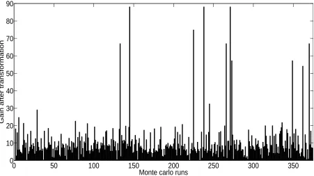
As can be seen in Fig. 1 the method that is introduced successfully removes the superharmonic as the gain index is very low (below one). However, as can be noted in Fig. 1, there are some few trials that SADE did not reach the global minimum. In contrast in Fig. 2 there is a confirmation of what was observed in the previous work. The 5th

order superharmonic is arising in magnitude to counter balance the reduction of the the 3rd

order superharmonic.

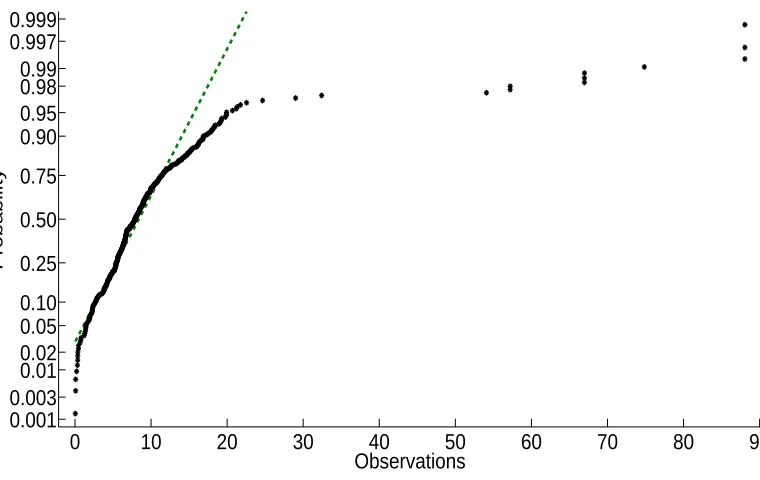
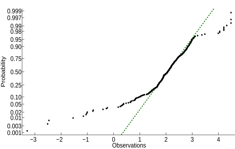
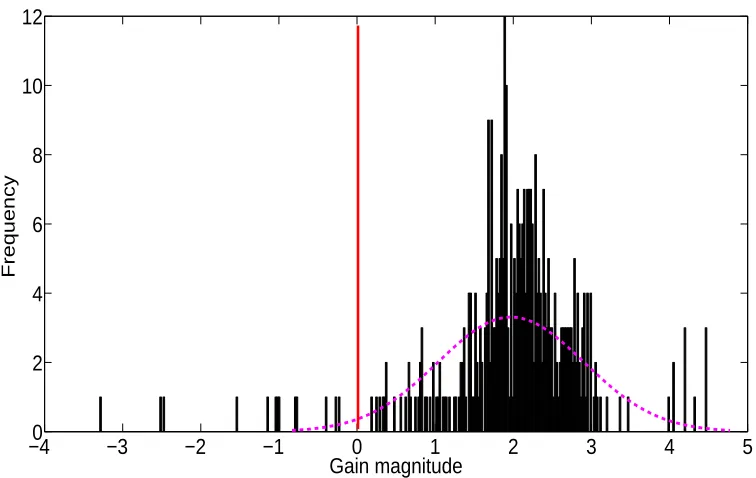
In Fig. 3 a normal test plot is used in order to investigate whether processed (transformed) data of the fifth harmonic exhibits the standard normal or Gaussian distribution. The green straight line gives the normal density function and one has to check the plotted points, and see how well they fit the normal line. In Fig. 3 the data points bend down and to the right of the green line which is an indication of a long tail to the left or left skew. This conclusion can also be seen in Fig. 4 where the histogram of the gain amplitude of the fifth order harmonic is presented.

The red line in Fig. 4 represents the threshold (gain value one) after which the gain of the fifth harmonic increases as result of minimising the third harmonic. It is very clear that the majority of the runs give gain magnitudes much higher that one. This confirms statistically what was expected via the simplifying transformation.

0

50

100

150

200

250

300

350

0

0.2

0.4

0.6

0.8

1

1.2

1.4

1.6

1.8

Gain after transformation

Monte carlo runs

Fig. 1: Gain of nonlinear system after transformation for the maximum amplitude of the third order harmonic.

0

50

100

150

200

250

300

350

0

10

20

30

40

50

60

70

80

90

Gain after transformation

Monte carlo runs

gain amplitude of the fifth order harmonic is presented and the normal density function is fitted (purple dotted line).

Again, the red line in Fig. 4 represents the threshold after (right) which the gain of the fifth harmonic increases as result of minimising the third harmonic. It is very clear that the majority of the runs give gain magnitudes much higher that one. Also, the data appears to be more Gaussian which could be proved useful in order to derive meaningful statistics.

0

10

20

30

40

50

60

70

80

90

0.001

0.003

0.01

0.02

0.05

0.10

0.25

0.50

0.75

0.90

0.95

0.98

0.99

0.997

0.999

Observations

Probability

0

5

10 15 20 25 30 35 40 45 50 55 60 65 70 75 80 85 90

0

2

4

6

8

10

12

14

16

18

Gain magnitude

Frequency

Fig. 4: Histogram of the maximum amplitude of the fifth order harmonic.

−3

−2

−1

0

1

2

3

4

0.001

0.003

0.01

0.02

0.05

0.10

0.25

0.50

0.75

0.90

0.95

0.98

0.99

0.997

0.999

Observations

Probability

−4

0

−3

−2

−1

0

1

2

3

4

5

2

4

6

8

10

12

Gain magnitude

Frequency

Fig. 6: Histogram of the maximum amplitude of the fifth order harmonic in the logarithmic scale.

4

Conclusion

The purpose of this paper is to highlight the key utility of some machine learning methods, not only for dynamic analysis of structure but as well as a method of simplification for nonlinear mechanical systems. The main benefit of the approach taken here is that complicated algebraic analysis is not necessary. Furthermore, the physical equations of the system are not needed. As a result, this machine learning approach is suited to experimental investigation of nonlinear systems using only the measured output responses. A further work is under preparation that deals with MDOF systems, where one attempts to remove interaction/combination frequencies from MDOF system responses. One might regard this as a means of decoupling the degrees of freedom.

Acknowledgments

The support of the UK Engineering and Physical Sciences Research Council (EPSRC) through grant reference number EP/J016942/1 and EP/K003836/2 is gratefully acknowledged.

References

[1] Keith Worden, Graeme Manson, Hoon Sohn, and CR Farrar. Extreme value statistics from differential evolution for damage detection. In Proceedings of the 23rd International Modal Analysis Conference (IMAC XXIII), pages 2009–3, 2005.

[2] Rainer Storn and Kenneth Price. Differential evolution–a simple and efficient heuristic for global optimization over continuous spaces. Journal of global optimization, 11(4):341–359, 1997.