On Lower and Upper Bounds in Smooth and Strongly Convex Optimization

On Lower and Upper Bounds in Smooth and Strongly

Convex Optimization

Yossi Arjevani [email protected]

Department of Computer Science and Applied Mathematics Weizmann Institute of Science

Rehovot 7610001, Israel

Shai Shalev-Shwartz [email protected]

School of Computer Science and Engineering The Hebrew University

Givat Ram, Jerusalem 9190401, Israel

Ohad Shamir [email protected]

Department of Computer Science and Applied Mathematics Weizmann Institute of Science

Rehovot 7610001, Israel

Editor:Mark Schmidt

Abstract

We develop a novel framework to study smooth and strongly convex optimization algo-rithms. Focusing on quadratic functions we are able to examine optimization algorithms as a recursive application of linear operators. This, in turn, reveals a powerful connection between a class of optimization algorithms and the analytic theory of polynomials whereby new lower and upper bounds are derived. Whereas existing lower bounds for this setting are only valid when the dimensionality scales with the number of iterations, our lower bound holds in the natural regime where the dimensionality is fixed. Lastly, expressing it as an optimal solution for the corresponding optimization problem over polynomials, as formulated by our framework, we present a novel systematic derivation of Nesterov’s well-known Accelerated Gradient Descent method. This rather natural interpretation of AGD contrasts with earlier ones which lacked a simple, yet solid, motivation.

Keywords: smooth and strongly convex optimization, full gradient descent, accelerated gradient descent, heavy ball method

1. Introduction

In the field of mathematical optimization one is interested in efficiently solving a minimiza-tion problem of the form

min

x∈Xf(x), (1)

even to approximate. As a consequence, various structural assumptions on the objective function and the constraints set, along with better-suited optimization algorithms, have been proposed so as to make this problem viable.

One such case is smooth and strongly convex functions over some d-dimensional Eu-clidean space1. Formally, we consider continuously differentiable f : Rd → R which are

L-smooth, i.e.,

k∇f(x)− ∇f(y)k ≤Lkx−yk, ∀x,y∈Rd, and µ-strongly convex, that is,

f(y)≥f(x) +hy−x,∇f(x)i+µ

2 ky−xk

2

, ∀x,y∈_Rd.

A wide range of applications together with very efficient solvers have made this family of problems very important. Naturally, an interesting question arises: how fast can these kind of problems be solved? better said, what is the computational complexity of minimizing smooth and strongly-convex functions to a given degree of accuracy?2 Prior to answering these, otherwise ill-defined, questions, one must first address the exact nature of the under-lying computational model.

Although being a widely accepted computational model in the theoretical computer sciences, the Turing Machine Model presents many obstacles when analyzing optimization algorithms. In their seminal work, Nemirovsky and Yudin (1983) evaded some of these difficulties by proposing the black box computational model, according to which informa-tion regarding the objective funcinforma-tion is acquired iteratively by querying an oracle. This model does not impose any computational resource constraints3. Nemirovsky and Yudin showed that for any optimization algorithm which employs a first-order oracle, i.e. receives (f(x),∇f(x)) upon querying at a pointx∈Rd, there exists anL-smoothµ-strongly convex quadratic function f :Rd →R, such that for any > 0 the number of oracle calls needed for obtaining an-optimal solution ˜x, i.e.,

f(˜x)< min

x∈_Rdf(x) +, (2)

must satisfy

# Oracle Calls≥Ω min˜ d,√κln(1/ , (3)

whereκ=M L/µdenotes the so-called condition number.

1. More generally, one may consider smooth and strongly convex functions over some Hilbert space. 2. Natural as these questions might look today, matters were quite different only few decades ago. In his

book ‘Introduction to Optimization’ which dates back to 87’, Polyak B.T devotes a whole section as to: ‘Why Are Convergence Theorems Necessary?’ (See section 1.6.2 in Polyak (1987)).

The result of Nemirovsky and Yudin can be seen as the starting point of the present paper. The restricted validity of this lower bound to the first O(d) iterations is not a mere artifact of the analysis. Indeed, from an information point of view, a minimizer of any convex quadratic function can be found using no more than O(d) first-order queries. Noticing that this bound is attained by the Conjugate Gradient Descent method (CGD, see Polyak 1987), it seems that one cannot get a non-trivial lower bound once the number of queries exceeds the dimension d. Moreover, a similar situation can be shown to occur for more general classes of convex functions. However, the known algorithms which attain such behavior (such as CGD and the center-of-gravity method, e.g., Nemirovski 2005) require computationally intensive iterations, and are quite different than many common algorithms used for large-scale optimization problems, such as gradient descent and its variants. Thus, to capture the attainable performance of such algorithms, we must make additional assump-tions on their structure. This can be made more solid using the following simple observation.

When applied on quadratic functions, the update rule of many optimization algorithms reduces to a recursive application of a linear transformation which depends, possibly ran-domly, on the previous p query points.

Indeed, the update rule of CGD for quadratic functions isnon-stationary, i.e. uses a different transformation at each iteration, as opposed to other optimization algorithms which utilize less complex update rules such as: stationary updates rule, e.g., Gradient Descent, Accel-erated Gradient Descent, Newton’s method (see Nesterov 2004), The Heavy Ball method Polyak (1987), SDCA (see Shalev-Shwartz and Zhang 2013) and SAG (see Roux et al. 2012); cyclic update rules, e.g,. SVRG (see Johnson and Zhang 2013); and piecewise-stationary update rules, e.g., Accelerated SDCA. Inspired by this observation, in the present work we explore the boundaries of optimization algorithms which admit stationary update rules. We call such algorithmsp-Stationary Canonical Linear Iterative optimization algorithms (abbr.

p-SCLI), where pdesignates the number of previous points which are necessary to generate new points. The quantity p may be instructively interpreted as a limit on the amount of memory at the algorithm’s disposal.

As eigenvalues are merely roots of characteristic polynomials4, our approach involves establishing a lower bound on the maximal modulus (absolute value) of the roots of poly-nomials. Clearly, in order to find a meaningful lower bound, one must first find a condition which is satisfied by all characteristic polynomials that correspond to p-SCLIs. We show that such condition does exist by proving that characteristic polynomials of consistent p -SCLIs, which correctly minimize the function at hand, must have a specific evaluation at

λ= 1. This in turn allows us to analyze the convergence rate purely in terms of the analytic theory of polynomials, i.e.,

Find min{ρ(q(z))|q(z) is a real monic polynomial of degreep and q(1) =r}, (4) where r ∈_R and ρ(q(z)) denotes the maximum modulus over all roots of q(z). Although a vast range of techniques have been developed for bounding the moduli of roots of poly-nomials (e.g., Marden 1966; Rahman and Schmeisser 2002; Milovanovic et al. 1994; Walsh 1922; Milovanovi´c and Rassias 2000; Fell 1980), to the best of our knowledge, few of them address lower bounds (see Higham and Tisseur 2003). Minimization problem (4) is also strongly connected with the question of bounding the spectral radius of ‘generalized’ com-panion matrices from below. Unfortunately, this topic too lacks an adequate coverage in the literature (see Wolkowicz and Styan 1980; Zhong and Huang 2008; Horne 1997; Huang and Wang 2007). Consequently, we devote part of this work to establish new tools for tack-ling (4). It is noteworthy that these tools are developed by using elementary arguments. This sharply contrasts with previously proof techniques used for deriving lower bounds on the convergence rate of optimization algorithms which employed heavy machinery from the field of extremal polynomials, such as Chebyshev polynomials (e.g., Mason and Handscomb 2002).

Based on the technique described above we present a novel lower bound on the conver-gence rate of p-SCLI optimization algorithms. More formally, we prove that any p-SCLI optimization algorithm overRd, whose iterations can be executed efficiently, requires

#Oracle Calls≥Ω˜ √p

κln(1/) (5)

in order to obtain an -optimal solution, regardless of the dimension of the problem. This result partially complements the lower bound presented earlier in Inequality (3). More specifically, for p = 1, we show that the runtime of algorithms whose update rules do not depend on previous points (e.g. Gradient Descent) and can be computed efficiently scales linearly with the condition number. For p = 2, we get the optimal result for smooth and strongly convex functions. For p > 2, this lower bound is clearly weaker than the lower bound shown in (3) at the first d iterations. However, we show that it can be indeed at-tained by p-SCLI schemes, some of which can be executed efficiently for certain classes of quadratic functions. Finally, we believe that a more refined analysis of problem (4) would show that this technique is powerful enough to meet the classical lower bound√κ for any

p, in the worst-case over all quadratic problems.

The last part of this work concerns a cornerstone in the field of mathematical optimiza-tion, i.e., Nesterov’s well-known Accelerated Gradient Descent method (AGD). Prior to the work of Nemirovsky and Yudin, it was known that full Gradient Descent (FGD) obtains an

-optimal solution by issuing no more than

O(κln(1/))

first-order queries. The gap between this upper bound and the lower bound shown in (3) has intrigued many researchers in the field. Eventually, it was this line of inquiry that led to the discovery of AGD by Nesterov (see Nesterov 1983), a slight modification of the standard GD algorithm, whose iteration complexity is

O √κln(1/).

Unfortunately, AGD lacks the strong geometrical intuition which accompanies many opti-mization algorithms, such as FGD and the Heavy Ball method. Primarily based on sophis-ticated algebraic manipulations, its proof strives for a more intuitive derivation (e.g. Beck and Teboulle 2009; Baes 2009; Tseng 2008; Sutskever et al. 2013; Allen-Zhu and Orecchia 2014). This downside has rendered the generalization of AGD to different optimization scenarios, such as constrained optimization problems, a highly non-trivial task which up to the present time does not admit a complete satisfactory solution. Surprisingly enough, by designing optimization algorithms whose characteristic polynomials are optimal with re-spect to a constrained version of (4), we have uncovered a novel simple derivation of AGD. This reformulation as an optimal solution for a constrained optimization problem over poly-nomials, shows that AGD and the Heavy Ball are essentially two sides of the same coin.

To summarize, our main contributions, in order of appearance, are the following:

• We define a class of algorithms (p-SCLI) in terms of linear operations on the last p

iterations, and show that they subsume some of the most interesting algorithms used in practice.

• We prove that any p-SCLI optimization algorithm must use at least

˜

Ω √p_κln(1/)

iterations in order to obtain an -optimal solution. As mentioned earlier, unlike ex-isting lower bounds, our bound holds for every fixed dimensionality.

• We show that there exist matchingp-SCLI optimization algorithms which attain the convergence rates stated above for allp. Alas, for p≥3, an expensive pre-calculation task renders these algorithms inefficient.

• We present new schemes which offer better utilization of second-order information by exploiting breaches in existing lower bounds. This leads to a new optimization algorithm which obtains a rate of √3_{κln(1/) in the presence of large enough spectral} gaps.

1.1 Notation

We denote scalars with lower case letters and vectors with bold face letters. We use R++ to denote the set of all positive real numbers. All functions in this paper are defined over Euclidean spaces equipped with the standard Euclidean norm and all matrix-norms are assumed to denote the spectral norm.

We denote a block-diagonal matrix whose blocks are A1, . . . , Ak by the conventional

direct sum notation, i.e., ⊕k

i=1Ak. We devote a special operator symbol for scalar matrices

Diag (a1, . . . , ad) = ⊕di=1ai. The spectrum of a square matrix A and its spectral radius,

the maximum magnitude over its eigenvalues, are denoted byσ(A) andρ(A), respectively. Recall that the eigenvalues of a square matrix A ∈ _Rd×d _{are exactly the roots of the}

characteristic polynomial which is defined as follows

χA(λ) = det(A−λId),

whereId denotes the identity matrix. Since polynomials in this paper have their origins as

characteristic polynomials of some square matrices, by a slight abuse of notation, we will denote the roots of a polynomial q(z) and its root radius, the maximum modulus over its roots, by σ(q(z)) andρ(q(z)), respectively, as well.

The following notation for quadratic functions and matrices will be of frequent use,

Sd(Σ)=M

n

A∈_Rd×d

A is symmetric andσ(A)⊆Σ o

,

Qd_(Σ)=M _{f A,b(x)

A∈ S

d_(Σ),b∈

Rd o

,

where Σ denotes a non-empty set of positive reals, and wherefA,b(x) denotes the following

quadratic function

fA,b(x)=M

1 2x

>_Ax+b>_{x, A∈ S}d_(Σ).

2. Framework

2.1 Case Study - Stochastic Dual Coordinate Ascent

We consider the optimization algorithm Stochastic Dual Coordinates Ascent (SDCA5) for solving Regularized Loss Minimization (RLM) problems (6), which are of great significance for the field of Machine Learning. It is shown that applying SDCA on quadratic loss func-tions allows one to reformulate it as a recursive application of linear transformafunc-tions. The relative simplicity of such processes is then exploited to derive a lower bound on the con-vergence rate.

A smooth-RLM problem is an optimization task of the following form:

min

w∈_RdP(w)

M

= 1

n n

X

i=1

φi(w>xi) + λ

2 kwk

2_{, (6)}

whereφi are 1/γ-smooth and convex, x1, . . . ,xn are vectors in Rd and λis a positive con-stant. For ease of presentation, we further assume that φi are non-negative, φi(0)≤1 and

kxik ≤1 for all i.

The optimization algorithm SDCA works by minimizing an equivalent optimization problem

min

α∈_RnD(α)

M

= 1

n n

X

i=1

φ?_i(αi) +

1 2λn2

n

X

i=1 αixi

2 ,

where φ? denotes the Fenchel conjugate of φ, by repeatedly picking z ∼ U([n]) uniformly and minimizingD(α) over thez’th coordinate. The latter optimization problem is referred to as the dual problem, while the problem presented in (6) is called theprimal problem. As shown in Shalev-Shwartz and Zhang (2013), it is possible to convert a high quality solution of the dual problem into a high quality solution of the primal problem. This allows one to bound from above the number of iterations required for obtaining a prescribed level of accuracy >0 by

˜ O

n+ 1

λγ

ln(1/)

.

We now show that this analysis is indeed tight. First, let us define the following 2-smooth functions:

φi(y) =y2, i= 1, . . . , n

and let us define x1=x2=· · ·=xn= √1_n1. This yields

D(α) = 1 2α

>

1 2nI+

1

λn211

>

α. (7)

Clearly, the unique minimizer ofD(α) isα∗ = 0. Now, givenM i∈[n] and α∈Rn, it is easy to verify that

argmin

α0_∈

R

D(α1, . . . , αi−1, α0, αi+1, . . . , αn) =

−2 2 +λn

X

j6=i

αj. (8)

Thus, the next test point α+, generated by taking a step along the i’th coordinate, is a linear transformation of the previous point, i.e.,

α+=I−eiu>i

α, (9)

where

u>_i =M





2

2 +λn, . . . ,

2

2 +λn, |{z}1

i’s entry

, 2

2 +λn, . . . ,

2 2 +λn



.

Let αk_{, k = 1, . . . , K denote the k’th test point. The sequence of points (α}k₎K

k=1 is

ran-domly generated by minimizing D(α) over thezi’th coordinate at thei’th iteration, where z1, z2, . . . , zK ∼ U([n]) is a sequence of K uniform distributed i.i.d random variables.

Ap-plying (9) over and over again starting from some initialization pointα0 _{we obtain}

αk =I−ezKu>zK I−ezK−1u >

zK−1

· · ·I−ez1u >

z1

α0.

To computeE[αK] note that by the i.i.d hypothesis and by the linearity of the expectation operator,

EαK=E

h

I−ezKu>_zK I−ezK−1u >

zK−1

· · ·I−ez1u > z1 α0 i =E h

I−ezKu>zK

i E

h

I−ezK−1u >

zK−1 i

· · ·_EhI−ez1u > z1 i α0 =E h

I−ezu>z

iK

α0. (10)

The convergence rate of the latter is governed by the spectral radius of

E=M E h

I−ezu>z

i

.

A straightforward calculation shows that the eigenvalues of E, ordered by magnitude, are

1− 1

2/λ+n, . . . ,1−

1 2/λ+n

| {z }

n−1 times

,1− 2 +λ

2 +λn. (11)

By choosingα0 to be the following normalized eigenvector which corresponds to the largest eigenvalue

α0=

1 √

2,− 1 √

2,0, . . . ,0

and plugging it into Equation (10), we can now bound from below the distance of E[αK] to the optimal point α∗ = 0,

E

αK−α∗= E

h

I −ezu>z

iK α0

=

1− 1

2/λ+n

K α0

=

1− 2

(4/λ+ 2n−1) + 1

K

≥

exp

₋

1 2/λ+n−1

K

,

where the last inequality is due to the following inequality,

1− 2

x+ 1 ≥exp

−2

x−1

, ∀x≥1. (12)

We see that the minimal number of iterations required for obtaining a solution whose distance from the α∗ is less than >0 must be greater than

(2/λ+n−1) ln (1/),

thus showing that, up to logarithmic factors, the analysis of the convergence rate of SDCA is tight.

2.2 Definitions

In the sequel we introduce the framework of p-SCLI optimization algorithms which gener-alizes the analysis shown in the preceding section.

We denote the set of d×d symmetric matrices whose spectrum lies in Σ ⊆ R++ by Sd_{(Σ) and denote the following set of quadratic functions}

fA,b(x)=M

1 2x

>_Ax+b>_{x, A∈ S}d_(Σ),

byQd_{(Σ). Note that since twice continuous differentiable functionsf(x) areL-smooth and} µ-strongly convex if and only if

σ ∇2_(f(x))

⊆[µ, L]⊆_R++_{, x∈}

Rd,

we have that Qd_{([µ, L]) comprisesL-smooth µ-strongly convex quadratic functions. Thus,}

any optimization algorithm designed for minimizing smooth and strongly convex functions can be used to minimize functions inQd_{([µ, L]). The key observation here is that since the}

gradient of fA,b(x) is linear in x, when applied to quadratic functions, the update rules of

Definition 1 (p-SCLI optimization algorithms) An optimization algorithmAis called a p-stationary canonical linear iterative (abbr. p-SCLI) optimization algorithm over Rd if

there exist p+ 1 mappings C0(X), C1(X), . . . , Cp−1(X), N(X) from Rd×d to Rd×d-valued

random variables, such that for any fA,b(x) ∈ Qd(Σ) the corresponding initialization and

update rules take the following form:

x0,x1, . . . ,xp−1∈_Rd (13)

xk=

p−1

X

j=0

Cj(A)xk−p+j+N(A)b, k=p, p+ 1, . . . (14)

We further assume that in each iteration Cj(A) and N(A) are drawn independently of previous realizations6, and that ECi(A) are finite and simultaneously triangularizable7.

Let us introduce a few more definitions and terminology which will be used throughout this paper. The number of previous pointspby which new points are generated is called the

lifting factor. The matrix-valued random variables C0(X), C1(X), . . . , Cp−1(X) and N(X)

are called coefficient matrices and inversion matrix, respectively. The term inversion ma-trix refers to the mapping N(X), as well as to a concrete evaluation of it. It will be clear from the context which interpretation is being used. The same holds for coefficient matrices.

As demonstrated by the following definition, coefficients matrices of p-SCLIs can be equivalently described in terms of polynomial matrices8. This correspondence will soon play a pivotal role in the analysis of p-SCLIs.

Definition 2 The characteristic polynomial of a given p-SCLI optimization algorithmAis defined by

LA(λ, X)=M Idλp− p−1

X

j=0

ECj(X)λj, (15)

where Cj(X) denote the coefficient matrices. Moreover, given X∈Rd×d we define the root

radius ofLA(λ, X) by

ρλ(LA(λ, X)) =ρ(detLA(λ, X)) = max

|λ0|

detLA(λ0, X) = 0 .

For the sake of brevity, we sometimes specify a given p-SCLI optimization algorithm A using an ordered pair of a characteristic polynomial and an inversion matrix as follows

A= (M LA(λ, X), N(X)).

Furthermore, we may omit the subscript A, when it is clear from the context.

6. We shall refer to this assumption asstationarity.

7. Intuitively, having this technical requirement is somewhat similar to assuming that the coefficients ma-trices commute (see Drazin et al. 1951 for a precise statement), and as such does not seem to restrict the scope of this work. Indeed, it is common to have ECi(A) as polynomials in Aor as diagonal matrices,

in which case the assumption holds true.

Lastly, note that nowhere in the definition ofp-SCLIs did we assume that the optimiza-tion process converges to the minimizer of the funcoptimiza-tion under consideraoptimiza-tion - an assumpoptimiza-tion which we refer to as consistency.

Definition 3 (Consistency of p-SCLI optimization algorithms) Ap-SCLI optimiza-tion algorithmAis said to be consistent with respect to a givenA∈ Sd_{(Σ)if for anyb∈}

Rd, A converges to the minimizer of fA,b(x), regardless of the initialization point. That is, for

xk∞

k=1 as defined in (13,14) we have that

xk→ −A−1b,

for anyb∈Rd. Furthermore, if Ais consistent with respect to all A∈ Sd(Σ), then we say

thatA is consistent with respect to Qd_(Σ).

2.3 Specifications for Some Popular Optimization Algorithms

Having defined the framework of p-SCLI optimization algorithms, a natural question now arises: how broad is the scope of this framework and what does characterize optimization algorithms which it applies to? Loosely speaking, any optimization algorithm whose update rules depend linearly on the first and the second order derivatives of the function under con-sideration is eligible for this framework. Instead of providing a precise characterization for such algorithms, we apply various popular optimization algorithms on a general quadratic functionfA,b(x)∈ Qd([µ, L]) and then express them asp-SCLI optimization algorithms.

Full Gradient Descent (FGD) is a 1-SCLI optimization algorithm with

x0 ∈_Rd_,

xk+1 =xk−β∇f(xk) =xk−β(Axk+b) = (I −βA)xk−βb,

β = 2

µ+L.

See Nesterov (2004) for more details.

Newton method is a 0-SCLI optimization algorithm with

x0∈_Rd_,

xk+1=xk−(∇2f(xk))−1∇f(xk) =xk−A−1(Axk+b) = (I−A−1A)xk−A−1b=−A−1b.

Note that Newton method can be also formulated as a degenerate p-SCLI for some

The Heavy Ball Method is a 2-SCLI optimization algorithm with

xk+1 =xk−α∇f(xk) +β(xk−xk−1) =xk−α(Axk+b) +β(xk−xk−1) = ((1 +β)I−αA)xk−βIxk−1−αb,

α= 4

√

L+õ2

, β = √

L−√µ

√

L+õ

!2

.

See Polyak (1987) for more details.

Accelerated Gradient Descent (AGD) is a 2-SCLI optimization algorithm with

x0 =y0 ∈_Rd, yk+1 =xk− 1

L∇f(x k_),

xk+1 = (1 +α)yk+1−αyk, α =

√

L−√µ

√

L+õ,

which can be rewritten as follows:

x0 ∈_Rd, xk+1 = (1 +α)

xk− 1

L∇f(x k₎

−α

xk−1− 1

L∇f(x k−1₎

= (1 +α)

xk− 1

L(Ax k_+b)

−α

xk−1− 1

L(Ax

k−1_+b)

= (1 +α)

I− 1

LA

xk−α

I− 1

LA

xk−1− 1

Lb.

Note that here we employ a stationary variant of AGD. See Nesterov (2004) for more details.

Stochastic Coordinate Descent (SCD) is a 1-SCLI optimization algorithm. This is a generalization of the example shown in Section 2.1. SCD acts by repeatedly minimiz-ing a uniformly randomly drawn coordinate in each iteration. That is,

x0∈Rd,

Picki∼ U([d]) and set xk+1=

I− 1

Ai,i eia>_i,?

xk− bi

Ai,i ei,

wherea>_i,? denotes the i’th row of Aand b = (M b1, b2, . . . , bd). Note that the expected

update rule of this method is equivalent to the well-known Jacobi’s iterative method.

Conjugate Gradient Descent (CGD) can be expressed as a non-stationary iterative method

xk+1 = ((1 +βk)I −αkA)xk−βkIxk−1−αkb,

where αk and βk are computed at each iteration based on xk,xk−1, A and b. Note

the similarity of CGD and the heavy ball method. See Polyak (1987); Nemirovski (2005) for more details. In the context of this framework, CGD forms the ‘most non-stationary’ kind of method in that its coefficientsαk, βkare highly dependent on time

and the function at hand.

Stochastic Gradient Descent (SGD) A straightforward extension of the deterministic FGD. Specifically, let (Ω,F,P) be a probability space and letG(x, ω) :Rd×Ω→Rd be an unbiased estimator of∇f(x) for any x. That is,

E[G(x, ω)] =∇f(x) =Ax+b, x∈Rd.

Equivalently, definee(x, ω) =G(x, ω)−(Ax+b) and assumeE[e(x, ω)] = 0, x∈Rd. SGD may be defined using a suitable sequence of step sizes (γi)∞i=1 as follows:

Generateωk randomly and setxk+1 =xk−γiG(xk, ωk)

= (I−γiA)xk−γib−γie(x, ω).

Clearly, some types of noise may not form ap-SCLI optimization algorithm. However, for some instances, e.g., quadratic learning problems, we have

e(x, ω) =Aωx+bω,

such that

E[Aω] = 0, E[bω] = 0.

If, in addition, the step size is fixed then we get a 1-SCLI optimization algorithm. See Kushner and Yin (2003); Spall (2005); Nemirovski (2005) for more details.

2.4 Computational Complexity

The stationarity property of generalp-SCLIs optimization algorithms implies that the com-putational cost of minimizing a given quadratic function fA,b(x), assuming Θ (1) cost for

all arithmetic operations, is

# Iterations × 

 

 

Generating coefficient and inversion matrices randomly +

Executing update rule (14) based on the previousppoints

randomly generating coefficient and inversion matrices each time. Notice that for determin-isticp-SCLIs one can save running time by computing the coefficient and inversion matrices once, prior to the execution of the algorithm. Not surprisingly, but interesting nonethe-less, there is a law of conservation which governs the total amount of computational cost invested in both factors: the more demanding is the task of randomly generating coefficient and inversion matrices, the less is the total number of iterations required for obtaining a given level of accuracy, and vice versa. Before we can make this statement more rigorous, we need to present a few more facts about p-SCLIs. For the time being, let us focus on theiteration complexity, i.e., the total number iterations, which forms our analogy for black box complexity.

The iteration complexity of a p-SCLI optimization algorithm A with respect to an ac-curacy level , initialization points X0 _{and a quadratic function f}

A,b(x), symbolized by

ICA , fA,b(x),X0

,

is defined to be the minimal number of iterationsK such that

E[x

k_−x∗_]

< , ∀k≥K,

wherex∗ =−A−1b is the minimizer offA,b(x), assumingA is initialized atX0. We would

like to point out that although iteration complexity is usually measured through

E x

k_−x∗ ,

here we employ a different definition. We will discuss this issue shortly.

In addition to showing that the iteration complexity of p-SCLI algorithms scales log-arithmically with 1/, the following theorem provides a characterization for the iteration complexity in terms of the root radius of the characteristic polynomial.

Theorem 4 LetAbe ap-SCLI optimization algorithm overRdand letfA,b(x)∈ Qd(Σ), (Σ⊆

R++) be a quadratic function. Then, there existsX0∈(Rd)p such that ICA , fA,b(x),X0

= ˜Ω

ρ

1−ρln(1/)

,

and for all X0 _∈(

Rd)p, it holds that

ICA , fA,b(x),X0

= ˜O

1

1−ρln(1/)

,

where ρ denotes the root radius of the characteristic polynomial evaluated atX =A.

• First, we express update rule (14) as a single step rule by introducing new variables in some possibly higher-dimensional Euclidean space (Rd)p,

z0 = x0,x1, . . . ,xp−1>

∈_Rpd, zk =M(X)zk−1+U N(X)b, k= 1,2, . . .

Recursively applying this rule and taking expectation w.r.t the coefficient matrices and the inversion matrix yields

E h

zk−z∗i=E[M]k(z0−z∗).

• Then, to derive the lower bound, we use the Jordan form ofE[M] to show that there exists some non-zero vectorr∈(Rd)p such that ifhz0−z∗,ri 6= 0, then kE[M]k(z0−

z∗)k is asymptotically bounded from below by some geometric sequence. The upper bound follows similarly.

• Finally, we express the bound on the convergence rate of (zk) in terms of the original space.

Carefully inspecting the proof idea shown above reveals that the lower bound remains valid even in cases where the initialization points are drawn randomly. The only condition for this to hold is that the underlying distribution is reasonable, in the sense that it is absolutely continuous w.r.t. the Lebesgue measure, which implies that Pr[hz0−z∗,ri 6= 0] = 1.

We remark that the constants in the asymptotic behavior above may depend on the quadratic function under consideration, and that the logarithmic terms depend on the dis-tance of the initialization points from the minimizer, as well as the lifting factor and the spectrum of the Hessian. For the sake of clarity, we omit the dependency on these quantities.

There are two, rather subtle, issues regarding the definition of iteration complexity which we would like to address. First, observe that in many cases a given point ˜x∈_Rd_{is said to}

be-optimal w.r.t some real functionf :Rd→R if

f(˜x)< min

x∈_Rdf(x) +.

However, here we employ a different measure for optimality. Fortunately, in our case either can be used without essentially affecting the iteration complexity. That is, although in general the gap between these two definitions can be made arbitrarily large, for L-smooth

µ-strongly convex functions we have

µ

2 kx−x ∗_k2_≤

f(x)−f(x∗)≤ L

2 kx−x ∗_k2

.

Secondly, here we measure the sub-optimality of the k’th iteration by E[xk−x∗] ,

whereas in many other stochastic settings it is common to derive upper and lower bounds on Exk−x∗

. That being the case, by

E

x

k_−x∗

2

=E

x

k₋

Exk

2

+

E

h

xk−x∗

i

2 ,

we see that if the variance of the k’th point is of the same order of magnitude as the norm of the expected distance from the optimal point, then both measures are equivalent. Consequently, our upper bounds imply upper bounds on E

h

xk−x∗

2i

for deterministic algorithms (where the variance term is zero), and our lower bounds imply lower bounds

on E h

xk−x∗

2i

, for both deterministic and stochastic algorithms (since the variance is non-negative). We defer a more adequate treatment for this matter to future work.

3. Deriving Bounds for p-SCLI Algorithms

The goal of the following section is to show how the framework of p-SCLI optimization algorithms can be used to derive lower and upper bounds. Our presentation follows from the simplest setting to the most general one. First, we present a useful characterization of consistency (see Definition 3) of p-SCLIs using the characteristic polynomial. Next, we demonstrate the importance of consistency through a simplified one dimensional case. This line of argument is then generalized to any finite dimensional space and is used to explain the role of the inversion matrix. Finally, we conclude this section by providing a schematic description of this technique for the most general case which is used both in Section (4) to establish lower bounds on the convergence rate ofp-SCLIs with diagonal inversion matrices, and in Section (5) to derive efficientp-SCLIs.

3.1 Consistency

Closely inspecting various specifications for p-SCLI optimization algorithms (see Section (2.3)) reveals that the coefficient matrices always sum up to I +EN(X)X, where N(X) denotes the inversion matrix. It turns out that this is not a mere coincidence, but an extremely useful characterization for consistency of p-SCLIs. To see why this condition must hold, supposeAis a deterministicp-SCLI algorithm overRdwhose coefficient matrices and inversion matrix areC0(X), . . . , Cp−1(X) andN(X), respectively, and suppose that A

is consistent w.r.t some A ∈ Sd_{(Σ). Recall that every p+ 1 consecutive points generated}

by Aare related by (14) as follows

xk=

p−1

X

j=0

Cj(A)xk−p+j+N(A)b, k=p, p+ 1, . . .

Taking limit of both sides of the equation above and noting that by consistency

for any b∈_Rd_{, yields}

−A−1b=−

p−1

X

j=0

Cj(A)A−1b+N(A)b.

Thus,

−A−1=−

p−1

X

j=0

Cj(A)A−1+N(A).

Multiplying by A and rearranging, we obtain

p−1

X

j=0

Cj(A) =Id+N(A)A. (16)

On the other hand, if instead of assuming consistency we assume thatAgenerates a conver-gent sequence of points and that Equation (16) holds, then the arguments used above show that the limit point must be−A−1_{b. In terms of the characteristic polynomial ofp-SCLIs,}

this formalized as follows.

Theorem 5 (Consistency via Characteristic Polynomials) Suppose A = (M L(λ, X)

, N(X)) is a p-SCLI optimization algorithm. Then, A is consistent with respect to A ∈ Sd_{(Σ) if and only if the following two conditions hold:}

1.L(1, A) =−_EN(A)A (17)

2. ρλ(L(λ, A))<1 (18)

The proof for the preceding theorem is provided in Section C.2. This result will be used extensively throughout the reminder of this work.

3.2 Simplified One-Dimensional Case

To illustrate the significance of consistency in the framework of p-SCLIs, consider the fol-lowing simplified case. Suppose A is a deterministic 2-SCLI optimization algorithm over Q1_{([µ, L]), such that its inversion matrix N(x) is some constant scalar ν ∈}

R and its co-efficient matrices c0(x), c1(x) are free to take any form. The corresponding characteristic

polynomial is

L(λ, x) =λ2−c1(x)λ−c0(x).

Now, let fa,b(x) ∈ Q1([µ, L]) be a quadratic function. By Theorem 4, we know that A

converges to the minimizer offa,b(x) with an asymptotic geometric rate of ρλ(L(λ, a)), the

maximal modulus root. Thus, ideally we would like to set cj(x) = 0, j = 0,1. However,

this might violate the consistency condition (17), according to which, one must maintain

That being the case, how little canρλ(L(λ, a)) be over all possible choices for cj(a) which

satisfyL(1, a) =−νa? Formally, we seek to solve the following minimization problem

ρ∗ = min{ρλ(L(λ, a)) | L(λ, a) is a real monic quadratic polynomial in λand L(1) =−νa}.

By consistency we also have that ρ∗ must be strictly less than one. This readily implies that−νa >0. In which case, Lemma 6 below gives

ρ∗ ≥ρ

λ−1−√−νa2= √

−νa−1. (19)

The key observation here is that ν cannot be chosen so as to be optimal for allQ1_{([µ, L])}

simultaneously. Indeed, the preceding inequality holds in particular for a=µ and a=L, by which we conclude that

ρ∗≥max

n

√

−νµ−1,

√

−νL−1

o

≥ √

κ−1 √

κ+ 1, (20)

where κ =M L/µ. Plugging in Inequality (20) into Theorem 4 implies that there exists

fa,b(x)∈ Q1([µ, L]) such that the iteration complexity ofA for minimizing it is

˜ Ω

√

κ−1

2 ln(1/)

.

To conclude, by applying this rather natural line of argument we have established a lower bound on the convergence rate of any 2-SCLI optimization algorithms for smooth and strongly convex function overR, e.g., AGD and HB.

3.3 The General Case and the Role of the Inversion Matrix

We now generalize the analysis shown in the previous simplified case to any deterministic

p-SCLI optimization algorithm over any finite dimensional space. This generalization relies on a useful decomposability property of the characteristic polynomial, according to which deriving a lower bound on the convergence rate of p-SCLIs overRd is essentially equivalent for derivingdlower bounds on the maximal modulus of the roots of dpolynomials overR.

Let A= (M L(λ, X), N(X)) be a consistent deterministic p-SCLI optimization algorithm and letfA,b(x)∈ Qd(Σ) be a quadratic function. By consistency (see Theorem 5) we have

L(1, A) =−N A

(for brevity we omit the functional dependency on X). Since coefficient matrices are as-sumed to be simultaneously triangularizable, there exists an invertible matrix Q ∈ _Rd×d

such that

Tj =M Q−1CjQ, j = 0,1, . . . , p−1

are upper triangular matrices. Thus, by the definition of the characteristic polynomial (Definition 2) we have

detL(λ, X) = det Q−1L(λ, X)Q= det



Idλp− p−1

X

j=0 Tjλj



=

d

Y

j=1

where

`j(λ) =λp− p−1

X

k=0

σ_jkλk, (22)

and whereσ₁j, . . . , σ_dj, j = 0, . . . , p−1 denote the elements on the diagonal ofTj, or

equiv-alently the eigenvalues ofCj ordered according toQ. Hence, the root radius of the

charac-teristic polynomial of Ais

ρλ(L(λ, X)) = max{|λ| |`i(λ) = 0 for some i∈[d]}. (23)

On the other hand, by consistency condition (17) we get that for alli∈[d],

`i(1) =σi(L(1)) =σi(−N A). (24)

It remains to derive a lower bound on the maximum modulus of the roots of`i(λ), subject

to constraint (24). To this end, we employ the following lemma whose proof can be found in Section C.3.

Lemma 6 Suppose q(z) is a real monic polynomial of degree p. If q(1)<0, then

ρ(q(z))>1.

Otherwise, if q(1)≥0, then

ρ(q(z))≥

p

p

q(1)−1

.

In which case, equality holds if and only if

q(z) =z−(1−pp

q(1))p.

We remark that the second part of Lemma 6 implies that subject to constraint (24), the lower bound stated above is unimprovable. This property is used in Section 5 where we aim to obtain optimal p-SCLIs by designing `j(λ) accordingly. Clearly, in the presence of

additional constraints, one might be able to improve on this lower bound (see Section 4.2).

Since Ais assumed to be consistent, Lemma 6 implies thatσ(−N(A)A)⊆R++, as well as the following lower bound on the root radius of the characteristic polynomial,

ρλ(L(λ, X))≥max i∈[d]

p

p

σi(−N(A)A)−1

. (25)

Noticing that the reasoning above can be readily applied to stochasticp-SCLI optimization algorithms, we arrive at the following corollary which combines Theorem 4 and Inequality (25).

Corollary 7 Let A be a consistent p-SCLI optimization algorithm with respect to some

A∈ Sd_{(Σ), let N(X) denote the corresponding inversion matrix and let}

ρ∗ = max

i∈[d]

p

p

σi(−EN(A)A)−1 ,

then the iteration complexity ofA for any fA,b(x)∈ Qd(Σ)is lower bounded by

˜ Ω

ρ∗

1−ρ∗ ln(1/)

Using Corollary 7, we are now able to provide a concise ‘plug-and-play’ scheme for deriving lower bounds on the iteration complexity of p-SCLI optimization algorithms. To motivate this scheme, note that the effectiveness of the lower bound stated in Corollary 7 is directly related to the magnitude of the eigenvalues of −N(X)X. To exemplify this, consider the inversion matrix of Newton method (see Section 2.3)

N(X) =−X−1.

Since

σ(−N(X)X) ={1},

the lower bound stated above is meaningless for this case. Nevertheless, the best computa-tional cost for computing the inverse ofd×dregular matrices known today is super-quadratic ind. As a result, this method might become impractical in large scale scenarios where the dimension of the problem space is large enough. A possible solution is to employ inversion matrices whose dependence on X is simpler. On the other hand, if N(X) approximates −X−1 very badly, then the root radius of the characteristic polynomial might get too large. For instance, if N(X) = 0 then

σ(−N(X)X) ={0},

contradicting the consistency assumption, regardless of the choice of the coefficient matrices.

In light of the above, many optimization algorithms can be seen as strategies for bal-ancing the computational cost of obtaining a good approximation for the inverse ofX and executing large number of iterations. Put differently, various structural restrictions on the inversion matrix yield different σ(−N(X)X), which in turn lead to a lower bound on the root radius of the corresponding characteristic polynomial. This gives rise to the following scheme:

Scheme 1 Lower bounds

Parameters: • A family of quadratic functionsQd_(Σ)

• An inversion matrixN(X) • A lifting factorp∈_N,

Choose S0 _{⊆ S}d_(Σ)

Verify ∀A∈ S0, σ(−EN(A)A)⊆(0,2p) to ensure consistency (Theorem 5)

Bound max

A∈S0_,i∈[d]

p

p

σi(−EN(A)A)−1

from below by some ρ∗ ∈[0,1)

Lower bound: Ω˜

ρ∗

1−ρ∗ln(1/)

This scheme is implicitly used in the previous Section (3.2), where we established a lower bound on the convergence rate of 2-SCLI optimization algorithms over R with constant inversion matrix and the following parameters

Σ = [µ, L], S0 ={µ, L}.

3.4 Bounds Schemes

In spite of the fact that Scheme 1 is expressive enough for producing meaningful lower bounds under various structures of the inversion matrix, it does not allow one to incorpo-rate other lower bounds on the root radius of characteristic polynomials whose coefficient matrices admit certain forms, e.g., linear coefficient matrices (see 35 below). Abstracting away from Scheme 1, we now formalize one of the main pillar of this work, i.e., the relation between the amount of computational cost one is willing to invest in executing each itera-tion and the total number of iteraitera-tions needed for obtaining a given level of accuracy. We use this relation to form two schemes for establishing lower and upper bounds forp-SCLIs.

Given a compatible set of parameters: a lifting factorp, an inversion matrixN(X), set of quadratic functionsQd_{(Σ) and a set of coefficients matricesC, we denote byA(p, N(X),Q}d_(Σ),C)

the set of consistent p-SCLI optimization algorithms for Qd_{(Σ) whose inversion matrix}

are N(X) and whose coefficient matrices are taken from C. Furthermore, we denote by

L(p, N(X),Qd_{(Σ),C) the following set of polynomial matrices}







L(λ, X)=M Idλp− p−1

X

j=0

ECj(X)λj

Cj(X)∈ C, L(1, A) =−N(A)A, ∀A∈ Sd(Σ)







.

Since both sets are determined by the same set of parameters, the specifications of which will be occasionally omitted for brevity. The natural one-to-one correspondence between these two set, as manifested by Theorem 4 and Corollary 5, yields

min

A∈A fA,b(maxx)∈Qd(Σ)

ρλ(LA(λ, A)) = min

L(λ,X)∈L Amax∈Sd_(Σ)ρλ(L(λ, A)) (27)

The importance of Equation (27) stems from its ability to incorporate any bound on the maximal modulus root of polynomial matrices into a general scheme for bounding the iteration complexity ofp-SCLIs. This is summarized by the following scheme.

Scheme 2 Lower bounds

Given a set of p-SCLI optimization algorithmsA(p, N(X),Qd_(Σ),C) Find ρ∗ ∈[0,1) such that

min

L(λ,X)∈L Amax∈Sd_(Σ)ρλ(L(λ, A))≥ρ∗ Lower bound: Ω˜ ρ∗

1−ρ∗ln(1/)

Scheme 3 Optimal p-SCLI Optimization Algorithms

Given a set of polynomial matrices L(p, N(X),Qd_(Σ),C)

Compute ρ∗ = min

L(λ,X)∈L A∈Smaxd_(Σ)ρλ(L(λ, A))

and denote its minimizer by L∗_{(λ, A)}

Upper bound: The corresponding p-SCLI algorithm for L∗(λ, A)

Convergence rate: O₁₋1_ρ∗ln(1/)

4. Lower Bounds

In the sequel we derive lower bounds on the convergence rate ofp-SCLI optimization algo-rithms whose inversion matrices are scalar or diagonal, and discuss the assumptions under which these lower bounds meet matching upper bounds. It is likely that this approach can be also effectively applied for block-diagonal inversion, as well as for a much wider set of inversion matrices whose entries depend on a relatively small set of entries of the matrix to be inverted.

4.1 Scalar and Diagonal Inversion Matrices

We derive a lower bound on the convergence rate of p-SCLI optimization algorithms for

L-smoothµ-strongly convex functions overRdwith a scalar inversion matrix N(X) by em-ploying Scheme 1 (see Section 3.3). Note that since the one-dimensional case was already proven in Section 3.2, we may assume thatd≥2.

First, we need to pick a ‘hard’ matrix inSd_{([µ, L]). It turns out that any positive-definite}

matrixA∈ Sd_{([µ, L]) for which}

{µ, L} ⊆σ(A), (28)

will meet this criterion. For the sake of concreteness, let us define

A= Diag(M L, µ, . . . , µ

| {z }

d−1 times

).

In which case,

−ν{µ, L}=σ(−_EN(A)A),

whereνI =E[N(A)]. Thus, to maintain consistency, it must hold that9

ν ∈

₋

2p

L ,0

. (29)

Next, to bound from below

ρ∗ = maxM

i∈[d]

p

p

σi(−νA)−1

= max n

|√p_{−νµ−1|,|}√p

−νL−1|o,

we split the feasible range of ν (29) into three different sub-ranges as follows:

p

√

−νµ−1<0 √p_{−νµ−1≥0}

Case 1 N/A

p

√

−νL−1≤0 Range: [−1/L,0) Minimizer: ν∗=−1/L

Lower bounds: 1−qp µ L

Case 2 Case 3 (requires: p≥log₂κ)

p

√

−νL−1>0 Range: (−1/µ,−1/L) Range: (−2p/L,−1/µ] Minimizer: −√p 2

L+√p_µ

p

Minimizer: −1/µ

Lower bound:

p

√

L/µ−1 p

√

L/µ+1 Lower Bound: p

q

L µ −1

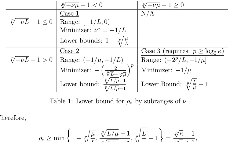
Table 1: Lower bound for ρ∗ by subranges ofν

Therefore,

ρ∗ ≥min

(

1− p

r

µ L,

p

p

L/µ−1

p

p

L/µ+ 1,

p

s

L µ −1

)

=

p

√

κ−1

p

√

κ+ 1, (30)

where κ =M L/µ, upper bounds the condition number of functions in Qd_{([µ, L]). Thus, by}

Scheme 1, we get the following lower bound on the worse-case iteration complexity,

˜ Ω

√p_κ−1

2 ln(1/)

. (31)

As for the diagonal case, it turns out that for any quadraticfA,b(x)∈ Qd([µ, L]) which has

L+µ

2

L−µ 2 L−µ

2

L+µ 2

(32)

as a principal sub-matrix of A, the best p-SCLI optimization algorithm with a diagonal inversion matrix does not improve on the optimal asymptotic convergence rate achieved by scalar inversion matrices (see Section C.4). Overall, we obtain the following theorem.

Theorem 8 Let Abe a consistent p-SCLI optimization algorithm forL-smoothµ-strongly convex functions over Rd. If the inversion matrix of A is diagonal, then there exists a

quadratic function fA,b(x)∈ Qd([µ, L]) such that

ICA(, fA,b(x)) = ˜Ω

√p_κ−1

2 ln(1/)

, (33)

4.2 Is This Lower Bound Tight?

A natural question now arises: is the lower bound stated in Theorem 8 tight? In short, it turns out that for p = 1 and p = 2 the answer is positive. For p > 2, the answer heavily depends on whether a suitable spectral decomposition is within reach. Obviously, computing the spectral decomposition for a given positive definite matrix A is at least as hard as finding the minimizer of a quadratic function whose Hessian is A. To avoid this, we will later restrict our attention to linear coefficients matrices which allow efficient implementation.

A matching upper bound for p= 1 In this case the lower bound stated in Theorem 8 is simply attained by FGD (see Section 2.3).

A matching upper bound for p= 2 In this case there are two 2-SCLI optimization al-gorithm which attain this bound, namely, Accelerated Gradient Descent and The Heavy Ball method (see Section 2.3), whose inversion matrices are scalar and corre-spond to Case 1 and Case 2 in Table 1, i.e.,

NHB=−

2 √

L+õ

!2

Id, NAGD=

−1

L Id.

Although HB obtains the best possible convergence rate in the class of 2-SCLIs with diagonal inversion matrices, it has a major disadvantage. When applied to general smooth and strongly-convex functions, one cannot guarantee global convergence. That is, in order to converge to the corresponding minimizer, HB must be initialized close enough to the minimizer (see Section 3.2.1 in Polyak 1987). Indeed, if the initialization point is too far from the minimizer then HB may diverge as shown in Section 4.5 in Lessard et al. (2014). In contrast to this, AGD attains a global linear convergence with a slightly worse factor. Put differently, the fact HB is highly adapted to quadratic functions prevents it from converging globally to the minimizers of general smooth and strongly convex functions.

A matching upper bound for p >2 In Subsection A we show that when no restriction on the coefficient matrices is imposed, the lower bound shown in Theorem 8 is tight, i.e., for anyp∈_Nthere exists a matchingp-SCLI optimization algorithm with scalar inversion matrix whose iteration complexity is

˜

O √p_κln(1/)

. (34)

In light of the existing lower bound which scales according to√κ, this result may seem surprising at first. However, there is a major flaw in implementing these seemingly ideal p-SCLIs. In order to compute the corresponding coefficients matrices one has to obtain a very good approximation for the spectral decomposition of the positive definite matrix which defines the optimization problem. Clearly, this approach is rarely practical. To remedy this situation we focus on linear coefficient matrices which admit a relatively low computational cost per iteration. That is, we assume that there exist real scalars α1, . . . , αp−1 and β1, . . . , βp−1 such that

We believe that for these type of coefficient matrices the lower bound derived in Theorem 8 is not tight. Precisely, we conjecture that for any 0< µ < L and for any consistentp-SCLI optimization algorithmAwith diagonal inversion matrix and linear coefficients matrices, there existsfA,b(x)∈ Qd([µ, L]) such that

ρλ(LA(λ, X))≥

√

κ−1 √

κ+ 1,

where κ =M L/µ. Proving this may allow to derive tight lower bounds for many optimization algorithm in the field of machine learning. Using Scheme 2, which allows to incorporate various lower bounds on the root radius of polynomials, one is able to equivalently express this conjecture as follows: suppose q(z) is ap-degree monic real polynomial such thatq(1) = 0. Then, for any polynomialr(z) of degree p−1 and for any 0< µ < L, there existsη∈[µ, L] such that

ρ(q(z)−ηr(z))≥ p

L/µ−1

p

L/µ+ 1.

That being so, can we do better if we allow families of quadratic functions Qd_(Σ)

where Σ are not necessarily continuous intervals? It turns out that the answer is positive. Indeed, in Section B we present a 3-SCLI optimization algorithm with linear coefficient matrices which, by being intimately adjusted to quadratic functions whose Hessian admits large enough spectral gap, beats the lower bound of Nemirovsky and Yudin (3). This apparently contradicting result is also discussed in Section B, where we show that lower bound (3) is established by employing quadratic functions whose Hessian admits spectrum which densely populates [µ, L].

5. Upper Bounds

Up to this point we have projected various optimization algorithms on the framework of

p-SCLI optimization algorithms, thereby converting questions on convergence properties into questions on moduli of roots of polynomials. In what follows, we shall head in the opposite direction. That is, first we define a polynomial (see Definition (2)) which meets a prescribed set of constraints, and then we form the corresponding p-SCLI optimization algorithm. As stressed in Section 4.2, we will focus exclusively on linear coefficient matrices which admit low per-iteration computational cost and allow a straightforward extension to general smooth and strongly convex functions. Surprisingly enough, this allows a systematic recovering of FGD, HB, AGD, as well as establishing new optimization algorithms which allow better utilization of second-order information. This line of inquiry is particularly important due to the obscure nature of AGD, and further emphasizes its algebraic char-acteristic. We defer stochastic coefficient matrices, as in SDCA, (Section 2.1) to future work.

5.1 Linear Coefficient Matrices

In the sequel we instantiate Scheme 3 (see Section 3.4) forC_Linear, the family of deterministic linear coefficient matrices.

First, note that due to consistency constraints, inversion matrices of constant p-SCLIs with linear coefficient matrices must be either constant scalar matrices or else be com-putationally equivalent to A−1. Therefore, since our motivation for resorting to linear coefficient matrices was efficiency, we can safely assume that N(X) = νId for some ν ∈

(−2p/L,0). Following Scheme 3, we now seek the optimal characteristic polynomial in

LLinear =M L(p, νId,Qd([µ, L]),CLinear) with a compatible set of parameters (see Section 3.4).

In the presence of linearity, the characteristic polynomials takes the following simplified form

L(λ, X) =λp−

p−1

X

j=0

(ajX+bjId)λj, aj, bj ∈R.

By (23) we have

ρλ(L(λ, X)) = max{|λ| | ∃i∈[d], `i(λ) = 0},

where`i(λ) denote the factors of the characteristic polynomial as in (22). That is, denoting

the eigenvalues ofX byσ1, . . . , σdwe have

`i(λ) =λp− p−1

X

j=0

(ajσi+bj)λj =λp−σi p−1

X

j=0

ajλj+ p−1

X

j=0 bjλj.

Thus, we can express the maximal root radius of the characteristic polynomial overQd_{([µ, L])}

in terms of the following polynomial

`(λ, η) =λp−(ηa(λ) +b(λ)), (36)

for some real univariate p−1 degree polynomials a(λ) and b(λ), whereby

max

A∈Sd_(Σ)ρλ(L(λ, A)) = max_η∈[µ,L]ρ(`(λ, η)).

That being the case, finding the optimal characteristic polynomial in LLinear translates to

the following minimization problem,

minimize

`(λ,η)∈LLinear max

η∈[µ,L]ρλ(`(λ, η))

s.t. `(1, η) =−νη, η∈[µ, L] (37)

ρλ(`(λ, η))<1 (38)

(Note that in this case we think ofLLinearas a set of polynomials whose variable assumes

This optimization task can be readily solved for the setting where the lifting factor is

p= 1, the family of quadratic functions under considerations isQd_{([µ, L]) and the inversion}

matrix is N(X) =νId, ν∈(−2/L,0). In which case (36) takes the following form

`(λ, η) =λ−ηa0−b0,

where a0, b0 are some real scalars. In order to satisfy (37) for all η ∈ [µ, L], we have no

other choice but to set

a0=ν, b0 = 1,

which implies

ρλ(`(λ, η)) = 1 +νη.

Since ν ∈(−2/L,0), condition 38 follows, as well. The corresponding 1-SCLI optimization algorithm is

xk+1= (I+νA)xk+νb,

and its first-order extension (see Section 5.3 below) is precisely FGD (see Section 2.3). Finally, note that the corresponding root radius is bounded from above by

κ−1

κ

forν =−1/L, the minimizer in Case 2 of Table 1, and by

κ−1

κ+ 1

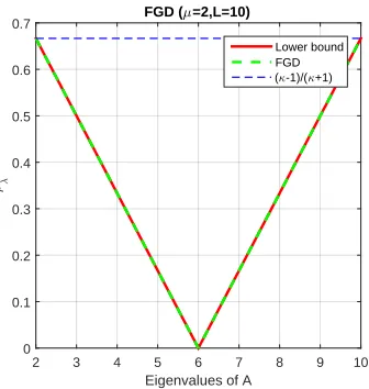
for ν = _µ+L−2 , the minimizer in Case 3 of Table 1. This proves that FGD is optimal for the class of 1-SCLIs with linear coefficient matrices. Figure 5.1 shows how the root radius of the characteristic polynomial of FGD is related to the eigenvalues of the Hessian of the quadratic function under consideration.

5.2 Recovering AGD and HB

Let us now calculate the optimal characteristic polynomial for the setting where the lifting factor isp= 2, the family of quadratic functions under considerations is Qd_{([µ, L]) and the}

inversion matrix isN(X) =νId, ν ∈(−4/L,0) (recall that the restricted range of ν is due

to consistency). In which case (36) takes the following form

`(λ, η) =λ2−η(a1λ+a0)−(b1λ+b0), (39)

for some real scalars a0, a1, b0, b1. Our goal is to choose a0, a1, b0, b1 so as to minimize

max

Eigenvalues of A

2 3 4 5 6 7 8 9 10

;6

0 0.1 0.2 0.3 0.4 0.5 0.6

0.7 FGD (7=2,L=10)

Lower bound FGD (5-1)/(5+1)

Figure 1: The root radius of FGD vs. various eigenvalues of the corresponding Hessian.

while preserving conditions (37) and (38). Note that `(λ, η), when seen as a function of

η, forms a linear path of quadratic functions. Thus, a natural way to achieve this goal is to choose `(λ, η) so that `(λ, µ) and `(λ, L) take the form of the ‘economic’ polynomials introduced in Lemma 6, namely

λ−(1−√r)2

for r = −νµ and r = −νL, respectively, and hope that for others η ∈ (µ, L), the roots of

`(λ, η) would still be of small magnitude. Note that due to the fact that`(λ, η) is linear in

η, condition (37) readily holds for anyη∈(µ, L). This yields the following two equations

`(λ, µ) =

λ−(1−p−νµ)

2

,

`(λ, L) =λ−(1−p−νL)2.

Substituting (39) for`(λ, η) and expanding the r.h.s. of the equations above we get

λ2−(a1µ+b1)λ−(a0µ+b0) =λ2−2(1−

√

−νµ)λ+ (1−√−νµ)2, λ2−(a1L+b1)λ−(a0L+b0) =λ2−2(1−

√

−νL)λ+ (1−√−νL)2.

Which can be equivalently expressed as the following system of linear equations

−(a1µ+b1) =−2(1−

√

−νµ), (40)

−(a0µ+b0) = (1−

√

−νµ)2, (41)

−(a1L+b1) =−2(1−

√

−νL), (42)

−(a0L+b0) = (1−

√

Eigenvalues of A

2 3 4 5 6 7 8 9 10

;6

0 0.1 0.2 0.3 0.4 0.5

0.6 AGD (7=2,L=10)

Lower bound AGD ( 5-1)/ 5

Eigenvalues of A

2 3 4 5 6 7 8 9 10

;6

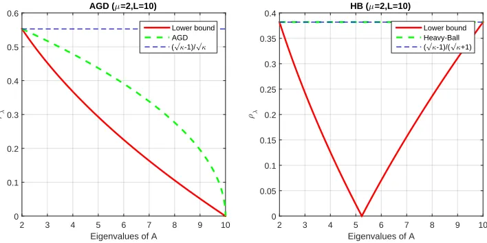
0 0.05 0.1 0.15 0.2 0.25 0.3 0.35

0.4 HB (7=2,L=10)

Lower bound Heavy-Ball ( 5-1)/( 5+1)

Figure 2: The root radius of AGD and HB vs. various eigenvalues of the corresponding Hessian.

Multiplying Equation (40) by -1 and add to it Equation (42). Next, multiply Equation (41) by -1 and add to it Equation (43) yields

a1(µ−L) = 2

√

−ν(√L−√µ),

a0(µ−L) = (1−

√

−νL)2−(1−√−νµ)2.

Thus,

a1=

−2√−ν

√

µ+√L, a0 =

2√−ν

√

µ+√L +ν.

Plugging in ν = −1/L (see Table 1) into the equations above and solving for b1 and b0

yields a 2-SCLI optimization algorithm whose extension (see Section 5.3 below) is precisely AGD. Following the same derivation only this time by setting (see again Table 1)

ν =− √ 2

L+õ

!2

yields the Heavy-Ball method .

Moreover, using standard formulae for roots of quadratic polynomials one can easily verify that

ρλ(`(λ, η))≤

√

κ−1 √

κ , η∈[µ, L],

for AGD, and

ρλ(`(λ, η))≤

√

κ−1 √

for HB. In particular, Condition 38 holds. Figure 5.2 shows how the root radii of the char-acteristic polynomials of AGD and HB are related to the eigenvalues of the Hessian of the quadratic function under consideration.

Unfortunately, finding the optimal p-SCLIs for p > 2 is open and is closely related to the conjecture presented in the end of Section 4.2.

5.3 First-Order Extension for p-SCLIs with Linear Coefficient Matrices

As mentioned before, since the coefficient matrices of p-SCLIs can take any form, it is not clear how to use a given p-SCLI algorithm, efficient as it may be, for minimizing general smooth and strongly convex functions. That being the case, one could argue that recov-ering the specifications of, say, AGD for quadratic functions does not necessarily imply how to recover AGD itself. Fortunately, consistent p-SCLIs with linear coefficients can be reformulated as optimization algorithms for general smooth and strongly convex functions in a natural way by substituting ∇f(x) for Ax+b, while preserving the original conver-gence properties to a large extent. In the sequel we briefly discuss this appealing property, namely, canonical first-order extension, which completes the path from the world of polyno-mials to the world optimization algorithm for general smooth and strongly convex functions.

LetA= (M LA(λ, X), N(X)) be a consistentp-SCLI optimization algorithm with a scalar inversion matrix, i.e.,N(X)=M νId, ν ∈(−2p/L,0), and linear coefficient matrices

Cj(X) =ajX+bjId, j= 0, . . . , p−1, (44)

wherea0, . . . , ap−1∈Rand b0, . . . , bp−1 ∈Rdenote real scalars. Recall that by consistency, for any fA,b(x)∈ Qd(Σ), it holds that

p−1

X

j=0

Cj(A) =I+νA.

Thus,

p−1

X

j=0

bj = 1 and p−1

X

j=0

aj =ν. (45)

By the definition ofp-SCLIs (Definition 1), we have that

xk=C0(A)xk−p+C1(A)xk−(p−1)+· · ·+Cp−1(A)xk−1+νb.

Substituting Cj(A) for (44), gives

xk= (a0A+b0)xk−p+ (a1A+b1)xk−(p−1)+· · ·+ (ap−1A+bp−1)xk−1+νb.

Rearranging and plugging in 45, we get

xk=a0(Axk−p+b) +a1(Axk−(p−1)+b) +· · ·+ap−1(Axk−1+b)

Finally, by substituting Ax+b for its analog ∇f(x), we arrive at the following canonical first-order extension of A

xk=

p−1

X

j=0

bjxk−(p−j)+ p−1

X

j=0

aj∇f(xk−(p−j)). (46)

Being applicable to a much wider collection of functions, how well should we expect the canonical extensions to behave? The answer is that when initialized close enough to the minimizer, one should expect a linear convergence of essentially the same rate. A formal statement is given by the theorem below which easily follows from Theorem 1 in Section 2.1, Polyak (1987) for

g(xk−p,xk−(p−1), . . . ,xk−1) =

p−1

X

j=0

bjxk−(p−j)+ p−1

X

j=0

aj∇f(xk−(p−j)).

Theorem 9 Suppose f : Rd → R is an L-smooth µ-strongly convex function and let x∗

denotes its minimizer. Then, for every >0, there exist δ >0 and C >0 such that if

xj−x∗

≤δ, j= 0, . . . , p−1,

then

x

k_−x0 ≤C(ρ

∗₊₎k_{, k=p, p+ 1, . . . ,}

where

ρ∗ = sup

η∈Σ ρ



λp−

p−1

X

j=0

(ajη+bj)λj



.

Unlike generalp-SCLIs with linear coefficient matrices which are guaranteed to converge only when initialized close enough to the minimizer, AGD converges linearly, regardless of the initialization points, for any smooth and strongly convex function. This fact merits further investigation as to the precise principles which underlie p-SCLIs of this kind.

Appendix A. Optimal p-SCLI for Unconstrained Coefficient Matrices

In the sequel we use Scheme 3 (see Section 3.4) to show that, when no constraints are imposed on the functional dependency of the coefficient matrices, the lower bound shown in Theorem 8 is tight. To this end, recall that in Lemma 6 we showed that the lower bound on the maximal modulus of roots of a polynomials which evaluate at z = 1 to somer ≥0 is uniquely attained by the following polynomial

q_r∗(z)=M z−(1−√p_r)p

Concretely, let p∈_Nbe some lifting factor, let N(X) =νId, ν∈(−2p/L,0) be a fixed

scalar matrix and letfA,b(x)∈ Qd(Σ) be some quadratic function. Lemma 6 implies that

for each η ∈σ(−νA) we need the corresponding factor of the characteristic polynomial to be

`j(λ) = (λ−(1− p

√

η))p

=

p

X

k=0

p k

p

√

−νη−1p−k

λk (47)

This is easily accomplished using the spectral decomposition of A by

Λ=M U>AU

whereU is an orthogonal matrix and Λ is a diagonal matrix. Note that sinceAis a positive definite matrix such a decomposition must always exist. We define p coefficient matrices

C0, C1, . . . , Cp−1 in accordance with Equation (47) as follows

Ck=U



    

− p_k √_p

−νΛ11−1

p−k

− p_k √p₋

νΛ22−1

p−k

. ..

− p_k √_p

−νΛdd−1

p−k 

    

U>.

By using Theorem 5, it can be easily verified that these coefficient matrices form a consistent

p-SCLI optimization algorithm whose characteristic polynomial’s root radius is

max

j=1,...,d

p

p

−νµj−1

.

Choosing

ν =− 2

p

√

L+√p_µ

!p

according to Table 1, produces an optimal p-SCLI optimization algorithm for this set of parameters. It is noteworthy that other suitable decompositions can be used for deriving optimalp-SCLIs, as well.

As a side note, since the cost of computing each iteration in ∈_Rpd _{grows linearly with}

Appendix B. Lifting Factor ≥ 3

In Section 4.2 we conjecture that for anyp-SCLI optimization algorithmA= (M L(λ, X), N(X)), with diagonal inversion matrix and linear coefficient matrices there exists someA∈ Qd_{([µ, L])}

such that

ρλ(L(λ, X))≥

√

κ−1 √

κ+ 1, (48)

where κ =M L/µ. However, it may be possible to overcome this barrier by focusing on a subclass of Qd_{([µ, L]). Indeed, recall that the polynomial analogy of this conjecture states}

that for any monic realpdegree polynomialq(z) such thatq(1) = 0 and for any polynomial

r(z) of degreep−1, there existsη ∈[µ, L] such that

ρ(q(z)−ηr(z))≥ √

κ−1 √

κ+ 1.

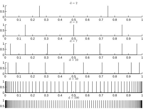
This implies that we may be able to tune q(z) and r(z) so as to obtain a convergence rate, which breaks Inequality (48), for quadratic function whose Hessian’s spectrum does not spread uniformly across [µ, L].

Let us demonstrate this idea for p= 3, µ = 2 and L= 100. Following the exact same derivation used in the last section, let us pick

q(z, η)=M zp−(ηa(z) +b(z))

numerically, so that

q(z, µ) =z−(1−p3

−νµ)3

q(z, L) =

z−(1−p3 −νµ)

3

where

ν =− 2

3 √

L+√3_µ !3

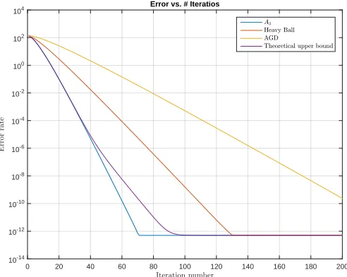
The resulting 3-CLI optimization algorithmA3 is

xk=C2(X)xk−1+C1(X)xk−2+C0(X)xk−3+N(X)b

where

C0(X)≈0.1958Id−0.0038X C1(X)≈ −0.9850Id