A Bounded
p
-norm Approximation of Max-Convolution for
Sub-Quadratic Bayesian Inference on Additive Factors
Julianus Pfeuffer
Eberhard Karls Universit¨at T¨ubingen
Oliver Serang [email protected]
Freie Universit¨at Berlin Department of Informatik
Takustr. 9, 14195 Berlin, Germany
and
The Leibniz-Institute of Freshwater Ecology and Inland Fisheries (IGB) M¨uggelsee 310, 12587 Berlin, Germany
Editor:Amos Storkey
Abstract
Max-convolution is an important problem closely resembling standard convolution; as such, max-convolution occurs frequently across many fields. Here we extend the method with fastest known worst-case runtime, which can be applied to nonnegative vectors by numerically approximating the Chebyshev normk · k∞, and use this approach to derive two numerically stable methods based
on the idea of computingp-norms via fast convolution: The first method proposed, with runtime inO(klog(k) log(log(k))) (which is less than 18klog(k) for any vectors that can be practically re-alized), uses thep-norm as a direct approximation of the Chebyshev norm. The second approach proposed, with runtime inO(klog(k)) (although in practice both perform similarly), uses a novel null space projection method, which extracts information from a sequence ofp-norms to estimate the maximum value in the vector (this is equivalent to querying a small number of moments from a distribution of bounded support in order to estimate the maximum). Thep-norm approaches are compared to one another and are shown to compute an approximation of the Viterbi path in a hidden Markov model where the transition matrix is a Toeplitz matrix; the runtime of approxi-mating the Viterbi path is thus reduced fromO(nk2) steps toO(nklog(k)) steps in practice, and is demonstrated by inferring the U.S. unemployment rate from the S&P 500 stock index.
Keywords: Bayesian inference,maximum a posteriori, fast Fourier transform, max-convolution,
p-norm,Lpspace, hidden Markov model, null space projection, polynomial matrix
1. Introduction
Max-convolution can be defined using vectors (or discrete random variables, whose probability mass functions are analogous to nonnegative vectors) with the relationshipM =L+R. Given the target sumM =m, the max-convolution finds the largest valueL[`]×R[r] for whichm=`+r.
M[m] = max
`,r:m=`+rL[`]R[r]
= max
` L[`]R[m−`] = (L ∗max R) [m]
where ∗max denotes the max-convolution operator. In probabilistic terms, this is equivalent to
finding the highest probability of the joint events Pr(L = `, R = r) that would produce each possible value of the sumM =L+R (note that in the probabilistic version, the vector M would subsequently need to be normalized so that its sum is 1).
Although applications of max-convolution are numerous, only a small number of methods exist for solving it (Serang, 2015). These methods fall into two main categories, each with their own draw-backs: The first category consists of very accurate methods that are have worst-case runtimes either quadratic (Bussieck et al., 1994) or slightly more efficient than quadratic in the worst-case (Brem-ner et al., 2006). Conversely, the second type of method computes a numerical approximation to the desired result, but inO(klog2(k)) steps; however, no bound for the numerical accuracy of this
method has been derived (Serang, 2015).
While the two approaches from the first category of methods for solving max-convolution do so by either using complicated sorting routines or by creating a bijection to an optimization problem, the numerical approach solves max-convolution by showing an equivalence between ∗max and the process of first generating a vectoru(m)for each indexmof the result (whereu(m)[`] =L[`]R[m−`]
for all in-bounds indices) and subsequently computing the maximum M[m] = max`u(m)[`]. When
L andR are nonnegative, the maximization over the vectoru(m) can be computed exactly via the
Chebyshev norm
M[m] = max
` u
(m)[`]
= lim
p→∞ku (m)
kp
but requiresO(k2) steps (wherekis the length of vectorsLandR). However, once a fixedp∗-norm
is chosen, the approximation corresponding to thatp∗ can be computed by expanding the p∗-norm to yield
lim p→∞ku
(m)k
p = lim
p→∞
X
`
u(m)[`] p!
1 p
≈ X
`
u(m)[`] p∗!
1 p∗
= X
`
L[`]p∗ R[m−`]p∗ !p1∗
= X
`
Lp∗[`]Rp∗[m−`] !p1∗
= Lp∗ ∗ Rp∗ 1 p∗
where Lp∗ = h (L[0])p∗
,(L[1])p∗, . . . , (L[k−1])p∗ i and ∗ denotes standard convolution. The standard convolution can be done via fast Fourier transform (FFT) inO(klog2(k)) steps, which is substantially more efficient than theO(k2) required by the naive method (Algorithm 1).
To date, the numerical method has demonstrated the best speed-accuracy trade-off on Bayesian inference tasks, and can be generalized to multiple dimensions (i.e., tensors). In particular, they have been used with probabilistic convolution trees (Serang, 2014) to efficiently compute the most probable values of discrete random variablesX0, X1, . . . Xn−1for which the sum is knownX0+X1+ . . . Xn−1=y (Serang, 2014). The one-dimensional variant of this problem (i.e., where eachXi is a one-dimensional vector) solves the probabilistic generalization of the subset sum problem, while the two-dimensional variant (i.e., where eachXi is a one-dimensional matrix) solves the generalization of the knapsack problem (note that these problems are not NP-hard in this specific case, because we assume an evenly-spaced discretization of the possible values of the random variables).
However, despite the practical performance that has been demonstrated by the numerical method, only cursory analysis has been performed to formalize the influence of the value ofp∗on the accuracy of the result and to bound the error of the p∗-norm approximation. Optimizing the choice of p∗
is non-trivial: Larger values of p∗ more closely resemble a true maximization under the p∗-norm,
but result in underflow (note that in Algorithm 1, the maximum values of bothLand R can be divided out and then multiplied back in after max-convolution so that overflow is not an issue). Conversely, smaller values of p∗ suffer less underflow, but compute a norm with less resemblance to maximization. Here we perform an in-depth analysis of the influence of p∗ on the accuracy of numerical max-convolution, and from that analysis we construct a modified piecewise algorithm, on which we demonstrate bounds on the worst-case absolute error. This modified algorithm, which runs in O(klog(k) log(log(k))) steps, is demonstrated using a hidden Markov model describing the relationship between U.S. unemployment and the S&P 500 stock index.
We then extend the modified algorithm and introduce a second modified algorithm, which not only uses a single p-norm as a means of approximating the Chebyshev norm, but instead uses a sequence ofp-norms and assembles them using a projection as a means to approximate the Chebyshev norm. Using numerical simulations as evidence, we make a conjecture regarding the relative error of the null space projection method. In practice, this null space projection algorithm is shown to have similar runtime and higher accuracy when compared with the piecewise algorithm.
2. Methods
We begin by outlining and comparing three numerical methods for max-convolution. By analyzing the benefits and deficits of each of these methods, we create improved variants. All of these methods will make use of the basic numerical max-convolution idea summarized in the introduction, and as such we first declare a method for computing the numerical max-convolution estimate for a given
p∗as numericalMaxConvolveGivenPStar(Algorithm 1).
Algorithm 1 Numerical max-convolution given a fixed p∗, a numerical method to estimate the max-convolution of two PMFs or nonnegative vectors. The parameters are two nonnegative vectors L0 and R0 (both scaled so that they have maximal element 1) and the numerical value p∗
used for computation. The return value is a numerical estimate of the max-convolutionL0 ∗max R0.
1: procedurenumericalMaxConvolveGivenPStar(L0,R0,p∗)
2: ∀`, vL[`]←L[`]p∗
3: ∀r, vR[r]←R[r]p∗
4: vM←vL ∗ vR .Standard FFT convolution is used here
5: ∀m, M0[m]←vM[m]p1∗
6: returnM0
2.1 Fixed Low-Value p∗= 8 Method:
The effects of underflow will be minimal (as it is not very far from standard FFT convolution, an operation with high numerical stability), but it can still be imprecise due to numerical “bleed-in” (i.e., error due to contributions from non-maximal terms for a given u(m) because the p∗-norm is
not identical to the Chebyshev norm). Overall, this will perform well on indices where the exact value of the result is small, but perform poorly when the exact value of the result is large.
2.2 Fixed High-Valuep∗= 64Method:
As noted above, will offer the converse pros and cons compared to using a lowp∗: numerical artifacts due to bleed-in will be smaller (thus achieving greater performance on indices where the exact values of the result are larger), but underflow may be significant (and therefore, indices where the exact results of the max-convolution are small will be inaccurate).
2.3 Higher-Order Piecewise Method:
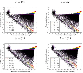
The higher-order piecewise method formalizes the empirical cutoff values found in Serang 2015; previously, numerical stability boundaries were found for eachp∗ by computing both the exact max-convolution (via the naiveO(k2) method) and via the numerical method using the ascribed value of p∗, and finding the value below which the numerical values experienced a high increase in relative absolute error.
Those previously observed empirical numerical stability boundaries can be formalized by using the fact that the employednumpyimplementation of FFT convolution has high accuracy on indices where the result has a value≥τ relative to the maximum value; therefore, if the argumentsLandR
are both normalized so that each has a maximum value of 1, the fast max-convolution approximation is numerically stable for any indexmwhere the result of the FFT convolution,i.e.,vM[m], is≥τ.
Thenumpydocumentation defines a conservative numeric tolerance for underflowτ= 10−12, which
is a conservative estimate of the numerical stability boundary demonstrated in Figure 1 (those boundary points occur very close to the true machine precision≈10−15).
Because Cooley-Tukey implementations of FFT-based convolution (e.g., thenumpy implementa-tion) are widely applied to large problems with extremely small error, we will make a simplification and assume that, when constraining the FFT result to reach a value higher than machine epsilon (+ tolerance threshold), the error from the FFT is negligible in comparison to the error introduced by thep∗-norm approximation. This is firstly because the only source of numerical error during FFT (assuming an FFT implementation with numerically precise twiddle factors) on vectors in [0,1]k will be the result of underflow from repeated addition and subtraction (neglecting the non-influencing multiplication with twiddle factors, which each have magnitude 1). The numerically imprecise rou-tines are thus limited to (x+y)−x; whenx >> y(i.e., yx < ≈10−15, the machine precision), then (x+y)−xwill return 0 instead ofy. To recover at least one bit of the significand, the intermediate results of the FFT must surpass machine precision(since the worst case addition initially happens with the maximumx= 1.0).
Figure 1: Empirical estimate of τ to construct a piecewise method. For each k ∈ {128,256,512,1024}, 32 replicate max-convolutions (on vectors filled with uniform values) are performed. Error from two sources can be seen: error due to underflow is depicted in the sharp left mode, whereas error due to imperfect approximation, wherek · kp∗>k · k∞
can be seen in the gradual mode on the right. Error due top∗-norm approximation is sig-nificantly smaller whenp∗is larger (thereby flattening the right mode), but largerp∗values
are more susceptible to underflow, pushing more indices into the left mode. Regardless of the value ofk, error due to underflow occurs when (k · kp∗)p
∗
goes below≈10−15; this is approximately the numerical tolerance for τ described by the numpy documentation. Therefore, at each index m we can construct a piecewise method that uses the largest value of p∗ for which the FFT convolution result is not close to the machine precision (i.e., (ku(m)k
p∗)p ∗
(e.g., k = 1024 as shown in Figure 1), it is empirically demonstrated that the influence of the length on the τ threshold is negligible. By using a numerical toleranceτ = 10−12, we ensure that the vast majority of numerical error for the numerical max-convolution algorithm is due to the p∗ -norm approximation (i.e., employing ku(m)kp∗ instead ofku(m)k∞) and not due to the long-used
and numerically performant FFT result. Furthermore, in practice the mean squared error due to FFT will be much smaller than the conservative worst-case outlined here, because it is difficult for the largest intermediate summed value (in this casex) to be consistently large when many such very small values (in this casey) are encountered in the same list. Althoughτcould be chosen specifically for a problem of sizek, note that this simple derivation is very conservative and thus it would be better to use a tighter bound for choosingτ. Regardless, for an FFT implementation that isn’t as performant (e.g., because it usesfloattypes instead ofdouble), increasingτ slightly would suffice. Therefore, from this point forward we consider that the dominant cause of error to come from the max-convolution approximation. Using larger p∗ values will provide a closer approximation; however, using a larger value ofp∗ may also drive values to zero (because the inputsL andR will be normalized withinAlgorithm 1 so that the maximum of each is 1 when convolved via FFT), limiting the applicability of largep∗ to indicesmfor whichvM[m]≥τ.
Through this lens, the choice ofp∗can be characterized by two opposing sources of error: higher
p∗ values better approximate ku(m)kp∗ but will be numerically unstable for many indices; lower p∗ values provide worse approximations ofku(m)kp∗ but will be numerically unstable for only few
indices. These opposing sources of error pose a natural method for improving the accuracy of this max-convolution approximation. By considering a small collection ofp∗values, we can compute the full numerical estimate (at all indices) with eachp∗ usingAlgorithm 1; computing the full result
at a given p∗ is∈O(klog2(k)), so doing so on some small number c of p∗ values considered, then the overall runtime will be ∈ O(cklog2(k)). Then, a final estimate is computed at each index by using the largest p∗ that is stable (with respect to underflow) at that index. Choosing the largest
p∗(of those that are stable with respect to underflow) corresponds to minimizing the bleed-in error, because the largerp∗ becomes, the more muted the non-maximal terms in the norm become (and thus the closer thep∗-norm becomes to the true maximum).
Here we introduce this piecewise method and compare it to the simpler low-value p∗ = 8 and high-valuep∗= 64 methods and analyze the worst-case error of the piecewise method.
3. Results
This section derives theoretical error bounds as well as a practical comparison on an example for the standard piecewise method. Furthermore the development of an improvement with affine scaling is shown. Eventually, an evaluation of the latter is performed on a larger problem. Therefore we applied our technique to compute the Viterbi path for a hidden Markov model (HMM) to assess runtime and the level of error propagation.
3.1 Error and Runtime Analysis of the Piecewise Method
We first analyze the error for a particular underflow-stablep∗ and then use that to generalize to the piecewise method, which seeks to use the highest underflow-stablep∗.
3.1.1 Error Analysis for a Fixed Underflow-Stablep∗:
We first scaleLandRintoL0 andR0 respectively, where the maximum elements of bothL0 andR0
are 1; the absolute error can be found by unscaling the absolute error of the scaled problem:
|exact(L, R)[m]−numeric(L0, R0)[m]|
= max
` L[`] maxr R[r]|exact(L
Algorithm 2 Piecewise numerical max-convolution , a numerical method to estimate the max-convolution of nonnegative vectors (revised to reduce bleed-in error). This procedure uses a
p∗ close to the largest possible stable value at each result index. The return value is a numerical estimate of the max-convolutionL∗maxR. The runtime is inO(klog2(k) log2(p∗max)).
1: procedurenumericalMaxConvolvePiecewise(L,R,p∗max)
2: `max←argmax`L[`]
3: rmax←argmaxrR[r]
4: L0← L L[`max]
5: R0← R
R[rmax] .Scale to a proportional problem onL
0
, R0
6: allP Star←[20,21, . . . ,2
log2(p∗max)
]
7: fori∈ {0,1, . . . len(allP Star)}do
8: resF orAllP Star[i]←fftNonnegMaxConvolveGivenPStar(L0,R0,allP Star[i])
9: end for
10: form∈ {0,1, . . . len(L) +len(R)−1}do
11: maxStableP StarIndex[m]←max{i: (resF orAllP Star[i][m])allPStar[i]≥τ)}
12: end for
13: form∈ {0,1, . . . len(L) +len(R)−1}do
14: i←maxStableP StarIndex[m]
15: result[m]←resF orAllP Star[i][m]
16: end for
17: returnL[`max]×R[rmax]×result .Undo previous scaling
18: end procedure
We first derive an error bound for the scaled problem onL0, R0 (any mention of a vectoru(m) refers
to the scaled problem), and then reverse the scaling to demonstrate the error bound on the original problem onL, R.
For any particular “underflow-stable” p∗ (i.e., any value of p∗ for which ku(m)k
p∗
p∗
≥ τ), the absolute error for the numerical method for fast max-convolution can be bound fairly easily by factoring out the maximum element ofu(m) (this maximum element is equivalent to the Chebyshev
norm) from thep∗-norm:
|exact(L0, R0)[m]−numeric(L0, R0)[m]|
= |ku(m)kp∗− ku(m)k∞|
= ku(m)kp∗− ku(m)k∞
= ku(m)k∞
ku(m)k
p∗ ku(m)k
∞ −1
= ku(m)k∞
k u (m)
ku(m)k∞kp∗−1
= ku(m)k∞kv(m)kp∗−1
wherev(m)is a nonnegative vector of the same length asu(m)(this length is denotedk
m) where
definition of the maximum). These observations result in the equation
kv(m)kp∗ ≤ k(1,1, . . .1)kp∗
= km
X
i 1p∗
!p1∗
= km
1 p∗.
Thus, sincekv(m)k
p∗≥1, the error is bounded:
|exact(L0, R0)[m]−numeric(L0, R0)[m]|
= ku(m)k∞
kv(m)kp∗−1
≤ kv(m)kp∗−1 ≤ k
1 p∗
m −1,
because∀m, ku(m)k∞≤1 for a scaled problem onL0, R0.
3.1.2 Error Analysis of Piecewise Method
However, the bounds derived above are only applicable forp∗ where ku(m)kp∗
p∗ ≥τ. The piecewise
method is slightly more complicated, and can be partitioned into two cases: In the first case, the top contour is used (i.e., whenp∗max is underflow-stable). Conversely, in the second case, a middle contour is used (i.e., when p∗max is not underflow-stable). In this context, in general a contour comprises of a set of indicesmwith the same maximum stablep∗.
In the first case, when we use the top contourp∗=p∗max, we know thatp∗maxmust be underflow-stable, and thus we can reuse the bound given an underflow-stablep∗.
In the second case, because the p∗ used is< p∗max, it follows that the next higher contour (using 2p∗) must not be underflow-stable (because the highest underflow-stablep∗ is used and because the
p∗are searched in log-space). The bound derived above that demonstrated
ku(m)kp∗≤ ku(m)k∞k 1 p∗
m
can be combined with the property thatk · kp∗≥ k · k∞ for anyp∗≥1 to show that
ku(m)k∞∈
"
ku(m)k
p∗
k 1 p∗
m
,ku(m)kp∗
#
.
Thus the absolute error can also be shown to be bounded using the fact that we are in a middle contour:
= ku(m)kp∗− ku(m)k∞
= ku(m)kp∗
1−ku
(m)k ∞ ku(m)k
p∗
≤ ku(m)kp∗
1−k
−1 p∗
m
< τ2p1∗
1−k
−1 p∗
m
The absolute error from middle contours will be quite small when p∗ = 1 is the maximum underflow-stable value of p∗ at index m, because τ21p∗, the first factor in the error bound, will
become√τ≈10−6, and 1−k −1 p∗
m <1 (qualitatively, this indicates that a smallp∗ is only used when the result is very close to zero, leaving little room for absolute error). Likewise, when a very large
p∗is used, then 1−k −1 p∗
m becomes very small, whileτ
1
2p∗ <1 (qualitatively, this indicates that when
a largep∗ is used, thek · kp∗ ≈ k · k∞, and thus there is little absolute error). Thus for the extreme
values ofp∗, middle contours will produce fairly small absolute errors. The unique modep∗
mode can be found by finding the value that solves
∂ ∂p∗mode
τ 1 2p∗mode
1−k
−1 p∗mode
m
= 0,
which yields
p∗mode= log2(km) log2(−
2 log2(k)−log2(τ) log2(τ) )
.
An appropriate choice ofp∗max should be> p∗mode so that the error for any contour (both middle contours and the top contour) is smaller than the error achieved atp∗mode, allowing us to use a single bound for both. Choosingp∗max =p∗mode would guarantee that all contours are no worse than the middle-contour error atp∗mode; however, using p∗max =p∗mode is still quite liberal, because it would mean that for indices in the highest contour (there must be a nonempty set of such indices, because the scaling onL0 andR0 guarantees that the maximum index will have an exact value of 1, meaning that the approximation endures no underflow and is underflow-stable for every p∗), a better error
could be achieved by increasingp∗max. For this reason, we choosep∗maxso that the top-contour error produced at p∗max is not substantially larger than all errors produced for p∗ before the mode (i.e., forp∗< p∗mode).
Choosing any value ofp∗max> p∗modeguarantees the worst-case absolute error bound derived here; however, increasingp∗maxfurther overp∗modemay possibly improve the mean squared error in practice (because it is possible that many indices in the result would be numerically stable with p∗ values
substantially larger than p∗mode). However, increasing p∗max >> p∗mode will produce diminishing returns and generally benefit only a very small number of indices in the result, which have exact values very close to 1. In order to balance these two aims (increasingp∗max enough over p∗mode but not excessively so), we make a qualitative assumption that a non-trivial number of indices require us to use a p∗ below p∗mode; therefore, increasing p∗max to produce an error significantly smaller than the lowest worst-case error for contours below the mode (i.e., p∗ < p∗mode) will increase the runtime without significantly decreasing the mean squared error (which will become dominated by the errors from indices that usep∗< p∗mode). The lowest worst-case error contour below the mode isp∗= 1 (because the absolute error function is unimodal, and thus must be increasing untilp∗mode
and decreasing afterward); therefore, we heuristically specify thatp∗maxshould produce a worst-case error on a similar order of magnitude to the worst-case error produced with p∗ = 1. In practice, specifying the errors atp∗maxandp∗= 1 should be equal is very conservative (it produces very large
estimates ofp∗max, which sometimes benefit only one or two indices in the result); for this reason,
we heuristically choose that the worst-case error at p∗max should be no worse than square root of
the worst case error at p∗ = 1 (this makes the choice ofp∗
max less conservative because the errors
at p∗ = 1 are very close to zero, and thus their square root is larger). The square root was chosen because it produced, for the applications described in this paper, the smallest value of p∗max for which the mean squared error was significantly lower than usingp∗max=p∗mode (the lowest value of
regarding the number of points stable at each p∗ considered would enable a well-motivated choice ofp∗maxthat truly optimizes the expected mean squared error.
From this heuristic choice ofp∗max, solving s
√ τ
1− 1
k
=k
1 p∗
max −1
(with the square root of the worst-case atp∗= 1 on the left and the worst-case error atp∗maxon the right) yields
p∗max = log2(k) log2(1 +q√τ 1−1
k
)
≈ log2(k)
log2(1 +p√τ) for any non-trivial problem (i.e., whenk >>1), and thus
p∗max≈log
1+τ14(k),
indicating that the absolute error at the top contour will be roughly equal to the fourth root ofτ.
3.1.3 Worst-case Absolute Error
By settingp∗max in this manner, we guarantee that the absolute error at any index of any unscaled problem onL, Ris less than
max
` L[`] maxr R[r]τ
1 2p∗mode
1−k
−1 p∗mode
m
where p∗mode is defined above. The full formula for the middle-contour error at this value ofp∗mode
does not simplify and is therefore quite large; for this reason, it is not reported here, but this gives a numeric bound of the worst case middle-contour error that is bound in terms of the variablek(and with no other free variables).
3.1.4 Runtime Analysis
The piecewise method clearly performs log2(p∗max) FFTs (each requiringO(klog2(k)) steps);
there-fore, sincep∗max is chosen to be log1+τ1
4(k) (to achieve the desired error bound), the total runtime
is thus
O(klog2(k) log2(log
1+τ14(k)).
For any practically sized problem, the log2(log1+τ1
4(k)) factor is essentially a constant; even when kis chosen to be the number of particles in the observable universe (≈2270; Eddington, 1923), the
log2(log
1+τ14(k)) is≈18, meaning that for any problem of practical size, the full piecewise method
is no more expensive than computing between 1 and 18 FFTs.
3.2 Comparison of Low-Valuep∗= 8, High-value p∗= 64, and Piecewise Method
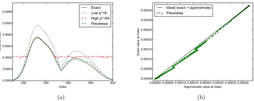
200 250 300 350 400 Index
0.0000 0.0001 0.0002 0.0003 0.0004 0.0005 0.0006
Value at index
Exact Low p*=8 High p*=64 Piecewise
(a)
0.00000 0.00005 0.00010 0.00015 0.00020 0.00025 0.00030 0.00035 Approximate value at index
0.00000 0.00005 0.00010 0.00015 0.00020 0.00025 0.00030 0.00035
Exact value at index
Ideal( exact = approximate) Piecewise
(b)
Figure 2: The accuracy of numerical fast max-convolution methods. (a)Different
approx-imations for a sample max-convolution problem. The low-p∗ method is underflow-stable, but overestimates the result. The high-p∗ method is accurate when underflow-stable, but experiences underflow at many indices. The piecewise method stitches together ap-proximations from different p∗ to maintain underflow-stability. (b) Exact vs. piecewise approximation at various indices of the same problem. A clear banding pattern is observed with one tight, elliptical cluster for each contour. The slope of the clusters deviates more for the contours using lowerp∗ values.
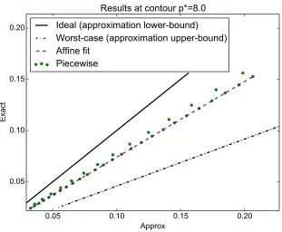
3.3 Improved Affine Piecewise Method
Figure 2b depicts a scatter plot of the exact result vs. the piecewise approximation at every index (using the same problem from Figure 2a). It shows a clear banding pattern: the exact and approximate results are clearly correlated, but each contour (i.e., each collection of indices that use a specificp∗) has a different average slope between the exact and approximate values, with higherp∗
contours showing a generally larger slope and smallerp∗ contours showing greater spread and lower
slopes. This intuitively makes sense, because the bounds on ku(m)k
∞ ∈ [ku(m)kp∗k −1 p∗
m ,ku(m)kp∗]
derived above constrain the scatter plot points inside a quadrilateral envelope (Figure 3).
The correlations within each contour can be exploited to correct biases that emerge for smaller
p∗ values. In order to do this, ku(m)k∞ must be computed for at least two points m1 and m2
within the contour, so that a mappingku(m)kp∗≈f(ku(m)kp∗) =aku(m)kp∗+bcan be constructed.
Fortunately, a single ku(m)k∞ can be computed exactly in O(k) (by actually computing a single u(m) and computing its max, which is equivalent to computing a single index result via the naive
quadratic method). As long as the exact value ku(m)k∞ is computed for only a small number of
indices, the order of the runtime will not change (each contour already costsO(klog2(k)), so adding a small number ofO(k) steps for each contour will not change the asymptotic runtime).
If the two indices chosen are
mmin= argmin
m∈contour(p∗)
ku(m)kp∗
and
mmax= argmax
m∈contour(p∗)
ku(m)kp∗,
0.05
0.10
0.15
0.20
Approx
0.05
0.10
0.15
0.20
Exact
Results at contour p*=8.0
Ideal (approximation lower-bound)
Worst-case (approximation upper-bound)
Affine fit
Piecewise
Figure 3: A single contour from the piecewise approximation. The cluster of points (one
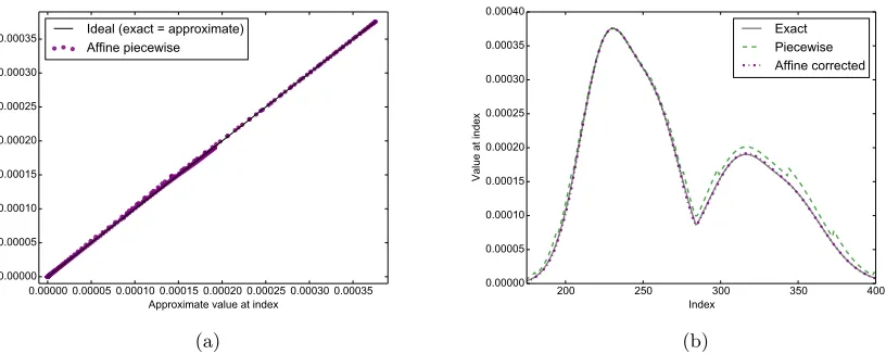
0.00000 0.00005 0.00010 0.00015 0.00020 0.00025 0.00030 0.00035 Approximate value at index
0.00000 0.00005 0.00010 0.00015 0.00020 0.00025 0.00030 0.00035
Exact value at index
Ideal (exact = approximate) Affine piecewise
(a)
200 250 300 350 400 Index
0.00000 0.00005 0.00010 0.00015 0.00020 0.00025 0.00030 0.00035 0.00040
Value at index
Exact Piecewise Affine corrected
(b)
Figure 4: Piecewise method with affine contour fitting. The approximate values at each index of the max-convolution problem are almost identical to the exact result at the same index.
Algorithm 3 Improved affine piecewise numerical max-convolution, a numerical method to estimate the max-convolution nonnegative vectors (further revised to reduce numerical error). This procedure uses ap∗ close to the largest possible stable value at each result index. The return value is a numerical estimate of the max-convolutionL∗maxR. The runtime is inO(klog2(k) log2(p∗max)).
1: procedurenumericalMaxConvolvePiecewiseAffine(L,R,p∗max)
2: `max←argmax`L[`]
3: rmax←argmaxrR[r]
4: L0← L L[`max]
5: R0← R
R[rmax] .Scale to a proportional problem onL
0
, R0
6: allP Star←[20,21, . . . ,2
log2(p∗max)
]
7: fori∈ {0,1, . . . len(allP Star)}do
8: resF orAllP Star[i]←fftNonnegMaxConvolveGivenPStar(L0,R0,allP Star[i])
9: end for
10: form∈ {0,1, . . . len(L) +len(R)−1}do
11: maxStableP StarIndex[m]←max{i: (resF orAllP Star[i][m])allPStar[i]≥τ)}
12: end for
13: result←affineCorrect(resF orAllP Star, maxStableP StarIndex)
14: returnL[`max]×R[rmax]×result .Undo previous scaling
15: end procedure
f(ku(m)kp∗) =λmku(mmax)k∞+ (1−λm)ku(mmin)k∞ λm=
ku(m)k
p∗− ku(mmin)kp∗ ku(mmax)kp∗− ku(mmin)kp∗
∈[0,1]
Thus, by computingku(mmin)k
∞andku(mmax)k∞ (each inO(k) steps), we can compute an affine
functionf to correct contour-specific trends (Algorithm 3).
3.3.1 Error Analysis of Improved Affine Piecewise Method
Algorithm 4 Subroutine for correcting errors in a contour, with an affine transformation based on exact boundary points. It needs the results of the evaluation of the different p-norms as well as the (index of the) maximum stable values ofp∗ at every index.
1: procedureaffineCorrect(resF orAllP Star,maxStableP StarIndex)
2: ∀i, slope[i]←1
3: ∀i, bias[i]←0
4: usedP Star←set(maxStableP StarIndex)
5: fori∈usedP Stardo
6: contour← {m:maxStableP StarIndex[m] =i}
7: mM in←argminm∈contourresF orAllP Star[i][m]
8: mM ax←argmaxm∈contourresF orAllP Star[i][m]
9: xM in←resF orAllP Star[i][mM in]
10: xM ax←resF orAllP Star[i][mM ax]
11: yM in←maxConvolutionAtIndex(mM in)
12: yM ax←maxConvolutionAtIndex(mM ax)
13: if xM ax > xM inthen
14: slope[i]← yM ax−yM in xM ax−xM in
15: bias[i]←yM in−slope[i]×xM in
16: else
17: slope[i]←yM ax xM ax
18: end if
19: end for
20: form∈ {0,1, . . . len(L) +len(R)−1}do
21: i←maxStableP StarIndex[m]
22: result[m]←resF orAllP Star[i][m]×slope[i] +bias[i]
23: end for
24: returnresult
are now interpolating. If the two points used to determine the parameters of the affine function were not chosen in this manner to fit the affine function, then it would be possible to choose two points with very close x-values (i.e., similar approximate values) and disparate y-values (i.e., different exact values), and extrapolating to other points could propagate a large slope over a large distance; using the extreme points forces the affine function to be a convex combination of the extrema, thereby avoiding this problem.
f(ku(m)kp∗) =λmku(mmax)k∞+ (1−λm)ku(mmin)k∞ ∈
"
λm
ku(mmax)k
p∗
k 1 p∗
mmax
+ (1−λm)
ku(mmin)k
p∗
k 1 p∗
mmin ,
λmku(mmax)kp∗+ (1−λm)ku(mmin)kp∗
i
⊆
λm
ku(mmax)k
p∗
kp1∗
+ (1−λm)
ku(mmin)k
p∗
kp1∗ ,
λmku(mmax)kp∗+ (1−λm)ku(mmin)kp∗
i
=hk−1p∗
λmku(mmax)kp∗+ (1−λm)ku(mmin)kp∗
,
λmku(mmax)kp∗+ (1−λm)ku(mmin)kp∗
i
= hk−1p∗ku(m)kp∗,ku(m)kp∗
i
The worst-case absolute error of the scaled problem onL0, R0 can be defined as
max m | f(ku
(m)
kp∗)− ku(m)k∞ |.
Because the function f(ku(m)k
p∗)− ku(m)k∞ is affine, it’s derivative can never be zero, and thus
Lagrangian theory states that the maximum must occur at a boundary point. Therefore, the worst-case absolute error is
≤ max{ku(m)kp∗− ku(m)k∞,ku(m)k∞− ku(m)kp∗k −1 p∗}
= ku(m)kp∗− ku(m)k∞,
which is identical to the worst-case error bound before applying the affine transformationf. Thus applying the affine transformation can dramatically improve error, but will not make it worse than the original worst-case.
3.4 An Improved Approximation of the Chebyshev Norm
In order to improve the error of the piecewise numerical method, we consider the worst-case, when u(m)
ku(m)k∞ = (1,1, . . .1). In this case, computing any two norms of u
(m) (at p∗
1 and p∗2) would be
sufficient to solve exactly forku(m)k
∞, because
ku(m)kp∗1
p∗
1 ∝ ku (m)kp∗1
∞
ku(m)kp∗2
p∗
2 ∝ ku (m)
kp∗2 ∞,
Thus we see that although thep∗-norm approximation of the Chebyshev norm is a good approx-imation, the curve of the norms (at various different p∗) values holds far more information than a simple point estimate would. Therefore, we derive an improved algorithm by proceeding as follows: First, we note that, rather than computing the p∗-norm of a vectoru(m) by summing all elements ofu(m)taken to the powerp∗, it is possible to equivalently sum over only the unique values ofu(m)
(here denoted inβ1, β2, . . .) taken to thep∗ where each term in the sum is weighted by the number
of occurrences of each (denotedh1, h2, . . ., respectively). For this reason, we can then use a sequence
of norms to compute a (potentially smaller) collection of approximate unique values α1, α2, . . . αr, where once again, thep∗-norm is equal to the sum over those unique values to the p∗, where each term in the sum is weighted by numbers of occurrencesn1, n2, . . . nr. Therefore, given 2r different norms of u(m), it is possible to project and estimate r unique α
i values. The maximum of those
α1, α2, . . . αr values, (the α1, α2, . . . αr values can be thought of as projections of the true unique valuesβ1, β2, . . .) can then be used as an estimate of the true maximum element inu(m), which we
will now demonstrate.
Specifically, wherekm is the length ofu(m) and where there are em≤kmunique values (βi) in
u(m), we can model the norms perfectly with
ku(m)kpp∗∗=
em
X
i
hiβp
∗
i
wherehiis an integer that indicates the number of timesβioccurs inu(m)(and wherePihi=km=
len(u(m))). This multi-set view of the vectoru(m) can be used to project it down to a dimensionr:
αp1∗ αp2∗ αpr∗
α21p∗ α22p∗ · · · α2p∗ r
α31p∗ α32p∗ α3rp∗ ..
. ... ...
α`p1∗ α`p2∗ α`p∗ r · n1 n2 n3 .. . nr =
ku(m)kp∗ p∗ ku(m)k2p∗
2p∗ ku(m)k3p∗
3p∗
.. .
ku(m)k`p∗ `p∗ .
By solving the above system of equations for all αi, the maximum ˆα = maxiαi can be used to approximate the true maximum maxiβi=ku(m)k∞. This projection can be thought of as querying distinct moments of the distribution pmfU(m) that corresponds to some unknown vectoru(m), and
then assembling the moments into a model in order to predict the unknown maximum value in
u(m). Of course, when r, the number of terms in our model, is sufficiently large, then computingr
norms ofu(m) will result in an exact result, but it could result in O(k
m) execution time, meaning that our numerical max-convolution algorithm becomes quadratic; therefore, we must consider that a small number of distinct moments are queried in order to estimate the maximum value in u(m).
Regardless, the system of equations above is quite difficult to solve directly via elimination for even very small values of r, because the symbolic expressions become quite large and because symbolic polynomial roots cannot be reliably computed when the degree of the polynomial is >5. Even in cases when it can be solved directly, it will be far too inefficient.
For this reason, we solve for the αi values using an exact, alternative approach: If we define a polynomialγ(x) =x−αp1∗ x−α2p∗· · · x−αp∗
r
, then x∈ {αp1∗, αp2∗, . . . αp∗
γ0 γ1 γ2 · · · γr ·
αp1∗ αp2∗ αp∗ r
α21p∗ α22p∗ · · · α2p∗ r
α31p∗ α32p∗ α3p∗ r ..
. ... ...
α1`p∗ α`p2∗ α`p∗ r · n1 n2 n3 .. . nr = h
α1p∗γ(αp1∗) αp2∗γ(α2p∗) αp3∗γ(αp3∗) · · · αp∗ r γ(αp
∗ r ) i · n1 n2 n3 .. . nr =
0 0 0 · · · 0
· n1 n2 n3 .. . nr
= 0,
which indicates that
γ0 γ1 γ2 · · · γr ·
ku(m)kp∗ p∗ ku(m)k2p∗
2p∗ ku(m)k3p∗
3p∗
.. .
ku(m)k`p∗ `p∗
= 0.
Furthermore,γ(x) = 0, x6= 0⇔xiγ(x) = 0, i∈N; therefore we can write
γ0 γ1 γ2 · · · γr 0 0 · · · 0 0 γ0 γ1 γ2 · · · γr 0 · · · 0 0 0 γ0 γ1 γ2 · · · γr · · · 0
.. .
0 0 · · · 0 γ0 γ1 γ2 · · · γr ·
ku(m)kp∗ p∗ ku(m)k2p∗
2p∗ ku(m)k3p∗ 3p∗
.. .
ku(m)k`p`p∗∗
=
ku(m)kpp∗∗ ku(m)k2p ∗
2p∗ ku(m)k 3p∗
3p∗ · · · ku(m)k (r+1)p∗
(r+1)p∗ ku(m)k2p∗
2p∗ ku(m)k 3p∗
3p∗ ku(m)k 4p∗
4p∗ · · · ku(m)k (r+2)p∗
(r+2)p∗ ku(m)k33pp∗∗ ku(m)k4p
∗
4p∗ ku(m)k5p ∗
5p∗ · · · ku(m)k (r+3)p∗
(r+3)p∗
..
. ... ... ...
ku(m)k(`−r)p∗
(`−r)p∗ ku(m)k
(`−r+1)p∗
(`−r+1)p∗ ku(m)k
(`−r+2)p∗
(`−r+2)p∗ · · · ku(m)k
`p∗ `p∗ · γ0 γ1 γ2 .. . γr
= 0.
Therefore, γ0 γ1 γ2 .. . γr ∈null
ku(m)kp∗
p∗ ku(m)k 2p∗
2p∗ ku(m)k 3p∗
3p∗ · · · ku(m)k (r+1)p∗
(r+1)p∗ ku(m)k2p∗
2p∗ ku(m)k 3p∗
3p∗ ku(m)k 4p∗
4p∗ · · · ku(m)k (r+2)p∗
(r+2)p∗ ku(m)k3p∗
3p∗ ku(m)k 4p∗
4p∗ ku(m)k 5p∗
5p∗ · · · ku(m)k (r+3)p∗
(r+3)p∗
..
. ... ... ...
ku(m)k((``−−rr))pp∗∗ ku
(m)k(`−r+1)p∗
(`−r+1)p∗ ku
(m)k(`−r+2)p∗
(`−r+2)p∗ · · · ku (m)k`p∗
Because the columns of
αp1∗ αp2∗ αpr∗
α21p∗ α22p∗ · · · α2p∗ r
α31p∗ α32p∗ α3rp∗ ..
. ... ...
α`p1∗ α`p2∗ α`p∗ r
must be linearly independent when α1, α2, . . . are distinct (which is the case by the definition of
our multiset formulation of the norm), then r = 2` will determine a unique solution; thus the null space above is computed from a matrix with r+ 1 columns and r rows, yielding a single vector for (γ0, γ1, . . . γr). This vector can then be used to compute the roots of the polynomial
γ0+γ1x+γ2x2+· · ·+γrxr, which will determine the values {α p∗
1 , α
p∗
2 , . . . αp ∗
r }, which can each be taken to the p1∗ power to compute {α1, α2, . . . , αr}; the largest of those αi values is used as the estimate of the maximum element inu(m). When u(m) contains at leastrdistinct values (i.e., em≥r), then the problem will be well-defined; thus, if the roots of the null space spanning vector are not well-defined, then a smallerrcan be used (and should be able to compute an exact estimate of the maximum, sinceu(m)can be projected exactly whenris the precise number of unique elements
found inu(m)).
To summarize, the null space projection method is performed as follows: First, standard FFT-based convolution is used for each p∗ to compute the different norms at every index m. Then those norms are used to populate and compute the null space of a matrix. Finally the roots of the polynomial whose coefficients are given by the null space vector are computed to estimate the differentα1, α2, . . .. Note that this projection method is valid for any sequence of norms with even
spacing: ku(m)kp ∗ 0+p
∗
p0+p∗,ku
(m)kp0+2p∗
p0+2p∗,ku
(m)kp0+3p∗
p0+3p∗, . . .ku
(m)kp0+`p∗
p0+`p∗.
The null space projection method can therefore be computed for an arbitraryr(i.e., it can be used to project to an arbitrary number of unique elements in u(m)) by using linear algebra to compute
the null space and to compute the roots of the polynomial (for instance, using the numpy.roots
command in Python). For greater efficiency, settingrto a small constant allows us to precompute closed-form solutions of both the null space and the polynomial roots. For instance, using r = 2 (which is equivalent to projecting each vectoru(m)to two unique values) results in a
R3×2null space
computation and computing roots of a quadratic polynomial, both of which can be done in closed form Algorithm 5. Details of this r = 2 case can be found in Appendix 5. In this case, it is possible to construct a series of powers of two with interleaved points, which guarantees that 4 evenly spacedp∗ values exist (when the highest numerically stable p∗ is higher than 2), meaning that the number of FFT calls is only 2×what would be used by the original piecewise method (rather than 4×the calls, which would be necessary if 4 evenly spaced points were placed at each considered p∗
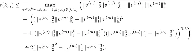
in a naive scheme). From algebraic and empirical evidence, we conjecture that the relative error of thisr= 2 null space projection is bounded above by 1−0.7p4∗, wherep∗ is the highest numerically
stablep∗ value.
This relative error is superior to the worst-case relative error when using a singlep∗-norm estimate
of the maximum. The relative error using the null space projection decreases rapidly as p∗ is
increased, meaning that the same procedure can be used to achieve an absolute error bound:
ˆ
α− ku(m)k∞< τ 1 2p∗
1−0.7p4∗
,
which achieves a unique maximum at
p∗mode= 1.4267∗log(τ)−4.07094 (log(τ)−2.8534)log(1−2.8534
log(τ))
Algorithm 5 Piecewise numerical max-convolution with projection, a numerical method to estimate the max-convolution of two PMFs or nonnegative vectors. This method uses a nullspace projection to achieve a closer estimate of the true maximum. Depending on the number of stable estimates, linear or quadratic projection is used. The parameters are two nonnegative vectors L0
andR0(both scaled so that they have maximal element 1). The return value is a numerical estimate of the max-convolutionL0 ∗max R0.
1: procedurenumericalMaxConvolvePiecewiseProjectionAffine(L0,R0,p∗)
2: `max←argmax`L[`]
3: rmax←argmaxrR[r]
4: L0← L L[`max]
5: R0← R
R[rmax] .Scale to a proportional problem onL
0
, R0
6: allP Star←[2−1,20,21, . . . ,2 + 2
log2(p∗max)
]
7: forh∈ {0,1, . . . len(allP Star)}do
8: allP StarInterleaved[2i]←allP Star[i]
9: allP StarInterleaved[2i+ 1]←0.5×(allP Star[i] +allP Star[i+ 1])
10: end for
11: fori∈ {0,1, . . . len(allP Star)}do
12: resF orAllP Star[i]←fftNonnegMaxConvolveGivenPStar(L0,R0,allP StarInterleaved[i])
13: end for
14: form∈ {0,1, . . . len(L) +len(R)−1}do
15: maxStableP StarIndex[m]←max{i: (resF orAllP Star[i][m])allPStarInterleaved[i]≥τ)}
16: end for
17: foro∈ {0,1, . . . len(maxStableP StarIndex)}do
18: maxStableP StarIndex[o]−=maxStableP StarIndex[o]%2 .Restrict to powers of 2
19: end for
20: forp∈ {0,1, . . . len(maxStableP StarIndex)}do
21: maxP ←allP StarInterleaved[maxStableP StarIndex[p]]
22: spacing←0.25∗maxP
23: est4←resF orAllP Star[maxStableP StarIndex[p]]
24: est3←resF orAllP Star[maxStableP StarIndex[p]−1]
25: if maxStableP StarIndex[p]<5then .Need 5p∗in sequence to get 4 evenly spaced
26: resF orAllP Star[p]←maxLin(est3, est4)
27: else
28: est2←resF orAllP Star[maxStableP StarIndex[p]−2]
29: est1←resF orAllP Star[maxStableP StarIndex[p]−4] .Index - 4 is the next evenly spaced point
30: resF orAllP Star[p]←maxQuad(est1, est2, est3, est4, spacing)
31: end if
32: end for
33: result←affineCorrect(resF orAllP Star, maxStableP StarIndex)
34: returnL[`max]×R[rmax]×result .Undo previous scaling
As before, the worst-case absolute error of the unscaled problem will be found by simply scaling the absolute error atp∗mode:
max
` L[`] maxr R[r]τ
1 2p∗mode
1−0.7
4 p∗mode
.
Becausep∗mode(the value ofp∗producing the worst-case absolute error) for the null space projection method it is invariant to the length of the list k (enabling us to compute a numeric value), and because its numeric value is so small, even a fairly small choice ofp∗maxwill suffice (nowp∗max∈O(1) rather than inO(log(k)) as it was with the original piecewise method).
The one caveat of this worst-case absolute error bound is that it presumes at least four evenly spaced, stable p∗ can be found (which may not be the case by choosing p∗ from the sequence 2i in cases when ku(m)k∞ ≈ 0); however, assuming standard fast convolution can be performed (a reasonable assumption given it is one of the essential numeric algorithms), then four evenly spaced
p∗values could be chosen very close to 1; therefore, these values ofp∗could be added to the sequence so that the algorithm is slightly slower, but essentially always yield this worst-case absolute error bound.
In practice, we can demonstrate that the null space projection method is very accurate. First we show the impact of using the quadratic (i.e., r= 2) projection method on unscaled singleu(m)
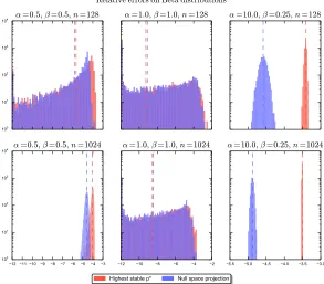
vectors. The projection method was tested on vectors of different lengths drawn from different types of Beta distributions and are compared with the results of the p-norms with the highest stablep
(Figure 5). The relative errors between the original piecewise method and the null space projection method are compared using a max-convolution on two randomly created input PMFs of lengths 1024 (Figure 6). Note that the null space projection can also be paired with affine scaling on the back end, just as the original piecewise method can be. In practice, the null space projection increases the accuracy demonstrably on a variety of different problems, although the original piecewise method also performs well.
Although the worst-case runtime of the null space projection method is roughly 2×that of the original piecewise method, the error bound no longer depends on the length of the resultk. Thus, for a given relative error bound on the top contour (i.e., the equivalent of the derivation ofp∗max in the original piecewise algorithm), the value ofp∗maxis fixed and no longer∈O(log(k)). For example, achieving a 0.5% relative error in the top contour would require
1−0.7p∗max4 ≤0.005→p∗ max≥4
log(0.7)
log(0.995) ≈284.62,
meaning that choosingp∗max = 512 would achieve a very high accuracy, but while only performing
2×9 FFTs. For very large vectors, this will not be substantially more expensive than the original piecewise algorithm, which uses a higher value of p∗
max (in this case, p∗max = log1.005(k), which
continues to grow as k does) to keep the error lower in practice. As a result, the runtime of the null space projection approximation is∈O(klog(k)) rather thanO(klog(k) log(log(k))), despite the similar runtime in practice to the original piecewise method (the null space projection method uses 2×as many FFTs performed perp∗ value, but requires slightly fewerp∗ values).
3.5 Practical Runtime Comparison
100 101 102 103
104
α
=0.
5, β
=0.
5, n
=128α
=1.
0, β
=1.
0, n
=128α
=10.
0, β
=0.
25, n
=12812 11 10 9 8 7 6 5 4 3 100
101 102 103
104
α
=0.
5, β
=0.
5, n
=102412 10 8 6 4 2
α
=1.
0, β
=1.
0, n
=10245.5 5.0 4.5 4.0 3.5 3.0
α
=10.
0, β
=0.
25, n
=1024Relative errors on Beta distributions
Highest stable p* Null space projection
Figure 5: Relative errors on random vectors with and without null space projection. For
0 500 1000 1500 2000 2500 3000 3500 4000 4500 0.0
0.1 0.2 0.3 0.4 0.5 0.6 0.7
Highest stable p*
Null space projection
0.0 0.2 0.4 0.6 0.8 1.0 1.2 1e 6
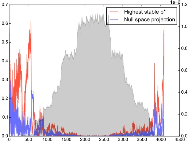
Figure 6: Relative errors on large max-convolution with and without null space
projec-tion. Max-convolution between two randomly generated vectors (both uniform vectors convolved with narrow Gaussians with uniform noise added afterward), performed with the highest stable p∗-norm (using the heuristic choice of p∗max for problems of this size) and with null space projection (usingp∗max= 64). The left y-axis shows the relative error
at indexm. Associated with that, you can see the red and blue curve depicting the errors from the two different methods: Red describes the max-norm estimation using only the highest stablep∗while purple was generated using quadratic projection at the four highest
k 26 27 28 29 210 211 212
Naive 0.0142 0.0530 0.192 0.767 3.03 12.1 48.2
Naive (vectorized) 0.0175 0.0381 0.0908 0.251 0.790 2.75 10.1
FILL1 (Bussieck et al., 1994) 0.0866 1.09 7.21 19.4 457 — —
Max. stablep∗, affine corrected 0.0277 0.0353 0.0533 0.0848 0.149 0.274 0.537
Projection, affine corrected 0.0236 0.0307 0.0467 0.0760 0.137 0.258 0.520
Table 1: Runtimes of different methods for max-convolution on uniform vectors of length
k. The runtimes were gathered using thetimeitpackage in Python. They include all pre-processing steps necessary for the algorithm (e.g., sorting prior to the FILL1 approach). The values are total runtimes (in seconds) to run 5 repetitions on different, randomly gen-erated vectors. FILL1 was not run on larger problems, because it ran substantially longer than the non-vectorized naive approach. On the two approximation methods presented in this manuscript, the highest stablep∗-norm approximation was run with the heuristically chosen p∗
max for problems of the appropriate size and the null space projection was run
withp∗max= 64.
pseudocode in their manuscript. From their variants of proposed methods, FILL1 was chosen because of its use in their corresponding benchmark and its recommendation by the authors for having a lower runtime constant in practice compared to other methods they proposed. The method is based on sorting the input vectors and traversing the (implicitly) resulting partially ordered matrix of products in a way that not all entries need to be evaluated, while only keeping track of the so-called cover of maximal elements. FILL1 already includes some more sophisticated checks to keep the cover small and thereby reducing the overhead per iteration. Unfortunately, although we observed that the FILL1 method requires betweenO(nlog(n)) andO(n2) iterations in practice, this per-iteration
overhead results in a worst-case cost of log(n) per iteration, yielding an overall runtime in practice between O(nlog(n) log(n)) and O(n2log(n)). As the authors state, this overhead is due to the
expense of storing the cover, which can be implemented e.g., using a binary heap (recommended by the authors and used in this reimplementation). Additionally, due to the fairly sophisticated datastructures needed for this algorithm it had a higher runtime constant than the other methods presented here, and furthermore we saw no means to vectorize it to improve the efficiency. For this reason, it is not truly fair to compare the raw runtimes to the other vectorized algorithms (and it is not likely that this Python reimplementation is as efficient as the original version, which Bussieck et al., 1994 implemented in ANSI-C); however, comparing a non-vectorized implementation of the naiveO(n2) approach with its vectorized counterpart gives an estimated≈5×speedup from vectorization, suggesting that it is not substantially faster than the naive approach on these problems (it should be noted that whereas the methods presented here have tight runtime bounds but produce approximate results, the FILL1 algorithm is exact, but its runtime depends on the data processed). During investigation of these runtimes, we found that on the given problems, the proposed average case of O(nlog(n)) iterations was rarely reached. A reason might be an unrecognized violation of the assumptions of the theory behind this theoretical average runtime in how the input vectors were generated.
3.6 Demonstration on Hidden Markov Model With Toeplitz Transition Matrix
One example that profits from fast max-convolution of non-negative vectors is computing the Viterbi path using a hidden Markov model (HMM) (i.e., themaximum a posterioristates) with an additive transition function satisfying Pr(Xi+1=a|Xi =b)∝δ(a−b) for some arbitrary functionδ(δ can be represented as a table, because we are considering all possible discrete functions). This additivity constraint is equivalent to the transition matrix being a “Toeplitz matrix”: the transition matrix
Ta,b = Pr(Xi+1 = a|Xi =b) is a Toeplitz matrix when all cells diagonal from each other (to the upper left and lower right) have identical values (i.e., ∀a,∀b, Ta,b = Ta+1,b+1). Because of the
Markov property of the chain, we only need to max-marginalize out the latent variable at time i
to compute the distribution for the next latent variable Xi+1 and all observed values of the data
variablesD0. . . Di+1. This procedure, called the Viterbi algorithm, is continued inductively:
max x0,x1,...xi−1
Pr(D0, D1, . . . Di−1, X0=x0, X1=x1, . . . , Xi=xi) =
max xi−1
max x0,x1,...xi−2
Pr(D0, D1, . . . Di−2, X0=x0, X1=x1, . . . , Xi−1=xi−1)
Pr(Di−1|Xi−1=xi−1) Pr(Xi=xi|Xi−1=xi−1)
and continuing by exploiting the self-similarity on a smaller problem to proceed inductively with variable f romLef t, revealing a max-convolution (for this specialized HMM with additive transi-tions):
max x0,x1,...xi−1
Pr(D0, D1, . . . Di−1, X0=x0, X1=x1, . . . , Xi=xi) = max
xi−1
f romLef t[i−1] Pr(Di−1|Xi−1=xi−1)δ[xi−xi−1] =
(f romLef t[i−1]likelihood[Di−1]) ∗max δ[xi−xi−1].
After computing this left-to-right pass (which consisted of n−1 max-convolutions and vec-tor multiplications), we can find the maximum a posteriori configuration of the latent variables
X0, . . . Xn−1 = x∗0, . . . x∗n−1 backtracking right-to-left, which can be done by finding the variable
value xi that maximizes f romLef t[i][xi]×δ[x∗i+1−xi] (thus defining x∗i and enabling induction on the right-to-left pass). The right-to-left pass thus requires O(nk) steps (Algorithm 6). Note that the full max-marginal distributions on each latent variable Xi can be computed via a small modification, which would perform a more complex right-to-left pass that is nearly identical to the left-to-right pass, but which performs subtraction instead of addition (i.e., by reversing the vector representation of the PMF of the subtracted argument before it is max-convolved; Serang, 2014).
Algorithm 6 Viterbi for models with additive transitions, which accepts the lengthkvector
prior, a list of n binned observations data, a a×k matrix of likelihoods (where a is the number of bins used to discretize the data) likelihoods, and a length 2k−1 vector δ that describes the transition probabilities. The algorithm returns a Viterbi path of length n, where each element in the path is a valid state∈ {0,1, . . . k−1}.
1: procedureViterbiForAdditiveTransitions(prior, data, likelihood, δ)
2: f romLef t[0]←prior
3: fori= 0 ton−2do
4: f romLef t[i]←f romLef t[i]×likelihood[data[i]]
5: f romLef t[i+ 1]←f romLef t[i]∗maxδ
6: end for
7: f romLef t[n]←f romLef t[n]×likelihood[data[n]]
8:
9: path[n−1]←argmaxjf romLef t[n−1][j]
10: fori=n−2 to 0do
11: maxP rodP osterior← −1
12: argmaxP rodP osterior← −1
13: forl=kto 1do
14: currP rodP osterior←f romLef t[i]×δ[l−path[i+ 1]]
15: if currP rodP osterior > maxP rodP osteriorthen
16: maxP rodP osterior←currP rodP osterior
17: argmaxP rodP osterior←l
18: end if
19: end for
20: path[i]←argmaxP rodP osterior
21: end for
22: returnpath
short amount of time) and current stock market prices (the observed data). We discretized random variables for the observed data (S&P 500, adjusted closing prices ; retrieved from YAHOO! his-torical stock prices: http://data.bls.gov/cgi-bin/surveymost?blsseriesCUUR0000SA0), and ”latent” variables (unemployment insurance claims, seasonally adjusted, were retrieved from the U.S. Department of Labor: https://www.oui.doleta.gov/unemploy/claims.asp). Stock prices were additionally inflation adjusted by (i.e., divided by) the consumer price index (CPI) (retrieved from the U.S. Bureau of Labor Statistics: https://finance.yahoo.com/q?s=^GSPC). The inter-section of both ”latent” and observed data was available weekly from week 4 in 1967 to week 52 in 2014, resulting in 2500 data points for each type of variable.
To investigate the influence of overfitting, we partition the data in two parts, before June 2005 and after June 2005, so that we are effectively training on 2000×1002500 = 80% of the data points, and then demonstrate the Viterbi path on the entirety of the data (both the 80% training data and the 20% of the data withheld from empirical parameter estimation). Unemployment insurance claims were discretized into 512 and stock prices were discretized into 128 bins. Simple empirical models of the prior distribution for unemployment, the likelihood of unemployment given stock prices, and the transition probability of unemployment were built as follows: The initial or prior distribution for unemployment claims ati= 0 was calculated by marginalizing the time series of training data for the claims (i.e., counting the number of times any particular unemployment value was reached over all possible bins). Our transition function (the conditional probability Pr(Xi+1|Xi)) similarly counts the number of times each possible change Xi+1−Xi∈ {−511,−510, . . .511}occurred over all available time points. Interestingly, the resulting transition distribution roughly resembles a Gaussian (but is not an exact Gaussian). This underscores a great quality of working with discrete distributions: while continuous distributions may have closed-forms for max-convolution (which can be computed quickly), discrete distributions have the distinct advantage that they can accurately approximate any smooth distribution. Lastly, the likelihoods of observing a stock price given the unemployment at the same time were trained using an empirical joint distribution (essentially a heatmap), which is displayed inFigure 7.
We compute the Viterbi path two times: First we use naive, exact max-convolution, which requires a total of O(nk2) steps. Second, we use fast numerical max-convolution, which requires O(n klog(k) log(log(k)) steps. Despite the simplicity of the model, the exact Viterbi path (computed via exact max-convolution) is highly informative for predicting the value of unemployment, even for the 20% of the data that were not used to estimate the empirical prior, likelihood, and transition distributions. Also, the numerical convolution method is nearly identical to the exact max-convolution method at every index (Figure 8). Even with a fairly rough discretization (i.e., k= 512), the fast numerical method (via the original, simpler piecewise algorithm with p∗max = 8192)
used 141.4 seconds compared to the 292.3 seconds required by the naive approach. The higher-precision projection algorithm (which uses a smallerp∗
max, but calls FFT twice for each power of two p∗) computes nearly identical result usingp∗max= 64 for this problem in 136.6 seconds. The speedup of both fast numerical algorithms relative to the naive quadratic max-convolution algorithm will increase dramatically askis increased.
4. Discussion
Both piecewise numerical max-convolution methods are highly accurate in practice and achieve a substantial speedup over both the naive approach and the approach proposed by Bussieck et al. (1994). This is particularly true for large problems: For the original piecewise method presented here, the log2(log1+τ1
4(k)) multiplier may never be small, but it grows so slowly with k that it
0
500
1000
1500
2000
2500
Week
0
100
200
300
400
500
600
700
800
New unemployment claims (binned)
True unemployment values
Exact Viterbi estimate
Numerical Viterbi estimate
becomes more pronounced as k becomes large. For the second method presented (the null space projection), the runtime for a given relative error bound will be inO(klog2(k)). In practice, both methods have similar runtime on moderate or large problems.
The basic motivation of the first approach described—i.e., the idea of approximating the Cheby-shev norm with the largestp∗-norm that can be computed accurately, and then convolving according to this norm using FFT—also suggests further possible avenues of research. For instance, it may be possible to compute a single FFT (rather than an FFT at each of several contours) on a more precise implementation of complex numbers. Such an implementation of complex values could store not only the real and imaginary components, but also other much smaller real and imaginary components that have been accumulated through + operations, even those which have small enough magnitudes that they are dwarfed by other summands. With such an approach it would be possible to numeri-cally approximate the max-convolution result in the same overall runtime as long as only a bounded “history” of such summands was recorded (i.e., if the top few magnitude summands—whether that be the top 7 or the top log2(log
1+τ14(k))—was stored and operated on). In a similar vein, it would
be interesting to investigate the utility of complex values that use rational numbers (rather than fixed-precision floating point values), which will be highly precise, but will increase in precision (and therefore, computational complexity of each arithmetic operation) as the dynamic range between the smallest and largest nonzero values inLandRincreases (because takingL0 to a large powerp∗
may produce a very small value). Other simpler improvements could include optimizing the error vs. runtime trade-off between the log-base of the contour search: the method currently searches log2(p∗max) contours, but a smaller or larger log-base could be used in order to optimize the trade-off between error and runtime.
It is likely that the best trade-off will occur by performing the fast p∗-norm convolution with a number type that sums values over vast dynamic ranges by appending them in a short (i.e., bounded or constant size) list or tree and sums values within the same dynamic range by querying the list or tree and then summing in at the appropriate magnitude. This is reminiscent of the fast multipole algorithm (Rokhlin, 1985). This would permit the method to use a single large p∗ rather than a piecewise approach, by moving the complexity into operations on a single number rather than by performing multiple FFTs with simple floating-point numbers.
The basic motivation of the second approach described—i.e., using the sequence of p∗-norms (each computed via FFT) to estimate the maximum value—generalizes thep∗-norm fast convolution numerical approach into an interesting theoretical problem in its own right: given an oracle that delivers a small number of norms (the number of norms retrieved must bec∈o(k) to significantly outperform the naive quadratic approach) about each vectoru(m), amalgamate these norms in an
efficient manner to estimate the maximum value in each u(m). This method may be applicable to
other problems, such as databases where the maximum values of some combinatorial operation (in this case themaximum a posterioridistribution of the sum of two random variablesX+Y) is desired but where caching all possible queries and their maxima would be time or space prohibitive. In a manner reminiscent of how we employ FFT, it may be possible to retrieve moments of the result of some combinatoric combination between distributions on the fly, and then use these moments to approximate true maximum (or, in general, other sought quantities describing the distribution of interest).
In practice, the worst-case relative error of our quadratic approximation is quite low. For example, whenp∗= 8 is stable, then the relative error is less than 2.3%, regardless of the lengths of the vectors being max-convolved. In contrast, the worst-case relative error using the original piecewise method would be≤k161 −1, wherekis the length of the max-convolution result (whenn= 1024, the relative
error of the original piecewise method would be≈54%).