A wavelet operational matrix method for solving initial - boundary value problems for fractional partial differential equations

(1)

J. Math. Comput. Sci. 6 (2016), No. 4, 527-539 ISSN: 1927-5307

A WAVELET OPERATIONAL MATRIX METHOD FOR SOLVING INITIAL -BOUNDARY VALUE PROBLEMS FOR FRACTIONAL PARTIAL DIFFERENTIAL

EQUATIONS

RAGHVENDRA SINGH CHANDEL1, AMARDEEP SINGH2AND DEVENDRA CHOUHAN3∗

1_{Department of Mathematics, Govt. Geetanjali Girls College, Bhopal, India} 2_{Department of Mathematics, Govt. MVM College, Bhopal, India}

3∗_{Department of Mathematics, IES, IPS Academy, Indore, India}

Abstract. A fractional partial differential equation (FPDE) is a partial differential equation which involves frac-tional calculus operators. In this paper, the numerical solutions of Initial - Boundary value problems for FPDEs have been approximated using Haar wavelet operational matrix method. The FPDEs are reduced into simple alge-braic equations which can be solved easily by computer aided techniques. The simplicity and effectiveness of the proposed method are illustrated by providing several examples with numerical simulations.

Keywords: Fractional calculus; Fractional partial differential equation; Wavelet analysis; Haar wavelets; Opera-tional matrix.

2010 AMS Subject Classification:42C40, 26A33, 34A08, 34K37.

1. Introduction

In recent years, FPDEs like fractional convection - diffusion equations, Space - time fraction-al advection - dispersion equation etc. have attracted the attentions of many researchers and are

∗_{Corresponding author}

Received October 15, 2015

(2)

becoming increasingly popular due to their applications in various fields of science and engi-neering [10]. The FPDEs have shown to be adequate models for various physical phenomena in areas such as damping laws, diffusion processes etc. Other applications include arterial science, electromagnetism, electro - chemistry, the theory of Ultra - slow processes and finance.

Further it is worthwhile to mention that, a small number of algorithms for the numerical so-lution of FPDEs have been suggested. The need to exploit some efficient and reliable numerical scheme is a problem of fundamental interest. In the literature, small numbers of numerical methods have been proposed for obtaining approximate solutions to FPDEs [1, 4, 5]. The aim of all these studies has been to obtain effective algorithms that are suitable for the digital com-puter. But all these methods have their own advantages, disadvantages and limitations in finding the solution of FPDEs.

Recently, orthogonal wavelet bases are becoming more popular for numerical solutions of partial differential equations. It is because of their excellent properties such as, ability to detect singularities, flexibility to represent a function at different levels of resolution and compact sup-port. In recent years, there has been a growing interest in developing Wavelet based numerical algorithms for solutions of FPDEs.

The Haar wavelet is the simplest example of orthogonal wavelets, compactly supported on the interval [0, 1). Historically Chen and Hsiao [2], first proposed a Haar operational matrix for the integration of Haar function vectors and used it for solving differential equations. Recently, there has been some considerable developments in the application of Wavelet basis to solve differential equations of fractional order [3, 9, 11].

(3)

2. Preliminaries and Basic concepts

2.1 Fractional derivative and integral. The caputo fractional derivative of order α >0, is given as [7],

Dα

t f(t) =

  

 

dm

dtmf(t) α=m∈N 1

Γ(m−α)

Rt a

fm(z)

(t−z)α−m+1dz, 0≤m−1<α <m

Partial Caputo fractional derivative ofy(x,t)∈Cn [0,1]×[0,1]is defined as,

∂α

∂tαy(x,t) =

  

 

In−α

t ∂

n

∂tny(x,t), n−1<α ≤n ∂n

∂tny(x,t), α=n∈N

whereIα

t is the Riemann - Liouville fractional integral given as, I_tαf(t) = 1

Γ(α) Z t

0

(t−z)α−1_f₍_z₎_dz

withI_t0f(t) = f(t).

Fractional differential and integral operators satisfy following basic properties,

(P1) ItαI

β

t f(t) =I

α+β

t f(t)

(P₂) ∂α ∂tαI

β

t y(x,t) =I

β−α

t y(x,t)

(P3) Itα ∂

α

∂tαy(x,t) =y(x,t)−∑

n−1

i=0 t i

i!

∂i ∂tiy(x,t)

t=0

2.2 Haar wavelets and Function approximation. Haar mother wavelet is defined as h(x) = /0(2x)−/0(2x−1)

where /0(x)is a scaling function defined as

/0(x) =

  

 

1, 0≤x<1 0, otherwise Now define

(4)

then for the Hilbert space L₂[0,1], the Haar system {/0,h_j_,_k : 0≤ j,0≤k<2j} forms an or-thonormal basis.

Hence for some fixedJwe may consider the inner product expansion of f ∈L₂[0,1]as,

(1) f(x) =hf,/0i/0(x) +

J−1

∑

j=0

2j−1

∑

k=0

hf,h_j_,_kih_j_,_k(x) =KTH(x)

whereK is 1×2J coefficient vector andH(x)is the Haar function vector given by, H(x) = [/0,h,h₁,0,h1,1,h2,0,− − −,h2,3,− − −,hJ−1,0,− − −,hJ−1,2J₋₁]T

For our convenience let us denote /0=h0, h=h1=h0,0 andhi=hj,kwhere the indexican be obtained from the relationi=2j+k,(i=0,1,2,− − −,m−1 :m=2J). Hence (1) reduced into

f(x) =

m−1

∑

i=0

k_ih_i(x) =KTH(x)

Now on using Haar wavelets, a functiony(x,t)∈L₂[0,1]×[0,1]can be approximated as, y(x,t) =

m−1

∑

i=0

m−1

∑

j=0

c_i_,_jh_i(x)h_j(t) =HT(x)CH(t)

whereCis 2J×2Jcoefficient matrix determined by the inner productc_i_,_j=hh_i(x),hy(x,t),hj(t)ii. Now on using Haar wavelets, the fractional integral of a function f ∈L₂[0,1]can be given as,

Iα

x f(x) =CTIxαH(x) =CT

Iα

x h0(x),Ixαh1(x),− − −,Ixαhm−1(x) T

=CT

hm−1

∑

i=0

A0,ihi(x), m−1

∑

i=0

A1,ihi(x),− − −, m−1

∑

i=0

Am−1,ihi(x)

iT

=CT

           Aα

0,0 Aα0,1 − − − Aα0,m−1

Aα

1,0 Aα1,1 − − − Aα1,m−1

− − − − − −

Aα

m−1,0 Aαm−1,1 − − − Aαm−1,m−1                      

h0(x)

h₁(x)

−

hm−1(x)           

=CTA_αH(x)

(5)

3. Proposed Method

In this section, the properties of Haar wavelets and the operational matrix are used to approx-imate the numerical solutions of Initial - Boundary value problem for FPDEs of the form,

(2) ∂

α

∂tαy(x,t)−a(x) ∂β

∂xβ

y(x,t) +b(x) ∂

γ

∂xγy(x,t) +d(x)y(x,t) = f(x,t)

where 0<α ≤2, 1<β ≤2, 0<γ ≤1 with initial conditions,

(i) y(x,0) =p(x), ∂ ∂ty(x,t)

t=0=q1(x)

OR

(ii) y(x,0) =p(x), y(x,1) =q2(x)

    

   

(3)

and boundary conditions,

(4) y(0,t) = /0(t), y(1,t) =w(t)

Now using the properties of Haar wavelets, we have

(5) ∂

β

∂xβ

y(x,t) =HT(x)CH(t)

On using the property (P3), we have

(6) y(x,t) =Iβ

xHT(x)CH(t) +g(t)x+u(t)

Now on using boundary conditions, we getu(t) = /0(t)and

g(t) =− Z 1

0

(1−z)β−1

Γ(β) H T₍_z₎_dz

!

CH(t) +w(t)−φ(t)

So (6) becomes,

(7) y(x,t) =Iβ

xHT(x)CH(t)−x Z 1

0

(1−z)β−1

Γ(β) H T₍_z₎_dz

!

CH(t) +x w(t)−φ(t)+φ(t)

Now the Haar waveletsψ_j,k;j=0,1,2,− − −,J; 0≤k<2j are supported on dyadic intervals I_j_,_k=

h

k

2j,k+₂j1 i

of[0,1]. Hence Z 1

0

(1−z)β−1

Γ(β) hj,k(z)dz= Z

Ij,k

(1−z)β−1

(6)

Now suppose,I0_j_,−_k =hk

2j, 2k+1

2j+1

i

andI0_j_,+_k =h2k+1

2j+1,

k+1 2j

i

are the left and right halves ofI_j,kSo we have,

Z 1

0

(1−z)β−1

Γ(β) hj,k(z)dz= Z

I0_j_,−_k

(1−z)β−1

Γ(β) hj,k(z)dz− Z

I0_j_,+_k

(1−z)β−1

Γ(β) hj,k(z)dz

Now

uβ_/0 =

Z 1

0

(1−z)β−1

Γ(β) φ(z)dz= 1

Γ(β+1) and

uβ_j_,_k=

Z 1

0

(1−z)β−1

Γ(β) hj,k(z)dz=2 1− 2k+1

2j+1 !β

− 1− k 2j

!β

− 1−k+1 2j

!β

So we have, Z 1

0

(1−z)β−1

Γ(β)

H(z)dz=huβ_/0,u₀β_,₀,uβ₁_,₀,uβ₁_,₁,uβ₂_,₀,− − −,uβ₂_,₃,− − −,uβ_j−₁_,₀,− − −,uβ j−1,2j₋₁

iT

=u₀,u₁,− − −,u_m−₁T

Now suppose, ν :[0,1] →_R is a continuous function. At collocation points xi = ₂2Ji+₊1₁,i=

0,1,− − −,m−1 define a matrixB_β_,_υ as given in [8],

B_β_,_υ =

             

ν(x0)u0 ν(x1)u0 − − − ν(xm−1)u0

ν(x0)u1 ν(x1)u1 − − − ν(xm−1)u1

− − − − − −

ν(x0)um−1 ν(x1)um−1 − − − ν(xm−1)um−1              

Hence by (7),

(8) y(x,t) =HT(x)AT

βCH(t)−B

T

β,νCH(t) +x w(t)−φ(t)

+φ(t)

whereυ(x) =xandA_β is the Haar wavelet operational matrix of fractional integration of order β >0. Now on applying Caputo operator ∂γ

(7)

and property (P2), we have ∂γ

∂xγy(x,t) =I

β−γ

x HT(x)CH(t)− Z 1

0

x1−γ₍₁₋_z₎β−1

Γ(β)Γ(2−γ) H T₍_z₎_dz

!

CH(t)

+x

1−γ _w₍_t₎₋_φ₍_t₎

Γ(2−γ) (9)

Now on substituting (5), (7) and (9) in (2), we have ∂α

∂tαy(x,t) =a(x)H

T₍_x₎_CH₍_t₎₋_b₍_x₎_HT₍_x₎_AT

β−γCH(t)−

w(t)−φ(t)b(x)x1−γ

Γ(2−γ) −d(x)φ(t) +

hZ 1

0

b(x)x1−γ₍₁₋_z₎β−1

Γ(β)Γ(2−γ) H

T₍_z₎_dzi_CH₍_t₎₋_xd₍_x₎ _w₍_t₎₋ φ(t)

−d(x)HT(x)AT

βCH(t) + hZ 1

0

xd(x)(1−z)β−1

Γ(β)

HT(z)dziCH(t)

Now on using the following notations,

τ(x) =b(x)x

1−γ

Γ(2−γ), θ(

x) =xd(x), r(x,t) =x w(t)−φ(t)+φ(t) +q1(x)t+p(x)

e(x,t) = w(t)−φ(t)

b(x)

Γ(2−γ)

x1−γ₊_xd₍_x₎ _w₍_t₎₋

φ(t)+d(x)φ(t)

s(x,t) =−x w(t)−φ(t)−φ(t) + q2(x)−p(x)

t+p(x)

We have, ∂α

∂tαy(x,t) =a(x)H

T₍_x₎_CH₍_t₎₋_b₍_x₎_HT₍_x₎_AT

β−γCH(t)

+

hZ 1

0

τ(x)(1−z)β−1

Γ(β) H

T₍_z₎_dzi_CH₍_t₎₋_d₍_x₎_HT₍_x₎_AT

βCH(t)

+h

Z 1

0

θ(x)(1−z)β−1

Γ(β)

HT(z)dziCH(t)−e(x,t)

=a(x)HT(x)CH(t)−b(x)HT(x)AT

β−γCH(t) +B

T

β,τCH(t)

−d(x)HT(x)AT

βCH(t) +B

T

β,θCH(t) +e(x,t)

(8)

Operating on both sides of (10) byIα

t and using (P3) along with two dimensional Haar wavelet series for(x,t) =HT(x)EH(t), we have

y(x,t) =ha(x)HT(x)−b(x)HT(x)AT

β−γ+B

T

β,τ−d(x)H

T₍_x₎_AT

β+B

T

β,θ i

CIα

t H(t)

+σ(x)t+ε(x) +HT(x)EI_tαH(t) (11)

Now sinceIα

t H(t) =AαH(t) and using initial conditions (i) of (3), we have, ε(x) = p(x)and

σ(x) =q1(x). Using this in (11), we get

y(x,t) =ha(x)HT(x)−b(x)HT(x)AT_β₋_γ+BT_β_,_τ−d(x)HT(x)AT_β+BT_β_,_θ

i

CAαH(t)

+q₁(x)t+p(x) +HT(x)EA_αH(t)

(12)

Now in (12) on using the boundary conditions (ii) of (3), we getε(x) =p(x)and

σ(x) =q2(x)−p(x)− h

a(x)HT(x)−b(x)HT(x)AT

β−γ+B

T

β,τ−d(x)H

T₍_x₎_AT

β

+BT

β,θ C+H

T₍_x₎_EihZ 1

0

(1−z)α−1

Γ(α)

H(z)dzi (13)

On substituting the values ofσ(x)andε(x)in (11), we have

y(x,t) = [q₂(x)−p(x)]t−h

a(x)HT(x)−b(x)HT(x)AT

β−γ+B

T

β,τ−d(x)H

T₍_x₎_AT

β

+BT

β,θ C+H

T₍_x₎_Ei_A

αH(t)−Bα,ν

+p(x)

(9)

Now define following diagonal matrices, L=           

a(x1) 0 − − − 0

0 a(x₂) − − − 0

− − − − − −

0 0 − − − a(xm)

          

,M=

          

b(x1) 0 − − − 0

0 b(x₂) − − − 0

− − − − − −

0 0 − − − b(xm)

           , N=           

d(x₁) 0 − − − 0 0 d(x₂) − − − 0

− − − − − −

0 0 − − − d(x_m)

          

wherex_i=x2₂i−_m1, i=1,2,− − −,m. Now from (8) and (12), we have

(15) EA_α+R= AT_α−HBT

β,ν

C−H LHT−MHTAT

β−γ−NH

T_AT

β +B

T

β,τ+B

T

β,θ

CA_α

Solving this eq. (15) we can obtainC. Now on using (8) or (12), the approximate solutions of y(x,t)can be obtained at the collocation points.

4. Numerical examples

In this section, we apply the proposed Haar wavelet operational matrix method to approxi-mate the numerical solutions of some FPDEs.

Example 1. Consider the initial - boundary value problem of FPDE of orderα,(0<α ≤1)[6] ∂αu

∂tα +x

∂u ∂x+

∂2u ∂x2 =2t

α₊_2x2₊_2, ₀_<_t _<_1, ₀_<_x_<₁

where initial - boundary conditions are given as, u(x,0) = x2, u(x,1) = x2+2 Γ(α+1)

Γ(2α+1) and

u(0,t) =2 Γ(α+1)

Γ(2α+1)t

2α_, _u₍_1,t_{) =}₁₊₂Γ(α+1)

Γ(2α+1)t 2α

(10)

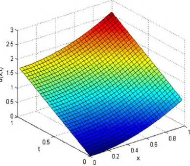
above problem is u(x,t) =x2+2Γ(α+1)

Γ(2α+1)t

2α_{. Figure 4 shows the exact solution for}

α =0.5. From figure 1 - 4, we can see that with J increasing, the numerical solution more and more close to the exact solution. Table 1, shows the absolute errors forα=0.5,t=0.5 and different values ofJ for example 1.

Figure 1.Numerical solution forJ = 4 Figure 2. Numerical solution forJ= 5

Figure 3.Numerical solution forJ = 6 Figure 4. Exact solution forα = 0.5

(11)

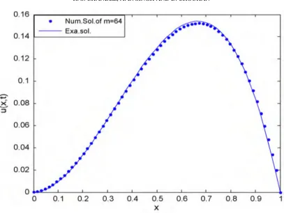
Example 2.Consider the space - time fractional convection - diffusion equation,

∂αu

∂tα =−b(x) ∂u

∂x+a(x) ∂βu ∂xβ

+q(x,t), 0≤x≤1, 0<t≤1

wherea(x) =Γ(2.8)₂x, b(x) =x0.8, q(x,t) =2x

2₍₁_−x₎_t1.2

Γ(2.2) +0.2x

1.8₍₁₊_t2₎_{and initial - boundary}

(12)

Figure 5.Comparison of numerical and exact solution fort=0.2 andJ=6.

Table 2.Exact solution att=0.2 and absolute error for different values ofJfor example 2.

(13)

This paper presents a numerical scheme based on Haar wavelets and operational matrices of fractional order integration for solving numerically FPDEs with variable coefficients supple-mented with initial and boundary conditions. The numerical examples show that the proposed method is very effective, accurate and easy to apply because it is computer oriented.

Conflicts of Interests

The authors declare that there is no conflict of interests. REFERENCES

[1] O. Abdulaziz, I. Hashim, E. S. Ismail, Approximate analytical solution to fractional modified KdV equations, Math. Comput. Model. 49 (2009), 136 - 145.

[2] C. F. Chen, C. H. Hsiao, Haar wavelet method for solving lumped and distributed - parameter systems, IEE Proc. Part D, 144 (1997), 87 - 94.

[3] Y. Li, W. Zhao, Haar wavelet operational matrix of fractional order integration and its applications in solving the fractional order differential equations, Appl. Math. Comput. 216 (2010), 2276 - 2285.

[4] K. Moaddy, S. Momani, I. Hashim, The non - standard finite difference scheme for linear fractional PDEs in fluid mechanics, Comput. Math. Appl. 61 (2011), 1209 - 1216.

[5] Z. M. Odibat, Rectangular decomposition method for fractional diffusion - wave equations, Appl. Math. Comput. 179 (2006), 92 - 97.

[6] Z. Odibat, S. Momani, A generalized differential transform method for linear partial differential equations of fractional order, Appl. Math. Lett. 21 (2008), 194 - 199.

[7] I. Podlubny, Fractional Differential Equations, Academic Press, San Diego, 1999.

[8] M. U. Rehman, R. A. Khan, A numerical method for solving boundary value problems for fractional differ-ential equations, Appl. Math. Modell. 36 (2012), 894 - 907.

[9] A. Saadatmandi, M. Dehghan, A new operational matrix for solving fractional - order differential equations, Comput. Math. Appl. 59 (2010), 1326 - 1336.

[10] J. Sabatier, O. P. Agrawal, J. A. Tenreiro Machado, Advances in Fractional Calculus: Theoretical Develop-ments and Applications in Physics and Engineering, Springer, 2007.