________________
*Corresponding author
Received August 31, 2016
1210 Available online at http://scik.org
J. Math. Comput. Sci. 6 (2016), No. 6, 1210-1220
ISSN: 1927-5307
NUMERICAL SOLUTIONS OF SECOND ORDER MATRIX DIFFERENTIAL EQUATIONS USING BASIS SPLINES
KAMAL R. M. RASLAN1 MOHAMED A. RAMADAN2,* AND MOHAMED A. SHAALAN3 1Faculty of science, Al-Azhar University, Cairo, Egypt
2Faculty of science, Menoufia University, Shebien El-Koom, Egypt 3Higher Technological Institute, Tenth of Ramadan City, Egypt
Copyright © 2016 Raslan, Ramadan and Shaalan. This is an open access article distributed under the Creative Commons Attribution License, which permits unrestricted use, distribution, and reproduction in any medium, provided the original work is properly cited.
Abstract. This paper aims to present a general framework of the cubic, quintic and septic B-splines functions to develop a numerical method for obtaining approximation solution numerical solution of the matrix differential equations of second order with boundary conditions. Numerical examples are included to illustrate the practical implementation of the proposed method. The results reveal that the proposed approach is very effective, convenient and quite accurate to such considered problems compared with cubic splines with constant term method.
Keywords: matrix differential equations; cubic b-splines; quintic b-splines; septic b-splines; Kronecker product; Frobenius norm.
2010 AMS Subject Classification: 35A24.
Introduction
Given the matrix boundary value problem
, ,
, , , R
,
a b
Y x f x Y x Y x
a x b a b
Y a Y Y a Y
(1)
where Y Y Y xa, b,
Cm n and matrix function f :
a b, Cm n Cm n Cm n , are frequent in different fields in physics and engineering. Equation (1) is similar to the statement of Newton’s law ofproblems with boundary value conditions [1- 6]. We define the Kronecker product of m n
AC
and BCp q , denoted by AB [7]
11 1
1
n
m mn
a B a B
A B
a B a B
(2)
The column vector operator on a matrix m n
AC is given by [7]:
1 Vec( )= ,
n
A A
A
where
1k k
mk
A A
A
(3)
If m n
YC and XCp q , then the derivative of a matrix with respect to a matrix is defined by [7]:
11 1
1
,
q
p pq
Y Y
x x
Y X
Y Y
x x
where
1 11
1
n
rs rs
rs
m mn
rs rs
Y Y
x x
Y x
Y Y
x x
(4)
If XCp q , YCq v and ZCm n , then the derivative of a matrix product with respect to another matrix is given by [7]:
,
n m
XY X Y
I Y I X
Z Z Z
(5)
where Im and In denote the identity matrices of dimensions m and n, respectively.
If XCp q , YCu v and ZCm n , then the chain rule is defined by [7]:
T
m q
Vec Y
Z Z
I I
X X Vec Y
(6)
and the derivative of a Kronecker product of matrices with respect to a matrix is given by [7]:
1 2
m n
X Y X Y
Y I U X I U
Z Z Z
(7)
where U1 and U2 are permutation matrices.
If ACm n , the frobenius norm of
A is given by [8]:
2 1 1 m n
ij F
i j
A a
(8)The following relationship between the 2-norm and frobenius norm holds [8]:
2 F 2
Cubic B - splines are used in [9-13], matrix differential equations are discussed in [14-16] and B-splines are presented in [17]. The paper is organized as follows: In section 2, we developed the
proposed method. In section 3, some numerical examples were discussed. Finally, in section 4, we gave summary of the suggested method.
2. Analysis of B-splines method
Let x0, , ..., x1 xN be
N1
grid points in the interval
a b, , sothatxi a ih i, 0, 1, ..., ; n x0a x, N b h,
b a
N. Then B-splines are presented as follows: 2.1 Cubic B-splinesThe cubic B-splines are
3
2 2 1
2 3
3 2
1 1 1 1
2 3
3 2
1 1 1 1
3
3 2
, ,
3 3 3 , ,
1
3 3 3 , ,
i i i
i i i i i
i i i i i i
i
x x x x
h h x x h x x x x x x
B x h h x x h x x x x x x
h
x x
1, 2 , 0 elsewhere.
i i
x x
i 1, 0,1,...,n1 .
(10)
We consider the B-spline function to the solutions
pq
x
y
of the problem (1):
1
1
; 1 , 1
pq pq pq N
i
x x x p n q m
i i
C
B
y
(11)where constants
pq
x i
C
’s are to be determined. To solve second order matrix boundary valueproblems, the
B B
i,
i andB
i at the nodal points are needed. Their coefficients are summarized in Table 1.Table 1. values of
B B
i, i andB
i.2
i
x xi1 xi xi1 xi2
i
B
0 1 4 1 0i
B
0 3 /h 0 3 /h 0i
B
0 26 /h 2
12 /h
2
6 /h 0
1 1 1
1 1 1
, , ,
pq pq pq pq pq pq
N N N
i i i
x x f x x x x x
i i i i i i
C
B
C
B
C
B
(12)and boundary conditions can be written as
1 1 1 1
; ,
; .
pq pq
N pq
a i
pq pq
N pq
b i
x x y x a
i i
x x y x b
i i
C
B
C
B
(13)
The spline solution of equation (1) is obtained by solving the following matrix equation. The
value of the spline functions at the points
0 N i i
x are determined using Table 1 and substitute into equations (12) and (13). Then a system q N
3
q N3 ; 1
q m of linear equations can be written as follows.
AEF (14)
Where,
11 11 11
1 0 1 1 0 1
11 11 11 11
0 0
, , , , , , , ,
, , , , , , , , , ,
T
nm nm nm
N N
T
nm nm nm nm
N N
a b a b
E C C C C C C
F y f x f x y y f x f x y
2.2 Quintic B-splines
The quintic B-splines are
5
3 3 2
5 5
3 2 2 1
5 5 5
3 2 1 1
5 5
3 2
5
, , 6 , ,
6 +15 , ,
1
6 +15
i i i
i i i i
i i i i i
i i i
x x x x
x x x x x x
x x x x x x x x
B x x x x x
h
5
1 1
5 5
3 2 1 2
5
3 2 3
, , 6 , , , , 0
i i i
i i i i
i i i
x x x x
x x x x x x
x x x x
elsewhere, i 1, 0,1,...,n 1 .
(15)
Let
2
2
; 1 , 1
pq pq pq N
i
x
C
i xB
i x p n q my
(16)be the B-spline function to the solutions
pq
x
where constants
pq
x i
C
’s are to be determined. To solve second order matrix boundary valueproblems, the
B B
i,
i andB
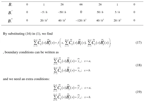
i at the nodal points are needed. Their coefficients are summarized in Table 2.Table 2. values of
B B
i, i andB
i.3 i
x xi2 xi1 xi xi1 xi2 xi3
i
B
0 1 26 66 26 1 0i
B
0 5 /h 50 /h 0 50 /h 5 /h 0i
B
0 220 /h 2
40 /h 2
120 /h
2
40 /h 2
20 /h 0
By substituting (16) in (1), we find
2 2 2
2 2 2
, , ,
pq pq pq pq pq pq
N N N
i i i
x x f x x x x x
i i i i i i
C
B
C
B
C
B
(17), boundary conditions can be written as
2 2 2 2
; ,
; .
pq pq
N pq
a i
pq pq
N pq
b i
x x y x a
i i
x x y x b
i i
C
B
C
B
(18)
and we need an extra conditions:
2 2 2 2
; ,
; .
pq pq
N pq
a i
pq pq
N pq
b i
x x y x a
i i
x x y x b
i i
C
B
C
B
(19)
The spline solution of equation (1) is obtained by solving the following matrix equation. The
value of the spline functions at the points
xi iN0 are determined using Table 2 and substitute intoequations (17 - 19). Then a system q N
5
q N5 ; 1
q m of linear equations can be written as follows.
AEF (20)
11 11 11
2 1 2 2 1 2
11 11 11 11 11 11
0 0
, , , , , , , ,
, , , , , , , , , , , , , ,
T
nm nm nm
N N
T
nm nm nm nm nm nm
N N
a a b b a a b b
E C C C C C C
F y y f x f x y y y y f x f x y y
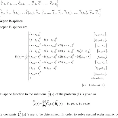
2.3 Septic B-splines
The septic B-splines are
7
4 4 3
7 7
4 3 3 2
7 7
4 3
7
, , 8 , ,
8 +28
1
i i i
i i i i
i i
i
x x x x
x x x x x x
x x x x x
B x h
7
2 2 1
7 7 7 7
4 3 2 1 1
7 7 7 7
4 3 2 1 1
7 7 7
4 3 2
, ,
8 +28 56 , ,
8 +28 56 , ,
8 +28
i i i
i i i i i i
i i i i i i
i i i
x x x
x x x x x x x x x x
x x x x x x x x x x
x x x x x x
1 2
7 7
4 3 2 3
7
4 3 4
, , 8 , , , , 0
i i
i i i i
i i i
x x
x x x x x x
x x x x
elsewhere,
i 1, 0,1,...,n1 .
(21)
The B-spline function to the solutions
pq
x
y
of the problem (1) is given as
3
3
; 1 , 1
pq pq pq N
i
x x x p n q m
i i
C
B
y
(22)where constants
pq
x i
C
’s are to be determined. In order to solve second order matrix boundaryvalue problems, the
B B
i,
i andB
i at the nodal points are needed. Their coefficients are summarized in Table 3.Table 3. values of
B B
i, i andB
i.4
i
x xi3 xi2 xi1 xi xi1 xi2 xi3 xi4
i
B
0 1 120 1191 2416 1191 120 1 0i
B
0 7 /h 392 /h 1715 /h 0 1715 /h 392 /h 7 /h 0i
B
0 242 /h 2
1008 /h 2
630 /h 2
3360 /h
2
630 /h 2
1008 /h 2
42 /h 0
i
B
0 3210 /h
3
1680 /h
3
3990 /h 0 3
3990 /h
3
1680 /h 3
By substituting (22) in (1), we find
3 3 3
3 3 3
, , ,
pq pq pq pq pq pq
N N N
i i i
x x f x x x x x
i i i i i i
C
B
C
B
C
B
(23), boundary conditions can be written as
3 3 3 3
; ,
; .
pq pq
N pq
a i
pq pq
N pq
b i
x x y x a
i i
x x y x b
i i
C
B
C
B
(24)
and we need an extra conditions:
3 3 3 3
; ,
; .
pq pq
N pq
a i
pq pq
N pq
b i
x x y x a
i i
x x y x b
i i
C
B
C
B
(25)
3 3 3 3
; ,
; .
pq pq
N pq
a i
pq pq
N pq
b i
x x y x a
i i
x x y x b
i i
C
B
C
B
(26)
The spline solution of equation (1) is obtained by solving the following matrix equation. The
value of the spline functions at the points
xi iN0 are determined using Table 3 and substitute intoequations (23 - 26). Then a system q N
7
q N7 ; 1
q m of linear equations can be written as follows.
AEF (27)
Where,
11 11 11
3 2 3 3 2 3
11 11 11 11 11 11 11 11
0 0
, , , , , , , ,
, , , , , , , , , , , , , , , , , ,
T
nm nm nm
N N
T
nm nm nm nm nm nm nm nm
N N
a a a b b b a a a b b b
E C C C C C C
F y y y f x f x y y y y y y f x f x y y y
3. Numerical examples
In this section, we present some examples of matrix differential equations of second order. We
between approximate solution and exact solution, and then take the Frobenius norm of this difference.
Example 1. A non-linear differential vector system [16] Let
21 21 2 2 111 cos sin cos
, 0 1.
1 1
4 5 sin
x y x y x
Y x x
y x x
(28)
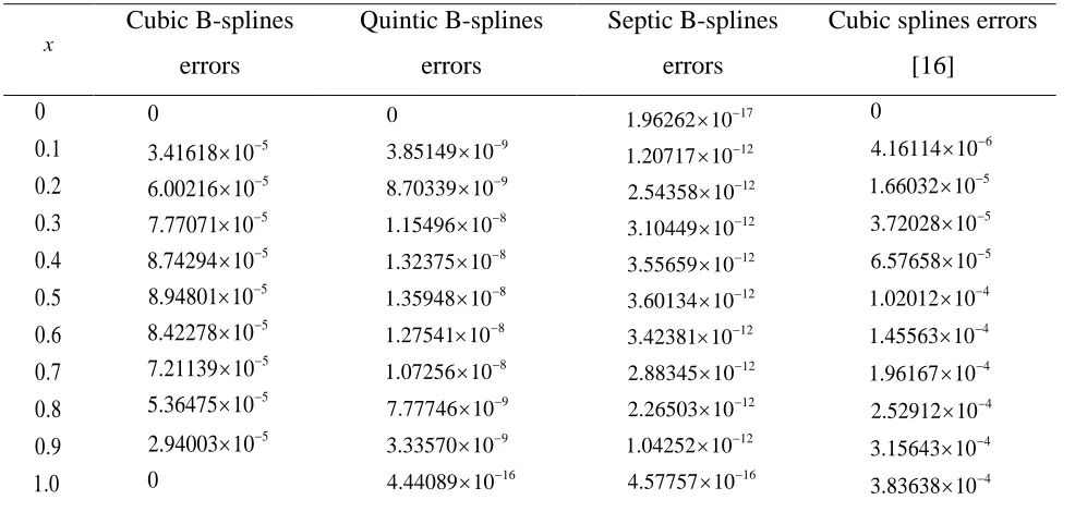
This example has an exact solution Y x
cos
x x
. Thus, we can compare our numerical
estimates with this solution to obtain the exact errors of the approximation which summarized in Table 4.
Table 4. Approximation for Example 1.
x Cubic B-splines errors Quintic B-splines errors Septic B-splines errors
Cubic splines errors [16] 0 0.1 0.2 0.3 0.4 0.5 0.6 0.7 0.8 0.9 1.0 5 5 5 5 5 5 5 5 5 3.41618 10 6.00216 10 7.77071 10 8.74294 10 8.94801 10 8.42278 10 7.21139 10 5.36475 10 2.94003 1 0 0 0 9 9 8 8 8 8 8 9 9 16 0 3.85149 10 8.70339 10 1.15496 10 1.32375 10 1.35948 10 1.27541 10 1.07256 10 7.77746 10 3.33570 10 4.44089 10 17 12 12 12 12 12 12 12 12 12 16 1.96262 10 1.20717 10 2.54358 10 3.10449 10 3.55659 10 3.60134 10 3.42381 10 2.88345 10 2.26503 10 1.04252 10 4.57757 10 6 5 5 5 4 4 4 4 4 4 4.16114 10 1.66032 10 3.72028 10 6.57658 10 1.02012 10 1.45563 10 1.96167 10 2.52912 10 3.15643 10 3.83638 10 0
Example 2. Incomplete second - order differential system [16] The problem
0, 0 1.Y x AY x x (29)
Where 1 0
2 1
A
and corresponding exact solution
sin 0 cos sin x Y xx x x
. Thus, we can find
Table 5. Approximation for Example 2.
x Cubic B-splines
errors
Quintic B-splines errors
Septic B-splines errors
Cubic splines errors [16] 0 0.1 0.2 0.3 0.4 0.5 0.6 0.7 0.8 0.9 1.0 17 5 4 4 4 4 4 4 4 4 15 1.20185 10 7.86131 10 1.51856 10 2.14489 10 2.61535 10 2.88399 10 2.90988 10 2.65820 10 2.10116 10 1.21887 10 2.11526 10 15 8 8 8 8 8 8 8 8 8 16 5.48450 10 1.21289 10 2.96468 10 4.30700 10 5.34986 10 5.92703 10 5.96807 10 5.35877 10 4.14174 10 1.86540 10 1.57009 10 15 12 11 11 11 11 11 11 11 12 16 4.01297 10 4.88643 10 1.11081 10 1.49671 10 1.85289 10 2.02749 10 2.07159 10 1.86006 10 1.56682 10 7.56441 10 1.11022 10 6 6 5 5 5 4 4 4 4 4 1.0072 10 6.3032 10 2.0059 10 4.6213 10 8.8359 10 1.4964 10 2.3267 10 3.3941 10 4.7114 10 6.28 0 38 10
Example 3. Second - order polynomial matrix equation [16] We consider the following problem
0
1
0, 0 1.Y x A Y x AY x x (30)
where 0 1
1 1 0 0
,
0 2 0 1
A A
and the exact solution
1 0
x x x
x
e e xe
Y x
e
. Thus, we
summarized the exact errors at each point in Table 6.
Table 6. Approximation for Example 3.
x Cubic B-splines
errors
Quintic B-splines errors
Septic B-splines errors
4. Conclusion
In this paper, we presented a numerical treatment for the second-order matrix differential
equations using B-spline functions of different types. The computational results are found to be in good agreement with the exact solutions by finding frobenius norm and are compared with Ref. [16] as shown in Tables 4, 5 and 6.
Conflict of Interests
The authors declare that there is no conflict of interests.
REFERENCES
[1] P. Marzulli, Global error estimates for the standard parallel shooting method, J. Comput. Appl. Math. 34 (1991), 233–241.
[2] J. M. Ortega, Numerical analysis: A second course, Academic Press, New York, 1972.
[3] B. W. Shore, Comparison of matrix methods to the radii Schrodinger eigenvalue equation: The Morse potential¨ , J. Chemical Physics 59 (1971 ), no. 12, 6450–6463.
[4] C. Froese, Numerical solutions of the hartree-fock equations, Can. J. Phys. 41 (1963 ), 1895–1910.
[5] J. R. Claeyssen, G. Canahualpa, and C. Jung, A direct approach to second-order matrix non-classical vibrating equations, Appl. Numer. Math. 30 (1999 ), 65–78.
[6] J. F. Zhang, Optimal control for mechanical vibration systems based on second-order matrix equations, Mechanical Systems and Signal Processing 16 (2002 ), no. 1, 61–67.
[7] A. Graham, Kronecker products and matrix calculus with applications, John Wiley, New York, 1981.
[8] G. H. Golub and C. F. Van Loan, Matrix computations, second ed., The Johns Hopkins University Press, Baltimore, MD, USA, 1989.
[9] F. R. Loscalzo and T. D. Talbot, Spline function approximations for solutions of ordinary differential equations, SIAM J. Numer. Anal. 4 (1967), no. 3, 433–445.
[10] E. A. Al-Said, The use of cubic splines in the numerical solution of a system of second-order boundary value problems, Comput. Math. Appl. 42 (2001), 861–869.
[11] M. K. Kadalbajoo and K. C. Patidar, Numerical solution of singularly perturbed two-point boundary value problems by spline in tension, Appl. Math. Comput. 131 (2002), 299–320.
[12] E. A. Al-Said and M. A. Noor, Cubic splines method for a system of third-order boundary value problems, Appl. Math. Comput. 142 (2003), 195–204.
[13] G. Micula and A. Revnic, An implicit numerical spline method for systems for ODE’s, Appl. Math. Comput. 111 (2000), 121–132.
[15] E. Defez, L. Soler, A. Hervas, and M. M. Tung, Numerical solutions of matrix differential models using cubic matrix splines II, Mathematical and Computer Modelling 46 (2007), 657–669.
[16] M. M. Tung, E. Defez, and Sastre, Numerical solutions of second-order matrix models using cubic-matrix splines, Computers and Mathematics with Applications 56 (2008) 2561–2571.