Reliability Assessment of Bearings Based on Performance Degradation Values under Small Samples

0 INTRODUCTION

Bearings, a highly common and essential machine part, play a significant impact on machines’ performance. Obviously, the lifetime of machines heavily depends on the lifetime of bearings. In recent years, the quality and reliability of the products have been increasingly emphasized. Douglas [1] pointed out the value of the reliability in electricity power. Zio [2] listed the old problems and new challenges in reliability engineering and gave some remarks on the future needs for the practice of it. Researchers have proposed various methods to assess the reliability of different products. Gao et al. [3] developed dynamic reliability models for mechanical components with a failure model of fatigue. Ognjanovic and Milutinovic [4] designed a methodology for automotive gearbox load capacity identification based on the requirement of reliability. Bicek et al. [5] inspected the most likely potential mechanical causes of failure modes for in-wheel motors. Rashid et al. [6] applied the influence diagram to establish the reliability model for a helicopter main gearbox lubrication system. The working situation of the products with high reliability, like long lifetime bearings, cannot be simply described with normal 1 and failure 0, however. It can be represented by the performance of the products during operating time. Therefore, the reliability assessment

method based on performance degradation data has been developed. The performance degradation data of bearings has been applied in the reliability assessment in recent years. Support vector machine (SVM) and the Markov model were applied in the prediction of bearings’ degradation process [7]. Zhang et al. [8] discussed how to choose the degradation feature of bearings to predict the remaining life of the bearings. Some other researchers [9] identified the degradation of bearings by the relevance vector machine. Many engineering and technical personnel and statistical scholars attempted to analyse products’ reliability based on performance degradation data and achieved success in theoretical research and engineering application according to [10] and [11]. Pan [12] applied gamma processes in reliability assessment based on the degradation data of products.

In research studies that involve the content of reliability evaluation based on degradation data, the distribution-based degradation method is one that has been widely accepted. The distribution-based degradation method was taken into the reliability assessment, and satisfying results were obtained in literature [13] to [15]. The key step of the method is to calculate the estimation of the distribution parameters at every moment. However, the estimation method is suitable for large sample situations but is not entirely appropriate for small samples.

Reliability Assessment of Bearings Based on Performance

Degradation Values under Small Samples

Qin, L. – Shen, X. – Chen, X – Gao, P.

Luosheng Qin – Xuejin Shen* _{– Xiaoyang Chen – Pandong Gao}

Shanghai University, School of Mechatronic Engineering and Automation, China

It is difficult to obtain the lifetime data of a long lifetime bearing from a test with limited time. Therefore, to apply the method of reliability assessment based on lifetime data to the high reliability and long lifetime bearings would be impractical. The performance degradation data, which containsreliability information, could be used in the reliability assessment. However, the methods based on performance degradation data are often applied in a large sample situation. In this paper, a method suitable for a small-sample situation based on a distribution-based degradation model and a bootstrapping method combined with the Monte Carlo method (DDBMC) is proposed. This method is put forward to enlarge the sample size and estimate the distribution parameters. Then, the function between distribution parameters and time can be obtained by using the least square method. In this paper, the reliability of the ball bearings under a small sample is assessed to verify the proposed method. Finally, the proposed methodology was applied to assessing the reliability of bearings and shown to be efficient in the reliability assessment of bearings under small samples.

Keywords: bearings, distribution-based degradation, small sample, bootstrapping method, Monte Carlo method, reliability

Highlights

• The reliability of bearings has been assessed based on the degradation data.

• Reliability of bearings has been revaluated by the distribution-based degradation method. • Parameters of the distribution has been estimated under small samples.

Nowadays, the problem of small datasets is attracting increasing attention. Bootstrapping [16] is a good method to enlarge the sample sizes. Many engineers and scholars use it to raise the precision of the parameters’ estimation. Structural reliability was assessed by applying the bootstrapping method, according to [17]. Li et al. [18] pointed out that the method was useful for statistics with an unknown distribution and datasets with small sample size. The Bootstrapping method and Monte Carlo simulation were applied to evaluating the uncertainty of failure rate estimation in engineering problems [19]. The Monte Carlo method is another widely used method in engineering and statistics. That method and fault tree analysis were applied to analysis of the reliability for a wastewater treatment plant [20]. The Monte Carlo simulation was also applied to the solution of the population balance equations, and the accuracy and the optimal sampling in Monte Carlo solutions of the equations have been discussed [21]. A multilevel Monte Carlo method was proposed to estimate the uncertainty in pore-scale and digital rock physics problems [22].

In this paper, a reliability assessment method, which is combined with the Monte Carlo method on the basis of distribution-based degradation method and bootstrapping method, is put forward to evaluate the reliability of bearings under small samples. To describe the method conveniently, the proposed method, i.e. reliability assessment method based on the distribution of distribution-based degradation method and bootstrapping method combined with Monte Carlo method, is called DDBMC. At the end of the paper, the proposed method was applied to assess the reliability of bearings. The DDBMC method can make full use of the performance degradation data and obtain relatively accurate results.

1 THE BASIC THEORY OF DDBMC

The distribution-based degradation method is widely used in reliability evaluation based on degradation data. The operation is simple and convenient for

engineering applications, and the basic principle is

described as follows.

Suppose there are n samples in the test, and a

performance y during the test is recorded at every

moment tj ( j = 1, 2, ..., m, m is a positive integer), the

matrix of performance degradation data is written as Eq. (1).

y

y y y y

y y y y

y y m m m m n n = − − − −

1 1 1 2 1 1 1

2 1 2 2 2 1 2

1 1 1 2

, , , , , , , , , , yy y

yn yn yn mn m yn mn m

− − − −                

1 1 1

1 2 1

, ,

, , , ,

.

(1)

The distribution hypothesis testing for each column of the matrix Eq. (1) should be carried out first. According to the common practice in the literature, the normal distribution function is widely selected. In this paper, the K-S hypothesis testing method is applied to verify whether the performance degradation data at every moment follow a normal distribution or not. After that, the corresponding parameters of the distribution function are estimated.

If the performance degradation data y at each

time follows the normal distribution, the distribution

parameters at each detection time tj in Eq. (1) are

calculated by applying Eq. (2).

µ_{j ij} σ µ

i n

j _{ij j}

i n

n y n y

= = − − = =

∑

∑

1 1 1 1 1 2

, ( ) , (2)

where i represents the sample identification,

i = 1, 2, …, n, j represents the order of recording time,

j = 1, 2, …, m, µ_{j ij} σ µ

i n

j _ij j

i n

n y n y

= = − − = =

∑

∑

1 1 1 1 1 2 , ( ) , and

µ_{j ij} σ µ

i n

j _ij j

i n

n y n y

= = − − = =

∑

∑

1 1 1 1 1 2

, refer to the parameter ( ) ,

estimates of normal distribution.

When the parameters estimated at each moment were obtained, the optimal function between parameter and operating time could be easily evaluated by applying the least square method, and

the optimal function of µ_{j ij} σ µ

i n

j _{ij j}

i n

n y n y

= = − − = =

∑

∑

1 1 1 1 1 2 , ( ) , and

µ_{j ij} σ µ

i n

j _{ij j}

i n

n y n y

= = − − = =

∑

∑

1 1 1 1 1 2

, can be written as ( ) ,

µ_{j ij} σ µ

i n

j _{ij j}

i n

n y n y

= = − − = =

∑

∑

1 1 1 1 1 2 , ( ) ,

(tj) and

µ_{j ij} σ µ

i n

j _{ij j}

i n

n y n y

= = − − = =

∑

∑

1 1 1 1 1 2

, (tj). Then, the reliability estimation ( ) , R t( )_j

at any time tjis:

R t l t

t j j j    ( ) ( ( ) ( ) ), =Φ −µ

σ (3)

where l represents the products’ performance

degradation threshold and Φ refers to standard normal distribution function.

1.1 Estimation Method under Small Samples

The bootstrapping method combined with Monte Carlo method (BMC) is put forward to estimate parameters under small datasets. First, the Monte Carlo method is applied to simulate new data from the original data. After that, the bootstrapping method is applied to estimate the parameters.

Obtaining these numbers is the process called “generation of random numbers” [23]. A data-based random number simulation method is mentioned

in [24] and the method could accurately obtain the

variance of the sample. The process is expressed as follows:

a) Randomly choose a point, xj, from the given

sample.

b) Identify the m nearest neighbours of xj (including

xj), xj1, xj2, ..., xjm, and determine their mean, xj.

c) Generate a random sample, u1, u2, ..., um, from a uniform distribution with:

lower bound 1 m− 3(m−1) m2 and

upper bound 1 m+ 3(m−1) m2 .

d) Deliver the random variate

z u x_{k jk} x_j x

k m j = − + =

∑

( ) . 1 (4)

The simulation data at each moment tj could be

obtained by the computer according to the above steps.

In this paper, m equals the original sample number,

and the steps a) to d) are repeated for m times. According to Eq. (4), estimation of parameters at every moment tj can be referred as Eq. (5):

µ_{Mj i} σ µ

i m

Mj _i Mj

i m

m z m z

i m j

= = − − = = = =

∑

∑

1 1 1 1 2 1 2

1 1

2

, ( ) ,

, , ..., , , , ...., ,n (5)

where m represents the simulation sample number, j

represents the number of recording time, j = 1, 2, ..., n,

µ_{Mj i} σ µ

i m

Mj _{i Mj}

i m

m z m z

i m j

= = − − = = = =

∑

∑

1 1 1 1 2 1 2

1 1

2

, ( ) ,

, , ..., , , , ...., ,n

and

µ σ µ

_Mj  

i i

m

Mj _i Mj

i m

m z m z

i m j

= = − − = = = =

∑

∑

1 1 1 1 2 1 2

1 1

2

, ( ) ,

, , ..., , , , ...., ,n

refer to the normal distribution parameter estimates of simulated data.

According to the bootstrapping method, this process would be repeated for B times. In this paper, B

is set as 10000, and B groups of µ_{Mj i} σ µ

i m

Mj _{i Mj}

i m

m z m z

i m j

= = − − = = = =

∑

∑

1 1 1 1 2 1 2

1 1

2

, ( ) ,

, , ..., , , , ...., ,n

(k) and

µ_{Mj i} σ µ

i m

Mj _{i Mj}

i m

m z m z

i m j

= = − − = = = =

∑

∑

1 1 1 1 2 1 2

1 1

2

, ( ) ,

, , ..., , , , ...., ,n

(k)

(k = 1, 2, ..., B) are obtained at time tj. The final

estimation results of distribution parameters are calculated as shown in Eqs. (6) and (7).

µ µ µ

  

BMj oj Mj k

k B B = − =

∑

2 1 1

( ), (6)

σBMj σoj σMj k k B B 2 2 2 1 2 1 = − =

∑

( ( )) . (7)

In Eq. (6), µ_BMj µ_oj µ_{Mj k}

k B B = − =

∑

2 1 1 ( ), and

σBMj σoj σMj k k B B 2 2 2 1 2 1 = − =

∑

( ( )) .

stand for the parameters of original samples and k = 1, 2, ..., B. Final estimation results of distribution parameters µ_BMj µ_oj µ_{Mj k}

k B B = − =

∑

2 1 1 ( ), BMj and

σBMj σoj σMj k k B B 2 2 2 1 2 1 = − =

∑

( ( )) .

BMj at

every time are calculated by the method proposed. The reliability assessment method based on distribution of performance degradation values deems that distribution parameters are functions of time t, so

the function expressions µ( )_{t e}. . ,

j and = 0 00061 1 2323σ( )tt−j are easily =e0 00064. t−. .1 4095.

gotten according to the estimation results µ_BMj µ_oj µ_{Mj k}

k B B = − =

∑

2 1 1 ( ), BMj and

σBMj σoj σMj k k

B

B

2 2 ₂

1 2 1 = − =

∑

( ( )) .

BMj of distribution parameters at every moment.

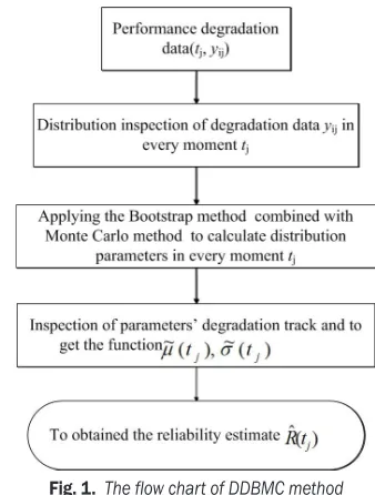
1.2 Analysis Process of DDBMC method

At every moment tj , the test data, i.e. a column of

the matrix as Eq. (1), often belongs to the same distribution function family. And parameters of the distribution can be easily estimated. In this paper, in order to solve the problem of small sample, the bootstrapping method combined with Monte Carlo method is introduced. The concrete process of this method is shown in Fig. 1.

Fig. 1. The flow chart of DDBMC method

1.3 Validation of the Proposed Method

To verify the correctness and applicability of this method under a small sample situation, a set of bearings’ degradation data is given. The data are analysed by applying the DDBMC method.

The test was carried out under the sample size

n = 7, and the censoring time of the test was set at 4000 h. According to the requirements of the test, the axial load was set at 5 N, and the test speed was 58000 rpm. Before the formal test, the bearings were required to be run 3 hours under 1/2 test speed.

survived. The operating time of the samples is listed in Table 1.

The lifetimes of the samples were assumed to follow the Weibull distribution. The traditional method, based on lifetime data and maximum likelihood estimation (MLE), was applied to the analysis of the data in Table 1. In Table 1, the status “F” stands for failure and the status “S” stands for survive. The Weibull distribution function is shown as follows.

F x( )= −exp −t ,



 

  

  



  

1

η

β

(8)

where β stands for the shape parameter, and η stands for the scale parameter. It is supposed that the operating time data is recorded as t(1) ≤ t(2) ≤ ... ≤ t(n). The shape parameter and the scale parameter are calculated by the following equation [25]:

1

0

1

1

1

1

1 β

λ

λ

η

λ

β

β

β β

+ − =

=

=

=

=

=

=

∑

∑

∑

∑

∑

i i i

n

i i

n

i i

i n

i i

n

i i

n

i i

t t t

t

t

ln ln

==

∑



    

    

 1

n

. (9)

In Eq. (9), if ti stands for the lifetime (the status

F), then λi = 1, else λi = 0. The MLE estimates of

Weibull shape and scale parameters are 3.5699 and

3175.8909, respectively. Reliability estimation results are listed in Table 2 and shown in Fig. 2. In Table 2, “R” stands for the reliability estimation.

The bearings’ vibration responses of the first 1300 h, which are recorded every 130 h, are listed in Table 3.

Hypothesis testing is put forward to verify the distribution of the data in Table 3. According to the K-S hypothesis testing method, under the condition of the significance level 0.05, the H value indicates whether to accept the hypothesis testing. H = 0 refers to accepting it and H = 1 refers to declining it. The results of Hypothesis testing show that the performance degradation data at every moment in Table 3 follow the normal distribution.

Table 1. Operating times of the samples

Sample No. 1 2 3 4 5 6 7

Status F F F F F S S

Operating

time [h] 1313 2288 2472 2506 3382 4000 4000

According to the vibration data in Table 3 and the DDBMC method, mean µ_BMj µ_oj µ_{Mj k}

k B

B

= −

=

∑

2 1

1 ( ),

BMj and standard deviation

σBMj σoj σMj k k

B

B

2 2

2

1

2 1

= −

=

∑

( ( )) .

BMj of the samples at every moment are calculated,

as shown in Table 4. An exponential model or a linear model are used to describe the degradation path of bearings, as suggested by [26] and [27]; the exponential model shows the better fit according to [28]. Next, µ_BMj µ_oj µ_{Mj k}

k B

B

= −

=

∑

2 1

1 ( ),

BMj and

σBMj σoj σMj k k

B

B

2 2

2

1

2 1

= −

=

∑

( ( )) .

BMj are supposed to be fitted by the

exponential function, and the functions are obtained as Eqs. (10) and (11).

Table 2. The reliability estimation results of the first 1300 h by applying MLE

t [h] 100 300 500 700 900 1100 1300

R 0.9999 0.9998 0.9986 0.9955 0.9890 0.9775 0.9596

Table 3. Vibration responses of bearings [g] Sample

Time [h] 1 2 3 4 5 6 7

0 0.0300 0.0870 0.0841 0.1825 0.0020 0.1163 0.0916

130 0.1850 0.4940 0.1484 0.9687 1.0516 0.4674 0.1134

260 0.2220 0.2870 0.1658 1.1680 0.9137 0.7572 0.1468

390 0.2565 0.3038 0.1585 1.1959 0.9469 0.7512 0.1195

520 0.1704 0.2750 0.1643 0.6521 1.5600 0.4170 0.1579

650 0.1900 0.8104 0.1453 1.0110 1.2832 0.6474 0.1725

780 0.2189 0.6368 0.1583 0.8428 0.9030 0.8203 0.1807

910 0.2044 0.5421 0.1885 0.5057 1.0055 0.2988 0.1894

1040 0.2244 0.6117 0.1466 0.5812 1.2964 0.5471 0.1458

1170 0.2256 0.4064 0.1825 0.3686 1.2808 0.6115 0.1338



µ( )t_j =e0 00061 1 2323. t−. , (10)



σ( )t e. . . .

j = 0 00064t−1 4095 (11)

Then taking Eqs. (10) and (11) into Eq. (3), and the reliability estimates are listed in Table 5 and plotted in Fig. 2.

As shown in Fig. 2, it can be found that the estimation results with the DDBMC method are close to the results estimated by MLE and tend to be conservative. This illustrates the applicability of the method under small sample and the advantages of the DDBMC method in reliability assessment based on performance degradation under small samples.

Table 4. Sample mean and standard deviation of the vibration responses at different times [g]

Parameter

Time [h] µBMj µoj µMj k k

B

B

= −

=

∑

2 1

1 ( ),

BMj σBMj σoj σMj k k

B

B

2 2 ₂

1

2 1

= −

=

∑

( ( )) .

BMj

0 0.0846 0.0635

130 0.4906 0.4218

260 0.5230 0.4543

390 0.5314 0.4676

520 0.4856 0.5516

650 0.6085 0.4955

780 0.5374 0.3701

910 0.4192 0.3253

1040 0.5070 0.4416

1170 0.4608 0.4336

1300 0.5540 0.4886

Table 5. The reliability estimation results of the first 1300 h by applying DDBMC

t [h] 700 900 1100 1300

R 0.9975 0.9907 0.9701 0.9363

Fig. 2. The reliability estimation comparison between MLE and DDBMC method

2 RELIABILITY ANALYSIS OF BEARINGS

The DDBMC method is applied in assessing the reliability of bearings in this section. The test is carried out with the sample size n = 8, and the censoring time is set at 4000 h. The test speed is 5100 rpm. According to the requirements of the bearing manufacturer and customers, the test failure criterion is defined as: bearings’ vibration responses reach 6 dB higher than the initial values. The increased value of the bearings’ vibration at every measurement point is recorded in Table 6.

Before processing the data in Table 6, the K-S hypothesis testing method is also applied. According to the K-S hypothesis testing method, the performance degradation data at the same moment follow the normal distribution.

According to the vibration data in Table 6 and the

DDBMC method, mean µ_BMj µ_oj µ_{Mj k}

k B

B

= −

=

∑

2 1

1 ( ),

BMj and and standard

Table 6. The increased value of the bearings’ vibration [dB] Sample

Time [h] 1 2 3 4 5 6 7 8

447 1.17 0 0 0 0 0 0 0

1119 1.17 0.33 0 0 0 0 0 0

1503 0 0.33 2.58 0 0 0.37 0.53 1.99

1911 0 0 2.58 0 0 0.37 1.88 1.99

2511 0 0 2.58 0 1.1 0.37 0 0.27

2679 0 1.48 2.58 0 0 2.61 0.53 0

3015 1.17 0.33 1.12 0 0 0.37 1.88 1.99

3279 0 1.48 1.12 0 0 0.37 0 1.99

3687 1.17 0.34 1.12 0 2.3 0.37 0 1.99

3911 0 1.48 0 0 2.3 3.69 0 1.99

deviation σBMj σoj σMj k k

B

B

2 2 ₂

1

2 1

= −

=

∑

( ( )) .

BMj of the samples at every moment are

listed in Table 7. The function expressions as Eqs. (12) and (13) are obtained from the results in Table 7.



µ( )_{t e}. . ,

j = 0 00043 1 6213t− (12) 

σ( )t_j =e0 00025. t−0 6985. . (13)

Next, by taking Eqs. (12) and (13) into Eq. (3), reliability estimates can be plotted in Fig. 3. Reliability estimates in the 5000 h are listed in Table 8.

As shown in Fig. 3, the rating life of the bearings is about 6720 h, which means the reliability of the bearings is 0.9 at about 6720 h under the test condition. It could also be found in Fig. 3 that the lifetime data is difficult to obtain in this situation while the proposed DDBMC method demonstrates effectiveness to solve the problem.

Fig. 3. Reliability estimation of the bearings

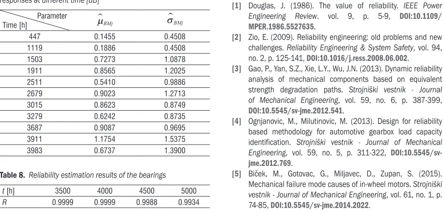
Table 7. Sample mean and standard deviation of the vibration responses at different time [dB]

Parameter

Time [h] µBMj µoj µMj k k

B

B

= −

=

∑

2 1

1 ( ),

BMj σBMj σoj σMj k k

B

B

2 2

2

1

2 1

= −

=

∑

( ( )) .

BMj

447 0.1455 0.4508

1119 0.1886 0.4508

1503 0.7273 1.0878

1911 0.8565 1.2025

2511 0.5410 0.9886

2679 0.9023 1.2713

3015 0.8623 0.8749

3279 0.6242 0.8735

3687 0.9087 0.9695

3911 1.1754 1.5375

3983 0.6737 1.3900

Table 8. Reliability estimation results of the bearings

t [h] 3500 4000 4500 5000

R 0.9999 0.9999 0.9988 0.9934

3 CONCLUSIONS

It is impractical to analyse the reliability of bearings based on lifetime data because of the difficulty of obtaining highly reliable bearing data. Reliability analysis based on performance degradation data solves the problem of reliability assessment without lifetime data, although, the existing performance degradation method cannot obtain the ideal results under small samples. In this paper, a method called DDBMC is proposed to solve this problem, and it is suitable for assessing the reliability of products with high reliability under small data sets.

In addition, the method of generating simulated data used in this article completely depends on the test sample data, which can simultaneously retain the original nature of the sample data and expand the original data. Finally, the results under small sample are close to the real situation.

To summarize, the DDBMC method can evaluate the reliability under small samples without lifetime data. However, it should be pointed out that the DDBMC method considers only the small sample problem and ignores the problem of little measurement point, which still needs further study.

4 ACKNOWLEDGEMENT

This work is carried out with financial support from the National twelfth five-year projects of China for science and technology under Contract D.50-0109-15-001 and D.71-0109-16-046.

5 REFERENCES

[1] Douglas, J. (1986). The value of reliability. IEEE Power Engineering Review. vol. 9, p. 5-9, DOI:10.1109/

MPER.1986.5527635.

[2] Zio, E. (2009). Reliability engineering: old problems and new challenges. Reliability Engineering & System Safety, vol. 94, no. 2, p. 125-141, DOI:10.1016/j.ress.2008.06.002.

[3] Gao, P., Yan, S.Z., Xie, L.Y., Wu, J.N. (2013). Dynamic reliability analysis of mechanical components based on equivalent strength degradation paths. Strojniški vestnik - Journal of Mechanical Engineering, vol. 59, no. 6, p. 387-399,

DOI:10.5545/sv-jme.2012.541.

[4] Ognjanovic, M., Milutinovic, M. (2013). Design for reliability based methodology for automotive gearbox load capacity identification. Strojniški vestnik - Journal of Mechanical Engineering, vol. 59, no. 5, p. 311-322,

DOI:10.5545/sv-jme.2012.769.

[6] Rashid, H.S.J., Place, C.S., Mba, D., Keong, R.L.C., Healey, A., Kleine-Beek, W., Romano, M. (2015). Reliability model for helicopter main gearbox lubrication system using influence diagrams. Reliability Engineering & System Safety, vol. 139, p. 50-57, DOI:10.1016/j.ress.2015.01.021.

[7] Dong, S.J., Yin, S.R., Tang, B.P., Chen, L.L., Luo, T.H. (2014). Bearing degradation process prediction based on the support vector machine and Markov model. Shock and Vibration, vol. 2014, p. 1-14, DOI:10.1155/2014/717465.

[8] Zhang, B., Zhang, L.J., Xu, J.W. (2016). Degradation feature selection for remaining useful life prediction of rolling elements bearings. Quality and Reliability Engineering International, vol. 32, no. 2, p. 547-554, DOI:10.1002/qre.1771.

[9] Caesarendra, W., Widodo, A., Thom, P.H., Yang, B.S., Setiawan, J.D. (2011). Combined probility approach and indirect data-driven method for bearing degradation prognostics. IEEE Transactions on Reliability, vol. 60, no. 1, p. 14-20,

DOI:10.1109/TR.2011.2104716.

[10] Lu, J.C., Meeker, W.Q. (1993). Using degradation measures to

estimate a time-to-failure distribution. Technometrics, vol. 35, no. 2, p. 161-174, DOI:10.2307/1269661.

[11] Crk, V. (2000). Reliability assessment from degradation

data. Annual Proceedings of Reliability and Maintainability Symposium, p. 155-161, DOI:10.1109/RAMS.2000.816300.

[12] Pan, Z., Balakrishnan, N. (2011). Reliability modeling

of degradation of products with multiple performance characteristics based on gamma processes. Reliability Engineering & System Safety, vol. 96, no. 8, p. 949-957,

DOI:10.1016/j.ress.2011.03.014.

[13] Li, C.Q. (1995). Computation of the failure probability of

deteriorating structural systems. Computers & Structures, vol. 56, no. 6, p. 1073-1079, DOI:10.1016/0045-7949(94)00947-2.

[14] Yang, K., Xue, J.N. (1996). Continuous state reliability analysis. Proceedings Annual of the Reliability and Maintainability Symposium, p. 251–257.

[15] Chen, Y.X., Zeng, Z.G., Kang, R. (2012). Validation methodology

for distribution-based degradation model. Journal of System Engineering and Electronics, vol. 23, no. 4, p. 553-559,

DOI:10.1109/JSEE.2012.00069.

[16] Efron, B. (1979). Bootstrap methods: Another look at the

Jackknife. The Annals of Statistics, vol. 7, no. 1, p. 1-26,

DOI:10.1214/aos/1176344552.

[17] Chaves, I.A., Machado, P.D., Neto, A.C. (2014). Estimation

of failure probability in corroded oil pipelines through Monte Carlo simulation method applying the Bootstrap technique.

International Journal of Applied Science and Technology, vol. 4, no. 5, p. 141-152.

[18] Li, D.Q., Tang, X.S., Zhou, C.B., Phoon, K.K. (2015).

Characterization of uncertainty in probabilistic model using bootstrap method and its application to reliability of piles. Applied Mathematical Modeling, vol. 39, no. 17, p. 5310-5326, DOI:10.1016/j.apm.2015.03.027.

[19] Kumar, B., Datta, D. (2010). Estimation of probability of

failure using bootstrap methods. International Conference on Reliability, Safety and Hazard, p. 143-146, DOI:10.1109/

ICRESH.2010.5779532.

[20] Taheriyoun, M., Moradinejad, S. (2015). Reliability analysis of a wastewater treatment plant using fault tee analysis and Monte Carlo simulation. Environmental Monitoring and Assessment, vol. 187, p. 1-13, DOI:10.1007/s10661-014-4186-7.

[21] Yu, X., Hounslow, M.J., Reynolds, G.K. (2015). Accuracy and

optimal sampling in Monte Carlo solution of population balance equation. AIChE Journal, vol. 61, no. 8, p. 2394-2402,

DOI:10.1002/aic.14837.

[22] Icardi, M., Boccardo, G., Tempone, R. (2016). On the

predictivity of pore-scale simulations: Estimating uncertainties with multilevel Monte Carlo. Advances in Water Resources, vol. 95, p. 46-60, DOI:10.1016/j.advwatres.2016.01.004.

[23] Gentle, J.E. (2009). Computational Statistics. Springer,

Dordrecht, DOI:10.1007/978-0-387-98144-4.

[24] Taylor, M.S., Thompson, J.R. (1986). A data based algorithm

for the generation of random vectors. Computational Statistics & Data Analysis, vol. 4, no. 2, p. 93-101,

DOI:10.1016/0167-9473(86)90013-7.

[25] Kahle, W. (1996). Estimation of the parameters of the Weibull

distribution for censored samples. Metrika, vol. 44, no. 1, p. 27-40, DOI:10.1007/BF02614052.

[26] Shao, Y., Nezu, K. (2000) Prognosis of remaining bearing

life using neural networks. Proceedings of the Institution of Mechanical Engineers, Part I: Journal of Systems and Control Engineering, vol. 214, no. 3, p. 217-230,

DOI:10.1243/0959651001540582.

[27] Gebraeel, N., Lawley, M., Liu, R., Parmeshwaran, V. (2004)

Residual life predictions from vibration-based degradation signals: A neural network approach. IEEE Transactions on Industrial Electronics, vol. 51, no. 3, p. 694-700, DOI:10.1109/

TIE.2004.824875.