Vol 5, No. 1, (2015), pp 73-83
Numerical solution of damped forced
oscillator problem using Haar wavelets
I. Singh and S. Kumar∗
Abstract
We present here the numerical solution of damped forced oscillator prob-lem using Haar wavelet and compare the numerical results obtained with some well-known numerical methods such as Runge-Kutta fourth order clas-sical and Taylor Series methods. Numerical results show that the present Haar wavelet method gives more accurate approximations than above said numerical methods.
Keywords: Haar wavelet method; Differential equation; Operational ma-trix; Damped forced oscillator.
1 Introduction
During the last few decades considerable efforts have been made using wavelet, towards the development of computational methods to solve numer-ically linear differential equations encountered in various fields of science and engineering. Wavelet analysis is a new branch of applied science. Wavelet methods are applied to find the numerical solution of problems related to science and engineering. In the last recent years, wavelet methods have been attracted the great interest of researchers of physical and mathematical sci-ences and many research papers were published in these fields. Recently, many researchers have used Haar and Daubechies wavelets to find the nu-merical solution of differential and integral equations. Before, the discovery of Haar wavelet, Daubechies wavelets were used in many published research papers for numerical solution of differential and integral equations.
In 1910, Alfred Haar [4] discovered a new wavelet known as Haar wavelet.
∗Corresponding author
Received 13 January 2014; revised 27 January 2015; accepted 17 February 2015 I. Singh
Department of Mathematics, Dr. B. R. Ambedkar National Institute of Technology, Ja-landhar, Punjab-144011, India. e-mail: [email protected]
S. Kumar
Department of Mathematics, Dr. B. R. Ambedkar National Institute of Technology, Ja-landhar, Punjab-144011, India. email: [email protected]
Among all wavelet families, Haar wavelet is most simple, accurate and effi-cient. It attracted, the interest of many researcher in the field of engineering and science. Haar wavelet has been used in wide variety of numerical meth-ods developed for numerical solutions of differential and integral equations. Here, we present a survey of such methods for differential and integral equa-tions. Chen and Hsiao [3] applied Haar wavelet method for solving lumped and distributed-parameter systems. Hsiao [6] used wavelet approach to time-varying functional differential equations. Razzaghi and Ordokhani [15] used Haar functions for variational problems. Ohkita and Kobayashi [13] applied rationalized Haar functions to solve linear differential equations. Cattani [2] suggested use of Haar wavelet splines for numerical solution of differential equations. Lepik [8, 9, 10, 11, 12] used Haar wavelets for solving differ-ential and integral equations. Sunmonu [18] presented wavelet solution for second order differential equations with maple. Hariharan and Kannan [5] presented an overview of Haar wavelet method for solving differential and integral equations. Kouchi et al. [7] presented numerical solution of homoge-neous and inhomogehomoge-neous harmonic differential equation with Haar wavelet. In [16], Quasilinearization technique and Haar wavelet operational matrix method both are applied to find the numerical solution of fractional order nonlinear oscillation equations. Also, Solutions of fractional order force-free and forced Duffing-Van der Pol oscillator and higher order fractional Duffing equation on large intervals are presented in [16].
In Section 2, we discussed damped forced oscillator. Haar wavelet method is presented in Section 3. Function approximation is presented in Section 4. In Section 5, we present convergence analysis of Haar wavelet method. In Section 6, the solution by Haar wavelet method is presented. In Section 7, Runge-Kutta method for second order differential equation is presented. Taylor-Series method is presented in Section 8. Comparison of numerical solutions is presented in Section 9 and in Section 10, conclusion is given.
2 Damped forced oscillation
Oscillation means repeated motion of a particle or a body, when displaced from its equilibrium position. The classifications of oscillating systems are presented in Thomsen [19] and in Bhat Rama and Dukkipati [14]. The mech-anism that results in dissipation of the energy of an oscillator is called damp-ing. In mechanical oscillator, the damping may be due to (1) Viscous drag (2) Friction and (3) Structure. An oscillator to which a continuous excitation is provided by some external agency is called forced oscillator.
Suppose a mass M attached to the end of a spring of stiffness constant
(a) Restoring force,F1 =−Sxwherexis the displacement of the mass from the equilibrium position,
(b) Damping force,F2 =−rdx/dt, where r is damping constant, (c) Driven force,F3 =F(t).
The negative sign in the first two expression implies that both the restoring as well as damping forces opposes the displacement. By Newton second law of motion, we have
Md
2x
dt2 =−Sx−r dx
dt +F(t). (1)
In this paper, we take special choiceF(t) = 2(1−sint),M = 2kg,S= 1N/m,
r = 0.3N s/m and x(0) =x′(0) = 0 as initial conditions, see Simmons [17]. The exact solution of equation (1) by using classical method is:
x(t) =e−0.075t(C1cos(0.703118t) +C2sin(0.703118t)) + 2 + 200 109sin(t) +
60
109cos(t). (2) applying initial conditions, we haveC1=−278109 andC2=−11042500038319931.
3 Haar wavelet method
The Haar functions are an orthogonal family of switched rectangular wave-forms where amplitudes can differ from one function to another. They are defined in the interval [0,1].
hi(t) =
1, α≤t < β,
−1, β ≤t < γ,
0, otherwise.
(3)
whereα= mk,β =k+0.5m andγ= k+1m .
Integerm= 2j, (j= 0,1,2,3,4, ...J) indicates the level of the wavelet.
k= 0,1,2,3, ..., m−1 is the translation parameter.Maximal level of resolu-tion is J. The indexiis calculated according the formulai=m+k+ 1.In the case of minimal values,m= 1,k= 0 we havei= 2. The maximal value ofi
isi= 2M. whereM = 2J. It is assumed that the valuei= 1, corresponding to the scaling function in [0,1].
h1(t) =
{
1, 0≤t≤1,
0, otherwise. (4)
In the collocation points, the fist four Haar functions can be expressed as follows:
h1(t) = [1,1,1,1], h2(t) = [1,1,−1,−1], h3(t) = [1,−1,0,0], h4(t) = [0,0,1,−1].
We introduce the notation:
H4(t) = [h1(t), h2(t), h3(t), h4(t)]T =
1 1 1 1 1 1 −1−1 1−1 0 0 0 0 1 −1
. (5)
HereH4(t) is called Haar coefficient matrix. It is a square matrix of order 4. The operational matrix of integration P, which is a 2M square matrix, is defined by the relations:
Pi,1(t) =
∫ tl
0
hi(t)dt. (6)
Pi,n+1(t) =
∫ tl
0
Pi,n(t)dt, (7)
wheren= 1,2,3,4....
These integrals can be evaluated using equation (3) and first four of them are given
below:-Pi,1(t) =
t−α, tϵ[α, β), γ−t, tϵ[β, γ),
0, elsewhere,
(8)
Pi,2(t) =
1 2(t−α)
2, tϵ[α, β), 1
4m2 − 1 2(γ−t)
2, tϵ[β, γ), 1
4m2, tϵ[γ,1), 0, elsewhere,
(9)
Pi,3(t) =
1 6(t−α)
3, tϵ[α, β), 1
4m2(t−β)− 1 6(γ−t)
3, tϵ[β, γ), 1
4m2(t−β), tϵ[γ,1), 0, elsewhere,
(10)
Pi,4(t) =
1 24(t−α)
4, tϵ[α, β), 1
8m2(t−β)2− 1 24(γ−t)
4+ 1
192m4, tϵ[β, γ), 1
8m2(t−β) 2+ 1
192m4, tϵ[γ,1),
0, elsewhere.
4 Function approximation
Any square integrable functionx(t) in the interval [0,1] can be expanded by a Haar series of infinite terms:
x(t) = ∞
∑
i=1
aihi(t), iϵ{0} ∪N (12)
where the Haar coefficientsai are determined as:
a0=
∫ 1
0
x(t)h0(t)dt (13)
an= 2j
∫ 1
0
x(t)hi(t)dt (14)
wherei= 2j+k,j≥0 and 0≤k <2j,xϵ[0,1] such that the following integral square errorεis minimized:
ε=
∫ 1
0
[x(t)− m∑−1
i=0
aihi(t)]2dt (15)
wherem= 2j andjϵ{0}∪N.
Usually the series expansion of (12) contains infinite terms for smooth
x(t). ifx(t) is piecewise constant by itself or may be approximated as piece-wise constant during each subinterval, then x(t) will be terminated at finite
mterms. This means
x(t) = m∑−1
i=0
aihi(t) =amThm(t) (16)
where the coefficients amT and the Haar function vector hm(t) are defined as:
amT = [a0, a1, a2, ..., am−1] and
hm(t) = [h0(t), h1(t), h2(t), ..., hm−1(t)]T.
5 Convergence analysis of Haar wavelet method
Consider a differentiable functionx(t) with
such that
|x′(t)|⩽K0, (18)
for alltε(0,1). WhereK0 >0 is a positive constant. Haar wavelet approxi-mation for the functionx(t) is given by:
xM(t) = 2M
∑
i=1
aihi(t) (19)
The square of error norm for wavelet approximation in [1] is given by:
∥x(t)−xM(t)∥ ≤
K02 3 .
1
(2M)2 (20)
Therefore,
∥x(t)−xM(t)∥ ≤O( 1
M) (21)
This means that error bound depends on level of resolution of Haar wavelets that is, error bound is inversely proportional to level of resolution of Haar wavelets. Therefore, when we increase the value of M, it yields the sure convergence of Haar wavelet approximation.
6 Method of solution
Consider the damped forced oscillatory equation (1). Assume that
x′′(t) = 2M
∑
i=1
aihi(t). (22)
Integrating twice with respect tot from 0 tot, we get
x′(t) =x′(0) + 2M
∑
i=1
aiP1,i(t), (23)
x(t) =x(0) + 2M
∑
i=1
aiP2,i(t). (24)
Apply initial conditions and substitute the values of x′′(t),x′(t) andx(t) in (1), we get,
2M
∑
i=1
where r, S,F and M are same as defined in Section 2. From here, wavelet coefficientsai are calculated and solutionx(t) of equation (1) is obtained.
7 Runge-Kutta method of fourth order
Runge-Kutta method is famous numerical method for solving ordinary dif-ferential equations. Consider the second order ordinary difdif-ferential equation
d2y
dx2 =ϕ(x, y,
dy
dx) (26)
By substituting dydx =z, it can reduced to two first order simultaneous differ-ential equations
dy
dx =z=f(x, y, z) (27)
and
dz
dx =ϕ(x, y, z) (28)
with initial conditions y(x0) = y0 and z(x0) = z0. Starting at (x0, y0, z0) and taking the step-sizes forx, y, zto beh, k, lrespectively, the Runge-Kutta method gives,
k1=hf(x0, y0, z0), (29)
l1=hϕ(x0, y0, z0), (30)
k2=hf(x0+ 1 2h, y0+
1
2k1, z0+ 1
2l1), (31)
l2=hϕ(x0+ 1 2h, y0+
1
2k1, z0+ 1
2l1), (32)
k3=hf(x0+ 1 2h, y0+
1
2k2, z0+ 1
2l2), (33)
l3=hϕ(x0+ 1 2h, y0+
1
2k2, z0+ 1
2l2), (34)
k4=hf(x0+h, y0+k3, z0+l3), (35)
l4=hϕ(x0+h, y0+k3, z0+l3). (36)
Using above relations, we have
y1=y0+ 1
z1=z0+ 1
6(l1+ 2l2+ 2l3+l4), (38) To compute y2 and z2, we simply replace x0, y0, z0 by x1, y1, z1 in the above relations. Similarly by using above relations we compute x2, y2, z2,
x3, y3, z3,...so on.
8 Taylor-series method
Consider equations (26), (27) and (28). Ifhbe the step-size,y1=y(x0+h) andz1=z(x0+h). Then, Taylor’s algorithm for (26) and (27) gives
y1=y0+hy0′+
h2 2!y0
′′+h3 3!y0
′′′+... (39)
z1=z0+hz0′+
h2 2!z0
′′+h3 3!z0
′′′+... (40)
Differentiating (26) and (27) successively, we get y′′, z′′, etc. So the values
y0′, y0′′, y0′′′, ... andz0′, z0′′, z0′′′, ... are known. Substituting these values in above equations, we gety1, z1. Similarly, we have the algorithms
y2=y1+hy1′+
h2
2!y1 ′′+h3
3!y1
′′′+... (41)
z2=z1+hz1′+
h2
2!z1 ′′+h3
3!z1
′′′+... (42)
Sincey1, z1are known. we can calculatey1′, y1′′, y1′′′, ...andz1′, z1′′, z1′′′, .... Substituting these values in above equations, we gety2, z2. Proceeding in this way, we can calculate the other values ofy andz step by step.
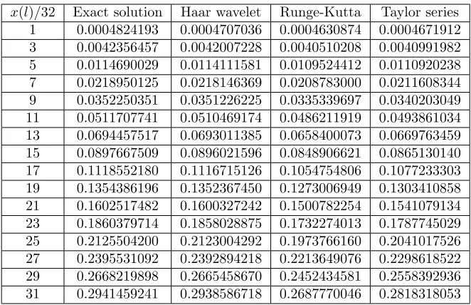
9 Comparison of numerical solutions
Table 1: Results from different numerical methods
x(l)/32 Exact solution Haar wavelet Runge-Kutta Taylor series 1 0.0004824193 0.0004707036 0.0004630874 0.0004671912 3 0.0042356457 0.0042007228 0.0040510208 0.0040991982 5 0.0114690029 0.0114111581 0.0109524412 0.0110920238 7 0.0218950125 0.0218146369 0.0208783000 0.0211608344 9 0.0352250351 0.0351226225 0.0335339697 0.0340203049 11 0.0511707741 0.0510469174 0.0486211919 0.0493861034 13 0.0694457517 0.0693011385 0.0658400073 0.0669763459 15 0.0897667509 0.0896021596 0.0848906621 0.0865130140 17 0.1118552180 0.1116715126 0.1054754806 0.1077233303 19 0.1354386196 0.1352367450 0.1273006949 0.1303410858 21 0.1602517482 0.1600327242 0.1500782254 0.1541079134 23 0.1860379714 0.1858028875 0.1732274013 0.1787745029 25 0.2125504200 0.2123004292 0.1973766160 0.2041017526 27 0.2395531092 0.2392894218 0.2213649076 0.2298618522 29 0.2668219898 0.2665458670 0.2452434581 0.2558392936 31 0.2941459241 0.2938586718 0.2687770046 0.2818318053
10 Conclusion
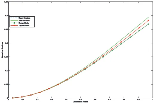
Here, we used three numerical methods to approximate the solutions of damped forced oscillatory differential equation, and compared the results with exact solution. From above results, it is concluded that Haar wavelet method is simple, accurate and more efficient than other well known numer-ical methods for damped forced oscillatory differential equation.
References
1. Babolian, E. and Shahsawaran, A.Numerical solution of non-linear fred-holm integral equations of the second kind using haar wavelets, J. Com-put. Appl. Math. 225 (2009) 87-95.
Table 2: Errors from different numerical methods
x(l)/32 Haar wavelet Runge-Kutta Taylor series 1 0.0000117157 0.0000193319 0.0000152281 3 0.0000349228 0.0001846249 0.0001364475 5 0.0000578447 0.0005165617 0.0003769791 7 0.0000803755 0.0010167125 0.0007341781 9 0.0001024125 0.0016910654 0.0012047302 11 0.0001238567 0.0025495822 0.0017846707 13 0.0001446131 0.0036057444 0.0024694058 15 0.0001645913 0.0048760888 0.0032537369 17 0.0001837053 0.0063797374 0.0041318877 19 0.0002018746 0.0081379247 0.0050975338 21 0.0002190239 0.0101735228 0.0061438348 23 0.0002350839 0.0128105701 0.0072634685 25 0.0002499908 0.0151738040 0.0084486674 27 0.0002636874 0.0181882016 0.0096912570 29 0.0002761227 0.0215785317 0.0109826962 31 0.0002872523 0.0253689195 0.0123141188
3. Chen, C.F. and Hsiao, C.H.Haar wavelet method for solving lumped and distributed-parameter systems, IEEE Proc.: Part D, 144(1) (1997) 87-94.
4. Haar, A. Zur theorie der orthogonalen Funktionsysteme, Math. Annal. 69 (1910) 331-371.
5. Hariharan, G. and Kannan, K.An overview of Haar wavelet method for solving differential and integral equation, World Applied Sciences Journal 23(12) (2013) 1-14.
6. Hsiao, C.H. Wavelet approach to time-varying functional differential equations, Int. J. Computer Math. 87(3) (2008) 528-540.
7. Kouchi, M.R., Khosravi, M. and Bahmani, J. A numerical solution of Homogengous and Inhomogeneous Harmonic Differential equation with Haar wavelet, Int. J. Contemp. Math. Sciences 6(41) (2011) 2009-2018.
8. Lepik, U.¨ Numerical solution of differential equations using Haar wavelets, Math. Comput. Simulat. 68 (2005) 127-143.
9. Lepik, ¨U. Application of Haar wavelet transform to solving integral and differential equation, Proc. Estonian Acad. Sci. Phys. Math. 56(1) (2007) 28-46.
Figure 1: Comparison of graphical solution of different numerical methods.
11. Lepik, ¨U. Haar wavelet method for solving stiff differential equations, Math. Modeling and Analysis 4 (2009) 467-489.
12. Lepik, ¨U.Solution of optimal control problems via Haar wavelets, Int. J. Pure. Appl. Math. 55 (2009) 81-94.
13. Ohkita, M. and Kobayashi, Y.An application of rationalized Haar func-tions to solution of linear differential equafunc-tions, IEEE Trans. Circuit Sys-tem 9 (2003) 853-862.
14. Rama, B.B. and Dukkipati, V.Advanced dynamics, Alpha Science, Pang-bourne, 2001.
15. Razzaghi, M. and Ordokhani,Y.An application of rationalized Haar func-tions for variational problems, Appl. MAth. Comput. 122 (2001) 353-364.
16. Saeed, U. and Rehman, M.U. Haar wavelet operational matrix method for fractional oscillation equations, International Journal of Mathematics and Mathematical Sciences, (2014) 1-8.
17. Simmons, G.F. Differential equations with applications and historical notes, Mcgraw-Hill, London. 1972.
18. Sunmonu, A.Implementation of wavelet solution to second order differen-tial equations with maple, Applied Mathematical Sciences 6(127) (2012) 6311-6326.
رﺎﻫ یﺎﻬﮑﺟﻮﻣ زا هدﺎﻔﺘﺳا ﺎﺑ ﯽﻧﺎﺳﻮﻧ یاﺮﯿﻣ یوﺮﯿﻧ ﻪﻟﺎﺴﻣ یدﺪﻋ ﻞﺣ
رﺎﻣﻮﮐﻮﯿﺷ و ﮏﻨﯿﺳ ﭗﯾرﺪﻨﯾا
نﺎﺘﺳوﺪﻨﻫ ،بﺎﺠﻨﭘ ،رﺎﮐﺪﺒﻣآ ﺮﺘﮐد یروﺎﻨﻓ ﯽﻠﻣ ﻪﺴﺳﻮﻣ
ﯽﻣ ﻪﺋارا ،رﺎﻫ یﺎﻬﮑﺟﻮﻣ زا هدﺎﻔﺘﺳا ﺎﺑ ار ﯽﻧﺎﺳﻮﻧ یاﺮﯿﻣ یوﺮﯿﻧ ﻪﻟﺎﺴﻣ یدﺪﻋ ﻞﺣ ،ﻪﻟﺎﻘﻣ ﻦﯾا رد : هﺪﯿﮑﭼ یﺎﺗﻮﮐ-ﮓﻧار ﺪﻨﻧﺎﻣ ،رﻮﻬﺸﻣ یﺎﻬﺷور زا ﯽﻀﻌﺑ ندﺮﺑ رﺎﮐ ﻪﺑ زا ﻞﺻﺎﺣ ﺞﯾﺎﺘﻧ ﺎﺑ ار ﻞﺻﺎﺣ یدﺪﻋ ﺞﯾﺎﺘﻧ .ﻢﯿﻨﮐ .ﻢﯿﻨﮐ ﯽﻣ ﻪﺴﯾﺎﻘﻣ رﻮﻠﯿﺗ یﺮﺳ یﺎﻬﺷور و ﮏﯿﺳﻼﮐ مرﺎﻬﭼ ﻪﺒﺗﺮﻣ
،ﺖﺳا هﺪﯾدﺮﮔ ﻪﺋارا ﻪﻟﺎﻘﻣ ﻦﯾا رد ﻪﮐ ،رﺎﻫ یﺎﻫ ﮏﺟﻮﻣ زا هدﺎﻔﺘﺳا شور ﻪﮐ ﺪﻨﻫد ﯽﻣ نﺎﺸﻧ یدﺪﻋ ﺞﯾﺎﺘﻧ .ﺪﻨﻫد ﯽﻣ ﺖﺳﺪﺑ ،ﻻﺎﺑ رد هﺪﺷ ﺮﮐذ یﺎﻫ شور ﺎﺑ ﻪﺴﯾﺎﻘﻣ رد ار یﺮﺗ ﻖﯿﻗد ﯽﺒﯾﺮﻘﺗ یﺎﻬﺑاﻮﺟ