Galley
Pro
of
Vol. 8, No. 1, (2018), pp 1–17DOI:10.22067/ijnao.v8i1.60791
A computational method for solving
weakly singular Fredholm integral
equation in reproducing kernel spaces
D. Hamedzadeh and E. Babolian∗
Abstract
In the present paper, we propose a method to solve a class of weakly singular Fredholm integral equations of the second kind in reproducing ker-nel spaces. The Taylor series of the unknown function is used to remove the singularity and bases of reproducing kernel spaces are used to solve this equation. Efficiency of the proposed method is investigated through various examples.
Keywords: Weakly singular kernel; Fredholm integral equations; Taylor se-ries; Reproducing kernel space.
1 Introduction
The Fredholm integral equation with weakly singular kernel arises in differ-ent problems of mathematical physics such as potdiffer-ential problem, variational equilibrium, fracture mechanics, infrared radiation, and elastic contact prob-lems [5,20,21]. Although in [11,16,17,22] authors obtained analytical solution for integral equations with weakly singular kernel in special cases, but gen-erally this is not an easy task. So the numerical analysis standpoint plays major role for solving such equations.
In this paper, we consider Fredholm singular integral equation
∗Corresponding author
Received 5 December 2016; revised 23 March 2017; accepted 14 June 2017 D. Hamedzadeh
Department of Mathematics, Science and Research Branch, Islamic Azad University, Tehran, Iran e-mail: [email protected] and danial [email protected]
E. Babolian
Department of Mathematics, Science And Research Branch, Islamic Azad University, Tehran, Iran e-mail: [email protected]
Galley
Pro
of
µ(x)u(x) +λ(x)
∫ 1 −1
k(x, y)u(y)
(y−x)α dy=f(x), |x|<1 and 0< α≤1, (1)
in which µ(x)̸= 0 and λ(x)= 0, for all̸ x∈ [−1,1], andµ, λ, f, and k are known smooth functions and u is the solution of equation (1) to be deter-mined. We assume that problem has a unique smooth solutionu.Several au-thors considered the numerical solutions of Fredholm integral equations with weakly singular kernel. In [12] Jiang and Cui considered integral equation of first or third kind with weakly singular kernel of the form k(x, y) = Gx(αx,yyβ);
they solved the problem in reproducing kernel spaceW1[0,1].Chen and Zhou
considered second kind Fredholm integral equation with Hilbert type singu-larity [8]. They used transform to remove singusingu-larity and solved problem in W[0,2π] using reproducing kernel method. In [2] Babolian and Arzhang Hajikandi solved (1) with k(x, y) = 1. Du, Zhao, G., and Zhao, C. consid-ered integro-differential equation with logarithmic kernel and Kalman ker-nel with boundary values [10]. They used smooth transform to remove singularity, solving the converted equation with reproducing kernel method in W3[0,1]. Chen and Cheng in [7] used piecewise homotopy perturbation
method (PHPM), for solving integro-differential equation with weakly sin-gular kernel. In [3] authors solved (1), using Taylor series of the unknown function u to remove singularity, and then Taylor expansion of k together with Legendre polynomials as bases to implement Galerkin method. The Sinc-collocation method is studied by Maleknejad, Mollapourasl, and Os-tadi, to solve nonlinear Fredholm integral equations with weakly singular kernel [15]. Beyrami, Lotfi, and Mahdiani solved Fredholm integral equa-tion of the second kind with Cauchy kernel [6]; they removed singularity by smooth transform and used reproducing kernel Hilbert space (RKHS) method to solve problem inW3
o[0,1].Nili and Dastjerdi in [18] solved weakly singular Volterra–Hammerstein integral equation with operational Tau method. We use Taylor series expansion of u(y), at point y = x, to remove singularity; then by use of reproducing kernel spaceWm[−1,1] we convert this equation to a system of linear equations. We demonstrate the method with conver-gence rate O(hm); so when we increase m and move from one reproducing kernel space to other, the rate of convergence will increase.
Galley
Pro
of
2 Preliminaries and notations
In this section we briefly review reproducing kernel properties of the Hilbert spaceWm[a, b] and also fix notations used in this paper. The Hilbert function space,Wm[a, b], is defined as the linear function space
Wm[a, b] ={f|f, f(′), . . . , f(m−1)are absolutely continuous, f(m)∈L2[a, b]},
which is equipped with the following inner product
⟨f, g⟩Wm =
m∑−1
i=0
f(i)(a)g(i)(a) +
∫ b a
f(m)(x)g(m)(x)dx. (2)
The inner product (2) induces the following Hilbert norm
∥f∥Wm =
√
⟨f, f⟩Wm.
The following theorem presents an interesting property of the Hilbert space
Wm[a, b].
Theorem 1. [9]The Hilbert function space Wm[a, b] is a reproducing ker-nel space with the conjugate symmetric reproducing kerker-nel Rm(x, y), that is given by
Rm(x, y) =
lRm(x, y) =∑2i=1mci(y)xi−1, x < y,
rRm(x, y) =∑2i=1m di(y)xi−1, x≥y,
in which coefficientsci(y)anddi(y)are the solutions of the following system of differential equations
(−1)m ∂2mR(x,y)
∂x2m =δ(x−y),
∂iR(a,y)
∂xi −(−1)
m−i−1∂2m−i−1R(a,y)
∂x2m−i−1 = 0,
∂2m−i−1R(b,y)
∂x2m−i−1 = 0, i= 0,1, . . . , m−1,
(3)
whereδ(x−y)is the Dirac delta function.
Remark 1. [9] According to system (3), by use of the Dirac delta function properties, the equation
(−1)m∂
2mR(x, y)
∂x2m =δ(x−y)
Galley
Pro
of
∂i lR m(x,y)
∂xi
x=y
=∂i rRm(x,y)
∂xi
x=y
, i= 0,1, . . . ,2m−2,
∂2m−1lR
m(x,y)
∂x2m−1
x=y+
−∂2m−1 rR
m(x,y)
∂x2m−1
x=y−
= (−1)m.
(4)
By solving the system (4) with boundary condition of (3) with Mathematica, the coefficients ci(y) anddi(y) are computed.
In particular, each functionf ∈Wm[a, b] satisfies the following reproduc-ing property
f(y) =⟨f(.), Rm(., y)⟩Wm ∀y∈[a, b].
Theorem 2.[9]Let R(x, y) be a reproducing kernel ofWm[a, b]; then
∂i+jR(x, y)
∂xi∂yj ∈L
2[a, b], i+j= 2m−1
with respect toxandy and
∂i+jR(x, y)
∂xi∂yj , 0≤i+j≤2m−2,
are absolutely continuous functions in [a, b], with respect to xand y; so we have
∂i+jR(x, y)
∂xi∂yj ∈W
m[a, b], i+j=m−1.
Lemma 1. Let f be a smooth function of order m on [a, b]; then, for k = 1,2, . . . , m, we have f ∈Wk[a, b].
Proof. Let f be a smooth function of order m on [a, b]; thus f(k), for k =
0,1, . . . , m, are continuous functions on [a, b]. Therefore f(k) ∈ L2[a, b], for
k= 1,2, . . . , m, beside the real constants Mk exist which we have
|f(k)(x)| ≤ Mk ∀x∈[a, b];
Galley
Pro
of
3 Removing the singularity and implementation of our
method
Throughout this section, we use the Taylor series to remove singularity of (1); then by use of reproducing kernel space property, we construct our method. With Taylor series of the unknown functionu(y), atx∈[a, b], we have
u(y) =u(x) + (y−x)u′(x) +(y−x)
2
2! u
′′
(x) +· · ·+(y−x) k
k! u
(k)(x)
+(y−x) k+1
(k+ 1)! u
(k+1)(ξ
x,y), (5)
in whichξx,y is betweenxandy.Using (5), thus equation (1) converts to
µ(x)u(x) +λ(x)
(∑k i=0
u(i)(x)
i!
∫ 1 −1
k(x, y)(y−x)i−αdy
+
∫ 1 −1
u(k+1)(ξx,y)
(k+ 1)! k(x, y)(y−x)
k+1−αdy
)
=f(x),
and singularity is removed; now we are in position to define operator L :
Wm[−1,1]→Wm[−1,1],
L(u(.)) =µ(.)u(.) +λ(.)
(∑k i=0
u(i)(.)
i!
∫ 1 −1
k(., y)(y−.)i−αdy
+
∫ 1 −1
u(k+1)(ξ.,y)
(k+ 1)! k(., y)(y−.)
k+1−αdy
)
.
By use of operatorL, the equation (1) is convert to Lu(x) =f(x). It is easy to prove that, for 0≤α <1, operatorLis a bounded linear operator on [−1,1] and that, forα= 1,Lis a bounded linear operator on [−1 +ϵ,1−ϵ] forϵ >0.Let{xi}i∞=1 be a dense subset of interval [a, b], fori= 1,2, . . .; take
y = xi, in Rm(x, y), and define φi(.) = Rm(., xi). Moreover, assume that
ψi=L∗φi, whereL∗ is the adjoint operator ofL.
Theorem 3.Let {xi}∞i=1 be a dense set in [−1,1]; then the functions ψi ∈
Wm[−1,1], and{ψ
i}∞i=1 is complete inWm[−1,1].
Galley
Pro
of
ψi=L∗φi=⟨L∗φi(y), Rm(y, .)⟩Wm
=⟨φi(y), LyRm(y, .)⟩Wm
=⟨φi(y), LyRm(., y)⟩Wm
=⟨LyRm(., y), φi(y)⟩Wm =LyRm(., y)
y=xi
.
Therefore, we get
ψi=µ(xi)Rm(., xi) +λ(xi)
2∑m−1
i=0
1
i!
∂iR m(., s)
∂si
s=xi
∫ 1 −1
k(xi, s)(xi−s)i−αds;
henceψi ∈Wm[−1,1].Letu∈Wm[−1,1], andi∈N. Then we have
⟨u, ψi⟩Wm =⟨u, L∗φi⟩Wm
=⟨Lu, φi⟩Wm
=Lu(xi) = 0.
Since {xi}∞i=1 is dense in [−1,1], we have Lu= 0. By the uniqueness of the
solution of (1), we getu= 0.Hence,{ψi}∞i=1is complete inW
m[−1,1].
As a consequence of Theorem 3, we can expand each function as the following. Let{xi}∞i=1 be dense in [−1,1], and let ube the solution of (1).
Sinceu∈Wm[−1,1], we get
u(x) =
∞
∑
i=0
aiψi(x).
In what follows, we useun as approximate solution of equation (1) which is defined by
um,n(x) = n
∑
i=0
aiψi(x), x∈[−1,1],
and by use of operatorL, we get
n
∑
i=0
ai Lψi(x)≃f(x), (6)
and with inner product of equation (6), withφj, we have
n
∑
i=0
Galley
Pro
of
Thus by replacing ≃ by =, the singular integral problem converts to the linear system of equations Ba = F, in which the coefficient matrix B = [bi,j] = [Lψi(xj)], and the right hand side vector isF = [Fj] =f(xj).4 Error estimate and convergence analysis
In this section first the convergence of the method is investigated, and then the error estimate of proposed method is studied.
Theorem 4.Let{xi}∞i=1 be dense in[−1,1], and let {ψi}∞i=1 be the
orthonor-mal basis ofWm[−1,1]produced by Gram–Schmidt process on{ψi}∞i=1.Then
um,n, the approximate solution of equation (1), and its derivatives are con-vergent uniformly to u; that is, the exact solution of equation (1), and its derivatives, respetively.
Proof. With the Gram process we have
ψi(x) = i
∑
k=1
βikψk(x),
and hence we get
u(x) =
∞ ∑ i=0 i ∑ k=1
aiβikψk(x).
Therefore the approximate solution of equation (1) is
um,n(x) = n ∑ i=0 i ∑ k=1
aiβikψk(x),
and clearly we have limn→∞∥u−um,n∥Wm[−1,1]= 0.On the other hand, we
have
u(x) =⟨u(.), Rm(., x)⟩= m∑−1
i=0
u(i)(1)R(mi)(1, x) +
∫ 1 −1
u(m)(z)R(mm)(z, x)dz.
Differentiating j times with respect tox, we get
u(j)(x) = m∑−1
i=0
u(i)(1)∂ jR(i)
m(1, x)
∂xj +
∫ 1 −1
u(m)(z)∂ jR(m)
m (z, x)
∂xj dz
=⟨u(y),∂
jR m(y, x)
Galley
Pro
of
|u(i)(x)−u(m,ni) (x)|=⟨u(.)−um,n(.),∂
iRm(., x)
∂xi ⟩Wm
≤∥u−um,n∥Wm[−1,1]∥
∂iRm(., x)
∂xi ∥Wm[−1,1].
Since ∂iRm(.,x)
∂xi ∈ Wm[−1,1] and ∥
∂iRm(.,x)
∂xi ∥Wm[−1,1], is continuous with
respect to x, on [−1,1]. For someM >0, we have
∥ ∂iRm(., x)
∂xi ∥Wm[−1,1]≤M, which completes the proof.
Let {xi}ni=1 be a subset of [−1,1], and let −1 < x1 < x2 < · · · <
xn < 1. We define hj := xj+1 −xj, j = 1,2, . . . , n−1, and also put
h:= max1≤j≤n−1hj.
Theorem 5. [4]Let u ∈ Wm[−1,1] be a smooth solution, and let um,n be the approximate solution of the equation (1). Then
∥u−um,n∥∞≤chm,
wherec is a constant.
5 Numerical examples
We examine accuracy and convergence of the proposed method through four examples, which indicate efficiency of the method. The errors were defined as
Em,n=∥u−um,n∥∞≃ max
1≤i≤n|u(xi)−um,n(xi)| m= 1,2, . . . .
Example 1.[3] Consider the following integral equation
u(x) +
∫ 1 −1
(1 +xy+ 2y3)u(y)
(y−x)35
dy=f(x),
wheref is chosen such that
u(x) =x5, x∈[−1,1],
Galley
Pro
of
Table 1: Values ofEm,n, for Example 1.m n= 8 n= 16 n= 32
6 1.72675×10⁻¹ 1.34164×10⁻¹ 1.06141×10⁻¹
8 9.37476×10⁻⁴ 3.09832×10⁻⁴ 2.91592×10⁻⁵
10 6.73973×10⁻⁶ 2.6006×10⁻⁶ 3.41363×10⁻⁶
Table 2: Values ofEm,n, for Example 2.
m n= 8 n= 16 n= 32
4 2.21811×10⁻² 2.89879×10⁻² 7.6194×10⁻²
6 4.92002×10⁻⁴ 7.14302×10⁻⁴ 1.95649×10⁻³
8 2.02376×10⁻⁵ 1.07565×10⁻⁵ 2.91592×10⁻⁵
10 3.13506×10⁻⁶ 1.2141×10⁻⁷ 2.02656×10⁻⁷
shown.
Example 2. Consider the following integral equation
u(x) + (x+ 2)
∫ 1 −1
ex+yu(y)
(y−x) dy=f(x),
wheref is chosen such that
u(x) =xex, x∈[−1,1],
is the exact solution. The numerical results are given in Table 2. In Table 2, for fixedn, by increasingm, the absolute errors converge to zero. In Figures 2, form= 6,8,10, whenn= 8 the approximate solutions and its derivatives have high accuracies.
Example 3.[1, 3, 13, 14]Consider the following integral equation
u(x)−
∫ 1 0
u(y)
|x−y|12
dy=f(x),
wheref is chosen such that
u(x) =x, x∈[0,1]
is the exact solution. For m= 4,6,8, when n= 8, the absolute errors of u
Galley
Pro
of
-0.5 0.0 0.5 1.0
1´10-7
5´10-7
1´10-6
5´10-6
1´10-5
5´10-5
1´10-4
5´10-4
(a) Absolute error foru8(.).
-0.5 0.0 0.5 1.0
5´10-6
1´10-5
5´10-5
1´10-4
5´10-4
0.001 0.005
(b) Absolute error foru(1)8 (.).
-0.5 0.0 0.5 1.0
5´10-5
1´10-4
5´10-4
0.001 0.005 0.010 0.050
(c) Absolute error foru(2)8 (.).
-0.5 0.0 0.5 1.0
5´0.00110-4
0.005 0.010 0.050 0.100 0.500
Galley
Pro
of
-0.5 0.0 0.5 1.0
10-8
10-7
10-6
10-5
10-4
(a) Absolute error foru8(.).
-0.5 0.0 0.5 1.0
10-7
10-6
10-5
10-4
0.001
(b) Absolute error foru(1)8 (.).
-0.5 0.0 0.5 1.0
10-6
10-5
10-4
0.001 0.01
(c) Absolute error foru(2)8 (.).
-0.5 0.0 0.5 1.0
10-6
10-5
10-4
0.001 0.01
Galley
Pro
of
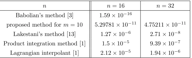
Table 3: The Max Error result of Example 3.n n= 16 n= 32
Babolian’s method [3] 1.59×10⁻¹⁶
proposed method form= 10 5.29781×10⁻¹¹ 4.75211×10⁻¹¹
Lakestani’s method [13] 1.27×10⁻⁶ 2.71×10⁻⁸
Product integration method [1] 1.5×10⁻⁵ 9.39×10⁻⁷
Lagrangian interpolant [1] 2.12×10⁻⁵ 1.94×10⁻⁶
Table 4: The Max Error result ofu(.), Example 4.
m n= 8 n= 16 n= 32
4 3.17985×10⁻⁴ 4.44036×10⁻⁴ 4.24008×10⁻⁴
6 2.38288×10⁻⁶ 2.63628×10⁻⁶ 2.23585×10⁻⁶
8 2.93877×10⁻⁹ 7.58042×10⁻⁹ 3.42293×10⁻⁸
defined as Max Error = max0≤x≤1|u(x)−um,n(x)|.
Example 4.[13, 19]Consider the following integral equation
u(x)− 1 10
∫ 1 0
u(y)
|x−y|13
dy=f(x),
wheref is chosen such that
u(x) =x2(1−x2), x∈[0,1],
is the exact solution. Form= 4,6,8, whenn= 8, the absolute errors ofuand its derivatives are shown in Figures 4. In Tables 4, 5, and 6 the numerical results of proposed method are given. where the Max Error is defined as Max Error = max0≤x≤1|u(i)(x)−u
(i)
m,n(x)|.
Table 5: The Max Error result ofu(1)(.), Example 4.
m n= 8 n= 16 n= 32
4 2.10369×10⁻¹ 7.59437×10⁻³ 7.61556×10⁻²
6 8.89262×10⁻⁶ 2.43063×10⁻⁶ 1.37019×10⁻⁶
Galley
Pro
of
0.2 0.4 0.6 0.8 1.0
10-13
10-12
10-11
10-10
(a) Absolute error foru8(.).
0.2 0.4 0.6 0.8 1.0
5´10-11
1´10-10
2´10-10
51´10-10 ´10-9
2´10-9
5´10-9
(b) Absolute error foru(1)8 (.).
0.2 0.4 0.6 0.8 1.0
10-11
10-10
10-9
10-8
(c) Absolute error foru(2)8 (.).
0.2 0.4 0.6 0.8 1.0
1´10-9
2´10-9
5´10-9
1´10-8
2´10-8
5´10-8
1´10-7
2´10-7
5´10-7
(d) Absolute error foru(3)8 (.). Figure 3: Example 3,m= 4(green line),m= 6(blue dotted),m= 8(red dash).
Table 6: The Max Error result ofu(2)(.), Example 4.
m n= 8 n= 16 n= 32
4 4.6866×10⁻¹ 3.45622×10⁻¹ 3.75916×10⁻¹
6 1.18157×10⁻³ 1.25931×10⁻⁴ 1.20977×10⁻³
Galley
Pro
of
0.2 0.4 0.6 0.8 1.0
51´10-10 ´10-9
5´10-9
1´10-8
5´10-8
1´10-7
5´10-7
(a) Absolute error foru8(.).
0.2 0.4 0.6 0.8 1.0
10-9
10-8
10-7
10-6
10-5
(b) Absolute error foru(1)8 (.).
0.2 0.4 0.6 0.8 1.0
5´10-7
1´10-6
5´10-6
1´10-5
5´10-5
1´10-4
5´10-4
(c) Absolute error foru(2)8 (.).
0.2 0.4 0.6 0.8 1.0
5´10-6
1´10-5
5´10-5
1´10-4
5´10-4
0.001 0.005
Galley
Pro
of
6 Conclusion
Different problems have been solved by researchers using reproducing kernel Hilbert spaces (RKHS). They assume the unknown solution belongs to spe-cial fix W2m and use Gram–Schmidt process to implement RKHS method.
In this paper, we attempted to solve Fredholm integral equations of the sec-ond kind with weakly singular kernel. We used the Taylor series to remove the singularity. According to the problem, we investigated the problem in reproducing kernel spaces Wm[−1,1].In the proposed method by use of re-producing kernel space property, the problem was converted to a system of linear equations. In the proposed method we do not use Gram process, we use RKHS property and use Wm
2 for different m. Though we suppose the
unknown solution is smooth, but this is a very strong assumption, and it is enough for the solution to be in Wm
2 for some m. In this method for fix
m, when the number of basesnincreases the coefficient matrix of the linear system will be ill-conditioned; so we increasemand move from one reproduc-ing kernel to other instead, to find approximate solution with high accuracy. Several test examples were used to show the efficiency and applicability of the method.
Acknowledgements
Authors are grateful to there anonymous referees and editor for their con-structive comments.
References
1. Allouch, C., Sablonn`eire, P., Sbibih, D., and Tahrichi, M.Product integra-tion methods based on discrete spline quasi-interpolants and applicaintegra-tion to weakly singular integral equations, J. Comput. Appl. Math., 233 (2010), no. 11, 2855–2866.
2. Babolian, E. and Arzhang Hajikandi, A. The approximate solution of a class of Fredholm integral equations with a weakly singular kernel, J. Com-put. Appl. Math., 235 (2011), no. 5, 1148–1159.
Galley
Pro
of
4. Babolian, E., Javadi, S., and Moradi, E. Error analysis of reproducing kernel Hilbert space method for solving functional integral equations, J. Comput. Appl. Math., 300 (2016), 300–311.5. Badr, A. A.Integro-differential equation with Cauchy kernel, J. Comput. Appl. Math., 134 (2001), no. 1-2, 191–199.
6. Beyrami, H., Lotfi, T., and Mahdiani, K. A new efficient method with error analysis for solving the second kind Fredholm integral equation with Cauchy kernel, J. Comput. Appl. Math., 300 (2016), 385–399.
7. Chen, Z. and Cheng, X. An efficient algorithm for solving Fredholm integro-differential equations with weakly singular kernels, J. Comput. Appl. Math., 257 (2014), 57–64.
8. Chen, Z. and Zhou, Y.An efficient algorithm for solving Hilbert type singu-lar integral equations of the second kind, Comput. Math. Appl., 58 (2009), no. 4, 632–640.
9. Cui, M. and Lin, Y.Nonlinear numerical analysis in the reproducing kernel space, Nova Science Publishers, Inc., New York, 2009.
10. Du, H., Zhao, G., and Zhao, C. Reproducing kernel method for solving Fredholm integro-differential equations with weakly singularity, J. Comput. Appl. Math., 255 (2014), 122–132.
11. Estrada, R. and Kanwal, Ram P.Singular Integral Equations, Birkh¨auser Boston, Inc., Boston, MA, 2000.
12. Jiang, W. and Cui, M.The exact solution and stability analysis for in-tegral equation of third or first kind with singular kernel, Appl. Math. Comput., 202 (2008), no. 2, 666–674.
13. Lakestani, M., Nemati Saray, B., and Dehghan, M. Numerical solution for the weakly singular Fredholm integro-differential equations using Legen-dre multiwavelets, J. Comput. Appl. Math., 235 (2011), no. 11, 3291–3303.
14. Long, G., Nelakanti, G., and Zhang, X.,Iterated fast multiscale Galerkin methods for Fredholm integral equations of second kind with weakly singu-lar kernel, Appl. Numer. Math., 62 (2012), no. 3, 201–211.
15. Maleknejad, K., Mollapourasl, R., and Ostadi, A.Convergence analysis of Sinc-collocation methods for nonlinear Fredholm integral equations with weakly singular kernel, J. Comput. Appl. Math., 278 (2015), 1–11.
Galley
Pro
of
17. Muskhelishvili, N. I. Singular Integral Equations. Boundary problems of function theory and their application to mathematical physics, Translation by J. R. M. Radok. P. Noordhoff N. V., Groningen, Holland, 1953.18. Nili Ahmadabadi, M. and Laeli Dastjerdi, H.Tau approximation method for the weakly singular Volterra-Hammerstein integral equations, Appl. Math. Comput., 285 (2016), 241–247.
19. Okayama, T., Matsuo, T., and Sugihara, M.Sinc-Collocation methods for weakly singular Fredholm integral equations of the second kind, J. Comput. Appl. Math., 234 (2010), no. 4, 1211–1227.
20. Schneider, C.Product integration for weakly singular integral equations, Math. Comp., 36 (1981), no. 153, 207–213.
21. Schneider, C.Regularity of the solution to a class of weakly singular Fred-holm integral equations of the second kind, Integral Equations Operator Theory, 2 (1979), no. 1, 62–68.
Ĉ̒˵͍̔̒̔ ͋˵̫̾͐î Ċ ĉöîù̦͏̡̒ Ć̒˵͒îö
˳̴̒˴ø ĉĊ̨˛ áĈį͖̘̂ ñ͇̒˵̢͇̘ Ċ ć͍͗̽ ̡̦îĊ á˳͏̫ͣî öîùé ĉ̒˜̯͒îö
ĝğĥŞ öîǫ̤̈ ĞŜ ͔͇͌̒͏ ų̂˴̧ˉ áĝğĥŞ ͑˴öøĊ̨̓ ğ ĉ̦̮ ô̱ͣî ͔͇͌̒͏ ̗̓̒˴øö áĝğĥŝ ø÷é ĝŝ ͔͇͌̒͏ ̗̓̒˴øö
ǫ͓̈̈́͏ ͔̙̬͕ ̒̔ ćĊö Ā͗͒ ͎͍͕ǫ̈̓ Ćį̂˜̙͒î ñ͢ö̒̾͏ ùî œî ͔̙̫ö ̡͋ œį̂̔ ̦˴̦̞ ˳̮Ċø á͔͇͌̒͏ ͑˴î øö ĉ̦˵˙˒
͔͌ö̒̾͏ ˳˜͓˵˙̘ Ć͖̟͗͏ ̼̘̔̒ ø͍͗˵̘ ̶̬̔ ùî ĉö̙̫̒̈́î ̒̔ ͎˵͓˙˵͏ ˳̨̓̾͏ ̦˵̘͌͗ù̒̔ ͔̙̬͕ œ̵͕̒̒̓ øö îø ͂˵̴̾ ̦͓˒ ̒̔ ̗˴͖̒͒ øö ͎˵͓˙˵͏ ̡͋ îø ͔͌ö̒̾͏ ̦˵̘͌͗ù̒̔ ͔̙̬͕ œ̵͕̒̒̓ ͔˴̒ˉ ùî ĉö̙̫̒̈́î ̒̔ ͔͏îöî øö Ċ ĉǫ̈˘ ̼̓ø îø ͎˵͕̦˵͏ Ĉ̯̒͒ îø ýĊ̨̈́͏ ûĊø ˳˴îø̒˘ œö̦̽ Ć̜̒͏