Valuation of American Options

(1)

Valuation of American Options

Dr. Christian Hoffmann

Department for Continuing Education

University of Oxford

A thesis submitted for the degree of

Diploma in Mathematical Finance

(2)

The valuation of American options is a difficult problem. The basic reason is that the asset price at which early exercise is optimal isn’t known in advance and has to be found as part of the solution of the problem. In mathematical terms, a partial differential

equation known as Black–Scholes equation has to be solved with a moving boundary condition. This is known in general as amoving boundary problem. Analytic solutions of this kind of problems can be found only in very special cases (e.g. for the American call on an asset paying a single discrete dividend during the lifetime of the option).

However, because of the practical importance of American options, their efficient and accurate pricing is vital for option market participants. Finite difference methods can be used to solve the differential equation numerically, but in order to obtain an accurate solution, considerable computational effort is necessary. Therefore other, more efficient methods have been developed.

In this thesis a comparison of numerical and approximative methods to solve this

(3)

List of Figures

2.1 Binomial model with a single time step . . . 8

2.2 Binomial tree with 3 time steps . . . 10

2.3 Price of an American call option with binomial trees . . . 13

3.1 Non-linear transform of S . . . . 16

4.1 Comparison of the call prices with the finite difference solution . . . 26

4.2 Comparison of the put prices with the finite difference solution . . . 28

4.3 Distribution of deviations for American calls on FX rates rates . . . 29

4.4 Distribution of deviations for American puts on FX rates . . . 31

(6)

3.1 Optimisation of the grid for European and American calls . . . 21

3.2 Parameters for validation scan . . . 22

3.3 Deviation of the finite difference solution from the analytical solution. . . 23

4.1 Parameters for comparison of methods . . . 24

4.2 Parameter domains . . . 25

4.3 Statistical data for calls on equity . . . 27

4.4 Statistical data for puts on equity . . . 27

4.5 Statistical data for the call on an FX rate . . . 30

4.6 Statistical data for the put on an FX rate . . . 32

4.7 Problematic regions of the different methods . . . 33

(7)

Chapter 1

Introduction

A (so called plain vanilla) financial option gives the holder the right to buy or sell the underlying asset for astrike or exercise price X (that is fixed when the option is written) at a later time. If the holder has the right to buy the asset, the option is acall, while a put gives the holder the right to sell the asset. The use of this right by the holder is calledexercise of the option. The option is calledEuropean if it can be exercised only at a certain date (the expiration or maturity date T ). An American option can be exercised at any time before the expiration date. If an American option is

exercised before the expiration date, it isearly exercised.

Becaue the option gives the holder theright, but not the obligation to buy or sell the asset, he will only exercise the option if it is profitable for him, i.e. he will only exercise a call if the market price of the asset is above the strike price or he will only exercise a put if the market price of the

asset is below the market price. The option provides its holder with the possibility of unlimited profit at the risk of a limited loss. Therefore it has a value. Acquiring an option costs apremium.

The value of the option at expiry is thepayoff of the option. It is zero if exercising the option doesn’t provide a profit and positive otherwise. For plain vanilla options it can be written as

Pcall(S) = max(0;S X) (1.1a)

Pput(S) = max(0;X S): (1.1b)

At any time before expiry, the value of the option will be different from the payoff. For a European option it will be the expectation value of the payoff at expiry discounted to the date the valuation is done for (given the interest rate, the price and the volatility of the underlying asset).

Because an American option can be exercised at any time, its value can never be less than the payoff. (Otherwise, it would be exercised immediately.) Furthermore, because the early exercise is an additional right to the exercise at expiry, an American option is at least as valuable as a European option. The exact determination of the value of the American option, however, is in general a difficult task. Analytic closed–form solutions can be found only in rare special cases. A numerical

solution of this problem can be found (in principle) with arbitrary accuracy limited only by the properties of the numerical scheme, but involving a significant computational effort.

Most of the options traded at exchanges are American. Therefore, an accurate and efficient valuation of American options ist very important. Thus other ways must be found to find the option

(8)

(9)

Chapter 2

Foundations

2.1 Pricing of Financial Derivatives

In this chapter the notation used in the following chapters shall be introduced. The derivation of

the differential equation which is the basis of the discussion in the later chapters is outlined. The purpose of this chapter is not a rigorous mathematical treatment of stochastic calculus. A good introduction can be found e.g. in [1].

2.1.1 Wiener Processes

If the value of a variable changes over time in an uncertain way it is said to follow astochastic process. This process can be discrete or continuous in time (discrete time or continuous time pro-cess) and in “space” (discrete or continuous variable). Although trading in financial markets isn’t

continuous in time (there is no trading outside business hours at exchanges) and asset price (e.g. stock prices are quoted in fixed ticks), the continuous-time, continuous-variable process is a useful model of financial asset prices for many purposes.

AMarkov process is a stochastic process where only the present value of a stochastic variable is relevant for the next value. The next value is independent of the path the present value is obtained. A Wiener process is a particular Markov process with a mean change of 0 and variance 1. In physics

the process is often referred to as Brownian motion. If a random variable X follows a Wiener process, its changes∆X in discrete time steps∆t can be written as

∆X=ε p

∆t (2.1)

whereεis a random drawing from a standardised normal distribution1. In the limit∆t!0 this can

formally be written as

dX =ε p

dt (2.2)

If the development of a stochastic variable S with time t can be described as ageneralised Wiener process, its differential equation can be written as

dS=Mdt+ΣdX (2.3)

1_{A normal distribution with mean 0 and variance 1}

(10)

where the parameters M andΣare constant. M describes the drift of the process, andΣis a measure of its variation. The differential dX is a random variable drawn from a normal distribution with mean 0 and variance dt (i.e. a Wiener process as in equation 2.2). The values of dX for different times are independent.

The prices of financial assets are usually assumed to follow more general processes where the parameters can depend on S and t.

dS=M(S;t)dt+Σ(S;t)dX (2.4)

These processes are calledItˆo processes. For many financial assets (e.g. equities, FX rates) a log-normal random walk2of the asset price is assumed. In this case M(S;t)=µS andΣ(S;t)=σS where

σand µ are constant. Equation 2.4 then can be written as

dS=µSdt+σSdX: (2.5)

The parameterσis calledvolatility, µ is called drift.

2.1.2 Risk-neutral Valuation

A world in which investors don’t require a compensation for risk is called risk-neutral. In such a

world the expected return on any security is the risk-free rate. The Girsanov theorem can be used to transform the random walk with drift µ in equation 2.5 to the risk–neutral random walk

dS=rSdt+σSdX: (2.6)

where the drift is equal to the risk–free rate r. If the asset pays a continuous dividend yield q, the growth rate of the asset price has to be reduced by this amount in order to provide the same overall

return (dividend + capital gain) as an asset without dividends:

dS=(r q)Sdt+σSdX: (2.7)

The following derivation will be based on this random walk.

2.1.3 Itˆo’s Lemma

Suppose a function V(Xt;t)is given where the subscript t indicates that X is itself a function of time.

In “normal”3calculus there is the chain rule how to calculate thetotal derivative of V with respect to t:

dV dt =

∂V

∂X

dX dt +

∂V

∂t: (2.8)

An equivalent formulation in terms of the differential is

dV =

∂V

∂XdX+

∂V

∂tdt: (2.9)

(11)

2.1. PRICING OF FINANCIAL DERIVATIVES 5

Itˆo’s lemma is the equivalent if the variable Xt is a stochastic variable following a Wiener process at time t. Using a Taylor expansion of V to order dt neglecting all terms of higher order as dt!0, we

obtain

dV =

∂V

∂tdt+

∂V

∂XdX+

1 2

∂2_V

∂X2dX 2

=

∂V

∂t +

1 2

∂2_V

∂X2

dt+

∂V

∂XdX (2.10)

because the increment dX is drawn from a normal distribution with variance dt (implied by the fact that X follows a Wiener process) and therefore dX2 is of the order of dt. If V is contingent on a variable S following an Itˆo process 2.4, this can be generalised to

dV =

M(S;t)

∂V

∂t +

1 2Σ(S;t)

2∂2V

∂S2

dt+

∂V

∂SdS (2.11)

An application of Itˆo’s lemma that will later be useful is to consider the process in equation 2.7 and V(S)=ln S. Then

dV =

∂V

∂SdS+

1 2σ

2_S2∂2V

∂S2dt

=

1

S((r q)Sdt+σSdX)

1 2σ

2_S21

S2dt

=

r q σ

2

dt+σdX

d ln S=

r q σ

2

dt+σdX (2.12)

The random variable ln S follows a normal generalised Wiener process4, but the drift has an addi-tional volatility–dependent component.

2.1.4 Derivation of the Black Scholes Equation

The following assumptions have to be made for the derivation:

The asset price is a continuous variable that can change continuously in time and follows a

random walk as in equation 2.7.

Short selling of securities is permitted (with full use of the proceeds).

There are no transaction costs, bid-ask spreads, or tax considerations.

It is possible to adjust a portfolio continuously in time and asset quantity (i.e. the asset is

perfectly divisible).

The asset doesn’t pay discrete dividends during the lifetime of the derivative.

(12)

There is no arbitrage possibility.

Borrowing and lending at the risk-free rate is possible.

The risk-free rate is constant in time and independent of the maturity (i.e. the rate curve is

flat).5

The liquidity of the market is unlimited.

There is no counterparty/default risk.

Let S be the price of an asset with dividend yield q. Let V(S;t)be the price of a derivative on

this asset. The change of the derivative value can be expressed using Itˆo’s lemma 2.11 and based on the random walk in equation 2.7 as

dV =

∂V

∂t dt+

∂V

∂SdS+

1 2σ

2_S2∂2V

∂S2dt (2.13)

A hedged portfolio with valueΠis constructed containing the option on one unit of the asset and the fraction ∆of the asset itself:

Π=V ∆S (2.14)

In an infinitesimal time step dt, the value of the portfolio changes by dΠ. The asset value changes by the (random) increment dS. Using equation 2.13 and assuming that ∆is constant during dt we obtain utilising Itˆo’s lemma (equation 2.11)

dΠ=dV ∆dS

=

∂V

∂tdt+

∂V

∂SdS+

1 2σ

2_S2∂2V

∂S2dt ∆dS:

The portfolio is risk-free if dΠis independent of dS. This is accomplished by letting∆=

∂V ∂S. Then the return on the portfolio reduced by the dividend the portfolio holder has to pay on the asset he is short should be equal to the risk-free rate.

dΠ qS∂V

∂Sdt=

∂V

∂t +

1 2σ

2_S2∂2V

∂S2 qS

∂V

∂S

dt

=rΠdt =r(V ∆S)dt =r

V ∂V

∂SS

dt

Rearranging this result yields the Black-Scholes equation

∂V

∂t +

1 2σ

2_S2∂2V

∂S2 +(r q)S

∂V

∂S rV =0: (2.15)

(13)

2.2. SOLUTION OF THE BLACK SCHOLES EQUATION FOR EUROPEAN OPTIONS 7

The payoff at maturity determines the option price at any time prior to expiry. For vanilla options

as described in chapter 1 it can be written as

Pcall(S)=max(0;S X) (2.16a)

Pput(S)=max(0;X S): (2.16b)

Thus, the value of the option is known at expiry. Let t be the instant of time at which the fair option

price V(S;t) is to be determined. This option price is the solution of the Black-Scholes equation.

The Black-Scholes equation is a parabolic equation that can be solved only for decreasing t. The

payoff is a ”final condition”. Usingτ=T t as the time variable, the Black-Scholes equation can

be solved as an initial value problem with the option payoff as the initial condition.

2.2 Solution of the Black Scholes Equation for European Options

2.2.1 Analytic solution

For European options, the Black-Scholes equation can be solved analytically by transforming it to

the heat equation. The algebra of this solution can be found e.g. in [4]. In the original Black-Scholes

equation the dividend yield q=0, but conceptually this doesn’t make any difference. Therefore here

only the more general case is considered here.

2.2.1.1 Option on an Asset with a Continuous Dividend Yield

This case is valid for options on equity indices with a continuous dividend yield q, futures with

q=r, FX rates with q=rf (where rf is the foreign interest rate) and assets without dividends

(q=0).

The price of a European Call is

Vcall=e

q(T t)

SN(d1) e

r(T t)

X N(d2) (2.17)

with

d1=

ln(S=X)+(r q+σ

2

=2)(T t)

σp

T t (2.18a)

d2=d1 σ p

T t: (2.18b)

N(x)is the cumulative normal distribution as defined in equation D.1. The price of a European put

is

Vput=e

r(T t)

X N( d2) e

q(T t)

(14)

uS

dS 1-p

[image:14.612.235.320.57.161.2]

p S

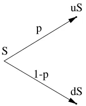
Figure 2.1: Binomial model with a single time step

2.2.1.2 Option on Equity with Discrete Dividends

If the asset underlying the options pays discrete dividends (known in advance), the process govern-ing the asset price S can be divided in a deterministic part D (the present value of all future dividends falling into the lifetime of the option) and a stochastic process followed by S0

according to

dS0 =rS

0

dt+σ 0

S0

dX (2.20)

The asset price is then S=S 0

+D The volatility of the modified process has in principle to be scaled

from the volatility of the process followed by S toσ0

=σ

S

S D. However for sake of simplicity in all examples with discrete dividends it is assumed that the volatility of S0

is given as σinstead of the volatility of S.

2.2.2 Numerical Solution of the Black-Scholes Equation

Because the Black-Scholes equation 2.15 is a parabolic equation, it can be solved by the usual

implicit or explicit finite difference methods [12]. A Crank-Nicolson scheme has been used that is described in chapter 3. The numerical solution has the advantage over the analytic solution that it is applicable to a much greater variety of options. For European options the analytic solution can be used to assess the accuracy of the numerical solution.

2.2.3 Binomial Trees

The idea of the binomial tree is a simplified model of asset prices: after one time step δ, the asset with price S at time t can only take one of two different values uS and dS with probability p and 1 p, respectively, at time t+δ (see figure 2.1). The drift and the volatility of the continuous

process has to be matched by adjusting u, d and p. The valuation is done in a risk-neutral world,

i.e. the drift is r.6 The expected value of S at time t+δgiven S(t)is then (with E[XjY]denoting the

expected value of X given Y )

E[S(t+δ)jS(t)]=pS(t)u+(1 p)S(t)d =e

(r q)δ

S(t) (2.21a)

6_{Therefore the probability p is a risk-neutral probability. It must not be confused with the “true” probability in the}

(15)

2.2. SOLUTION OF THE BLACK SCHOLES EQUATION FOR EUROPEAN OPTIONS 9

Having defined ˆSδ_t =E[S(t+δ)jS(t)], the variance of S is

E[(S(t+δ) Sˆ

δ

t)

2

jS(t)]=E[S(t+δ)

2

jS(t)] Sˆ

δ2

t

=pS(t)

2_u2

+(1 p)S(T)

2_d2

(pS(t)u+(1 p)S(t)d)

2

=S(t)

2_σ2_δ _(2.21b)

The two equations 2.21a and 2.21b can be simplified to obtain

e(r q)δ

=pu+(1 p)d (2.22a)

σ2_δ

=pu

2

+(1 p)d

2

(pu+(1 p)d)

2

(2.22b)

One degree of freedom remains, leaving us with a choice. The choice made here is u=1=d as

proposed by Cox, Ross and Rubinstein [2]. The solution of the nonlinear equations for u, d and p

can be approximated using the Taylor expansion of the exponential function to first order inδ. The result is

u=e

σp

δ _(2.23a)

d=e

σp

δ _(2.23b)

p= e(r q)δ

d

u d

: (2.23c)

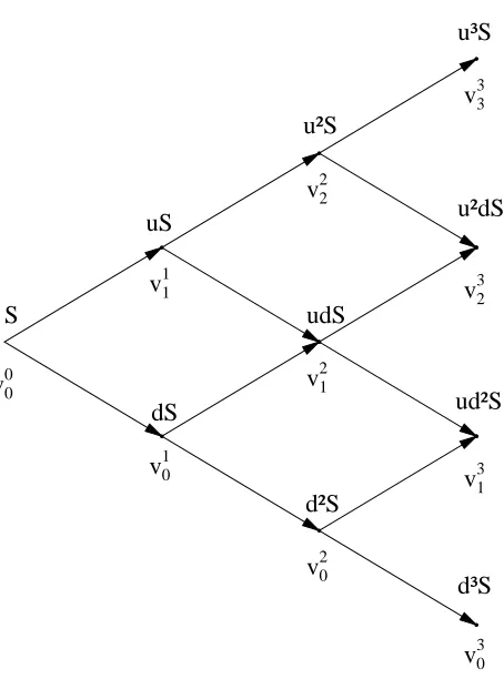
This model is too simple to be realistic with only one time step. Generally the time to expiry T of an option is chopped into a number M of time steps such thatδ=T=M. For 3 time steps we get

for the evolution of asset prices the picture in figure 2.2. In every time step k the nodes of the tree

represent asset prices S_ik=Su

i_dk i_{. The tree of asset prices is built using u and d until the expiry}

date of the option. Then the option price vM_i for every asset price SM_i is calculated at expiry as the

payoff. Going back through the tree, the option price is calculated as

vk 1_i =e

rδ

pvk_i+1

+(1 p)v

k i

: (2.24)

Since p is interpreted as a probability, the condition 0p1 must be satisfied. This imposes

a stability condition of the method:

δ<

σ2

(r q)

2 (2.25)

Ifδand therefore also the size of the step in the asset price is small enough, the continuous process can be modeled accurately. The stability condition 2.25 has to be obeyed.

2.2.4 Treatment of Discrete Dividends with Binomial Trees

If discrete dividends are payed during the lifetime of the option, an adjusted process is used accord-ing to equation 2.20 is used. Therefore the picture in figure 2.2 refers then to the process S0

(16)

v0₀

S udS

u²dS

d³S ud²S u²S

d²S dS

uS

u³S

1 1

1

v2₀

v3 v3₁ v2₁

v3₂ v₂

v3

v₀ v

2

3

[image:16.612.164.391.96.402.2]

0

Figure 2.2: Binomial tree with 3 time steps

and added to the asset prices during the time step. Therefore if a single dividend D is payed at time τwith 0<τ<T , the real stock price at node(i;k)is

S_ik=S 0k

i +Θ(τ kδ)De

r(τ kδ)

(2.26)

whereΘ(:)is the Heaviside-function which is 1 when its argument is greater than 0 and zero

else-where. This formula can be generalised easily to assets with more than one dividend.

2.3 American Options

For American options a solution of the Black Scholes equation in general can’t be found analytically. The reason is that the point at which early exercise of the option at any instant of time is optimal is a priori unknown. In the framework of the PDE it can be treated as a free boundary problem.

The equality in equation 2.15 becomes an inequality: For the Delta–hedged portfolioΠthe change in value over time dt is dΠ. Arbitrage consideration show that it is impossible to have dΠ>rΠdt

(17)

2.3. AMERICAN OPTIONS 11

earn the risk–free rate on the money) is not always possible in the presence of early exercise. While

in the case of a European option the return on the option in a risk-neutral world must be equal to the

risk-free rate, in the case of the American option the following inequality holds:

dΠ=

∂V

∂tdt +

1 2σ

2_S2∂2V

∂S2dt

rΠdt =r(V

∂V

∂SS )dt

,

∂V

∂t +

1 2σ

2_S2∂2V

∂S2 +(r q)S

∂V

∂S rV0: (2.27)

An additional condition is that the option value is always greater or equal to the payoff p(S)

Vp(S): (2.28)

If the situation V<p(S) occured, the option would be exercised immediately, and its payoff (and

therfore also its value) would be p(S). If the option value V >p then early exercise doesn’t occur,

and therefore the portfolio can be shorted. Defining the operator

L

=

∂ ∂t

+

1 2σ

2_S2 ∂2

∂S2+(r q)S

∂ ∂S r

; (2.29)

in this case

L

V =0 must be satisfied. If

L

V<0, the option should be exercised early, and therefore

V=p. This can be formulated as thelinear complementarity problem:

L

V 0 (2.30a)

V p(S)0 (2.30b)

(V p(S))

L

V =0 (2.30c)

For American calls on an asset without dividends it can be shown that early exercise is never

optimal because the option value is always higher than the payoff. In this special case the value of

the American option is equal to the value of the equivalent European option. If the asset pays

dis-crete dividends, early exercise of a call can be optimal only immediately before a dividend payment

in order to cash in the dividend. If there is only one dividend payment during the lifetime of the

option, an analytic solution does exist.

2.3.1 Analytic Solution for American Calls with one Discrete Dividend

For the case that the asset pays exactly one known discrete dividend during the lifetime of the option,

(18)

and Whaley [6, 7, 8]. This is possible because early exercise is optimal only at one instance of time

(namely at the dividend payment date). With the dividend D at time t0

the solution is

Vcall=

S De r(t 0

t)

N(b1)+M a1; b1; r

t0 t

T t

!!

X e r(T t)

M a2; b2; r

t0 t

T t

!

(X D)e

r(t

0

t)

N(b2) (2.31a)

where

a1=

lnS Der(t 0

t)

X +(r+σ

2

=2)(T t)

σp

T t (2.31b)

a2=a1 σ p

T t (2.31c)

b1=

lnS Der(t 0

t)

I +(r+σ

2

=2)(t 0

t)

σp t0

t (2.31d)

b2=b1 σ p

t0 t

; (2.31e)

N(x)is the cumulative normal distribution as defined in equation D.1, and M(x;y;ρ)is the

cumula-tive bivariate normal distribution as defined in equation D.4. The variable I is the critical ex-dividend stock price I that solves

V_callBS(I;X;T t 0

)=I+D X (2.32)

where V_callBSis the value of a European call with stock price I and time to maturity T t0

. If D X(1 e

r(T t

0 )

)or I=∞, it won’t be optimal to exercise the option early. The price of the option is

then equal to the price of the equivalent European option.

2.3.2 Numerical Solution

The linear complementarity problem can be solved numerically in principal with arbitrary accuracy limited only by computation time, machine accuracy, and the stability of the numerical scheme.

The details of the Crank-Nicolson scheme used for the work presented in this thesis are described

in chapter 3.

Because the numerical solution is (in principle) exact, it can be used as a benchmark for other

(faster) methods approximating the solution of the Black-Scholes equation.

2.3.3 Binomial Tree

The binomial tree can be used almost unchanged to value American option. Only equation 2.24 has

to be modified in the following way:

vk 1_i =e

rδ_max

pvk_i+1

+(1 p)v

k

i;P(S

k 1

i )

(19)

2.3. AMERICAN OPTIONS 13

Number of steps

option value

1.15 1.16 1.17 1.18 1.19

15 16 17 18 19 20 ₁₀₀ ₁₀₁ ₁₀₂ ₁₀₃ ₁₀₄ ₁₀₅ ₂₀₀ ₂₀₁ ₂₀₂ ₂₀₃ ₂₀₄ ₂₀₅ ₃₀₀ ₃₀₁ ₃₀₂ ₃₀₃ ₃₀₄ ₃₀₅ ₅₀₀ ₅₀₁ ₅₀₂ ₅₀₃ ₅₀₄ ₅₀₅

[image:19.612.100.518.62.299.2]

1000 1001 1002 1003 1004 1005

Figure 2.3: Price of an American call option with one dividend calculated with binomial trees with

different numbers of time steps (solid line). The dashed line indicates the true price calculated with the formula of Roll, Geske and Whaley. The parameters are S=X=100, r=0:04,σ=0:4, D=4, the time to maturity is 0.915 years and the time to the ex–dividend date is 0.61 years.

where P(S)is the payoff of the option at the asset price S. Figure 2.3 shows how the price of an

American call option on an asset paying one discrete dividend varies with the number of steps in

the binomial tree. The price oscillates about the true price (indicated by the horizontal dashed line)

calculated with the analytic formula of section 2.3.1. The amplitude of these oscillations decays

only very slowly.

A better option price can generally by obtained by calculating it with two binomial trees with

step numbers N and N+1 and taking the average. In some cases this average is close to the true

option value.

2.3.4 Control Variate Technique

The error of the binomial tree can be reduced by using it only to calculate the difference between

the price of the American and the equivalent European option with the same strike and the same

time to maturity. The analytical solution of the Black-Scholes equation for European option is

then corrected with this difference, or in other words, the price of the European option is used as

a control variate for the price of the American option. Letting ve the Black-Scholes price of the

European option, vE the price of the European option calculated with the binomial tree, vAthe price

(20)

vais

va=ve+vA vE (2.34)

2.3.5 Analytic Approximations

There are two important analytic approximations for the value of American options without discrete

dividends [5]. They both allow for a continuous dividend yield q. If q0, early exercise of an

American call is never optimal, and its value is equal to the value of a European call.

One of these approximations has been developed by Barone-Adesi and Whaley [9]. The formula is shown in appendix A.1. The other later developed formula of Bjerksund and Stensland [10] is

(21)

Chapter 3

The Finite Difference Scheme

The differential equation to be solved is the Black Scholes equation

∂V

∂t +

1 2σ

2_S2∂2V

∂S2 +(r q)S

∂V

∂S rV=0 (3.1)

The coefficientsσ, r and q are assumed to be constant. The Black–Scholes equation is a parabolic equation, similar to the heat or diffusion equation ∂_∂u_t =

∂ ∂x

D∂_∂u_x

.1 Thus it falls in the category of the initial value problems which describe the evolution of an initial state with time. For the

numerical solution an important issue is the choice of astable method (opposed to boundary value problems where efficiency is the greater issue).

Various methods are discussed in reference [12]. For this kind of problems one could generally

choose any simple explicit or implicit method. While the implicit scheme is unconditionally stable, for the explicit scheme the size of the grid in “space” and time must be made small enough to obtain

a numerically stable result. Both methods have a local truncation error of the order O(δt). For

the purpose of this project, the finite difference scheme used is the Crank–Nicolson scheme. It is

basically a combination of an implicit and an explicit scheme that effectively calculates a central

derivative in time for points in the middle of two time grid points. The local truncation error is of the order of O(δt

2

). At the boundaries S=0 and S=∞, the second derivative

∂2_V

∂S2 is set to 0.

The finite difference scheme should operate on an equally spaced grid in order to keep the convergence properties. However the error is not only dependent on the grid spacingδS, but also on

the second derivative∂_∂2_SV2. To improve the overall error without increasing the computational effort

it would make sense to make the grid finer where the second derivative is large, i.e. where the asset

price is close to the strike price. Both goals can be accomplished by transforming the asset price

with a non–linear invertible function to the new variable

˜

s=asinh(S k) asinh( k) (3.2)

(based on an idea from [11]) and using a homogeneous grid in ˜s. The grid in S is then compressed

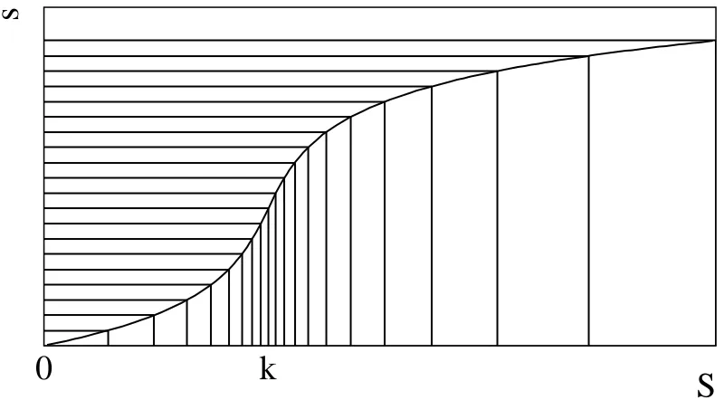
near S=k and stretched if S is far away from k (see figure 3.1). For the purpose of this calculation,

1_{Actually by some variable transforms, the Black–Scholes equation can be reduced to the heat equation.}

(22)

S

s˜

[image:22.612.81.481.61.282.2]

0 k

Figure 3.1: Non-linear transform of S (equation 3.2). It can be seen how a constant spacing in ˜s leads to a compression of the grid in S about k and a stretching at large S.

k is set equal to the strike X . The Black Scholes equation 3.1 can be written in terms of this new

variable as

∂V

∂t +

1 2σ

2_T

(s 0

)

2∂2V

∂s˜2 +

r q 1

2σ

2_T

(s 0

)tanh s 0

| {z }

=: f(s 0 )

T(s 0

)

∂V

∂s˜ rV=0 (3.3)

with the definitions

c=asinh( k) (3.4a)

s0

=s˜+c (3.4b)

T(x)=

sinh x+k

cosh x (3.4c)

3.1 Discretisation

The function V is mapped to a grid in “space” S2and time t. The number N of steps in S determines together with the lower boundary Smin and the upper boundary Smax the size of a step in S δS= (Smax Smin)=N, and the number M of time steps determines with the lifetime T of the option to be

valued the size of a time stepδt=T=M. The values Si=Smin+iδS with 0iN mark the grid

points in S, the values tk

=kδt with 0kM mark the time steps. The function values on the grid

are V_ik where i represents the space dimension and k represents the time dimension. The following

(23)

3.1. DISCRETISATION 17

discrete approximations for the partial derivatives of V are used:

∂V

∂t =

Vk+1

i Vik

δt

+O(δt) (3.5a)

∂V

∂S =

V_ik +1

V_{i 1}k

2δS

+O(δS

2

) (3.5b)

∂2_V

∂S2 = V_ik

+1

2V_ik+V

k i 1

δS2 +O(δS

2

): (3.5c)

The discretisation of equation 3.3 with the Crank Nicolson scheme yields

Vk+1

i Vik

δt +

1 2σ 2_T (s 0 i)

2Vik+1

2V_ik+V

k

i 1+V

k+1

i+1

2Vk+1

i +V

k+1

i 1 2δs˜2

+f(s 0

i)T(s

0

i)

V_ik +1

V_{i 1}k +V

k+1

i+1

Vk+1

i 1 4δs˜

r

2(V

k

i +V

k+1

i )=0 (3.6)

with a local truncation error of the order O(δt

2

;δs˜

2

) Collecting the terms, multiplying by δt and

rearranging the equation to have all variables of a time step on the same side one gets for the points inside the grid(0<i<N)

AiVk

+1

i 1 +(1+Bi)V

k+1

i +CiV

k+1

i+1

= AiV

k

i 1+(1 Bi)V

k

i CiVik+1 (3.7)

The coefficients Ai, Biand Ciare independent of the time step k because the coefficients of equation

3.1 are constant in time. Their definition can be found as equation B.2 in appendix B.1.

The method is well–suited for diffusion equations. If, however, the coefficient of∂_∂V_S is very large compared to the coefficient of∂_∂2_SV2, the equation describes more a transport than a diffusion

problem, and the discretisation scheme will not find the right solution because the central difference for ∂_∂V_S can’t describe the flow of information correctly. Therefore the condition

1 2σ 2_T (s 0 )

2_δ_s_˜

2 f(s 0

)T(s 0 )

<1 (3.8)

is checked during the calculation of the coefficients of the difference equation. If this condition is violated at a point Si, an adaptive–upwind discretisation [13] is used making the following

modifi-cation to the discretisation scheme 3.5:

∂V ∂S 8 > < > :

V_ik V_{i 1}k

δs˜ f(s 0

i)T(s

0

i)<0

V_ik +1

V_ik

δs˜ f(s 0

i)T(s

0

i)>0

: (3.9)

This approximation is only accurate to order O(δs˜), but it has to be used only in corners of the

parameter space that aren’t too important for the valuation of real–world options (very low volatility

(24)

3.1.1 Boundary Conditions

At the boundary of the grid one off-grid point VN+1 and V 1, respectively, is required at any time

step. This off-grid point is expressed in terms of the points at the boundary by assuming∂_∂2_SV2 =0

at the upper bound Smaxand the lower bound Smin. Because the grid isn’t uniform in S but in ˜s, the

condition reads

∂2_V

∂S2 =

1 cosh2s0

∂2_V

∂s˜2

tanh s0

cosh2s0

∂V

∂s˜ =0: (3.10)

From equation 3.10 follows after some arithmetic the difference equation

Vi 1 2Vi+Vi +1

=

δs tanh s˜ 0

i 2 (Vi

+1 Vi 1

): (3.11)

At the upper boundary,

VN+1 =

1

βN(2VN αNVN 1) (3.12)

with

αi=1+

δs tanh s˜ 0

i 2 βi=1

δs tanh s˜ 0

i 2

:

The calculation of the coefficients at the boundary can be found in appendix B.3. Their definition is written down in equation B.7.

Analogously one can for the lower boundary deduce from equation 3.11

V 1=

1 α0

(2V0 β0V1) (3.13)

and the result for the coefficients is shown in appendix B.3 in equation B.8.

3.1.2 Time steps

Equation 3.7 for i=0;:::;N can be summarised as the matrix equation

M1Vk

+1 =M0V

k _(3.14)

with the matrices

M1= 0 B B B B B B B B B B B @

1+B0 C0 0 0

A1 1+B1 C1 0 0

0 A2 1+B2 C2 0

.. . ..

. 0 . .. . .. . .. ..

. 0

0 0 AN 1 1+BN 1 CN 1

0 0 AN 1+BN

(25)

3.1. DISCRETISATION 19

M0= 0

B B B B B B B B B B B @

1 B0 C0 0 0

A1 1 B1 C1 0 0

0 A2 1 B2 C2 0 ...

..

. 0 . .. . .. . ..

..

. 0

0 0 AN 1 1 BN 1 CN 1

0 0 AN 1 BN

1

C C C C C C C C C C C A

We are progressing backwards in time, i.e. given is Vk+1

and we have to solve equation 3.14 for

Vk. This equation is actually a linear equation system with a tridiagonal matrix. Such an equation system can be solved efficiently with iterative procedures of which the Jacobi method is the simplest. More efficient is the SOR method. It is shortly outlined in the following paragraphs.

We want to solve the equation Ax=y where A is a quadratic nn matrix and x;y are vectors

of length n. The matrix A can be decomposed into three matrices A=L+D+R with the lower

left triangular matrix L3, the diagonal matrix D and the upper right triangular matrix R. An initial estimate x0 for the solution has to be guessed. (For the subsequent solutions of the equation for

every time step, the vector that solved the linear equation in the time step before will be a good guess, e.g. in order to solve for Vk, Vk+1

is a good initial vector.) Let xn be the last calculated estimate of the solution of the linear equation system. Then the vector xn+1of the next iteration is

calculated as

xn+1 =ωD

1

(y Lxn

+1 Rxn

)+(1 ω)xn (3.15)

whereωis a parameter. It can be shown that 0<ω<2 must be satisfied for the method to converge.

A useful range is 1ω<2.

Within this range there is an optimal valueω0with fastest convergence. Because the matrix A is

constant in time and the vector y changes only little from one time step to the other, the optimisation is done by starting withω=1

4 _{in the first time step and increasing} ω_{in every time step until the}

number of iterations necessary to solve the equation system starts increasing again. The valueω0

is chosen as theωwith the smallest number of iterations and kept constant for the rest of the time steps.

A stopping criterion for the iteration defines when the solution of the linear equation system is considered to be accurate enough. To measure the accuracy, the difference between two subsequent iterations is calculated using the vector norm

kxk2=

1

n s

n

∑

i=0

xi (3.16)

for the vector x=(x0;:::;xn). With the given toleranceε, the iterations therefore stop when

kxn +1 xn

k2<ε: (3.17)

(26)

For the desired accuracy of the solution of the PDE in the order of<10

3_{with up to}

1000 time

steps, in every time step an accuracy of at leastε=10

6_{is required (assuming that errors roughly}

add up linearly).

For American options, a variant of the SOR method, theprojected SOR method is used. In

every step of the SOR method the result of equation 3.15 is for every component of xn+1compared

to the option payoff. If the payoff is greater, the component of the vector is set equal to the payoff, i.e. for every component i of the estimated solution xn+1,

ˆ

xi_n+1

= ωD

1

(y Lxn

+1 Rxn

)+(1 ω)xn i

(3.18a)

xi_n+1

=max ˆx

i

n+1

;P(Si)

: (3.18b)

Thus, the complementarity problem is solved consistently within every time step.

3.1.3 Choice of the Grid

To value an option with a defined accuracy, the spot price of the underlying asset at valuation time has to lie on a grid point, since the error estimates are valid only on the grid point. The cutoff point

Smaxshould be far enough away from the spot that the probability of the asset price arriving outside

the cutoff region is small. Here this probability was chosen to be less than 0.27%. This can be accomplished by choosing

Smax=Se (r σ

2

=2)(T t)+3σ p

T t _(3.19)

where S asset price of the valuation day. The lower cutoff value for the asset price is set to Smin=0.

Therefore the uniform grid is adjusted according to the following algorithm:

1. Given are a number of steps in the space dimension n and a cutoff value Smax.

2. Calculate the grid sizeδS=Smax=n.

3. Calculate the number of steps between 0 and the spot price of the asset and round to the nearest integer number n1=round(S=δS).

4. Calculate a new grid sizeδS0

=S=n1.

5. Calculate a new upper cutoff value S0

max=δS 0

n.

If the option value is to be calculated for a number of asset prices at the same time, this procedure can be skipped. For performance reasons the option price is calculated on the given grid in S. For the option price at a point in between, linear interpolation is used. The cutoff parameter Smax is

chosen according to equation 3.19 where S is the highest asset price for which an option price shall

be calculated.

(27)

3.2. OPTIMISATION OF THE GRID 21

3.2 Optimisation of the Grid

Because the accuracy of the Crank-Nicolson scheme depends on the grid size in ˜s and t, it can’t be

improved alone by refining the grid only in one direction. For every spot grid sizeδs there is an˜ optimal time step sizeδtopt. The accuracy of the numerical solution of the PDE can’t be improved

by reducingδt further without reducingδs. Therefore˜ δtopt can be determined as a function ofδs.˜

When δs and˜ δt are decreased, at some point the accuracy of the solution is limited by the

accuracy of the solution of the linear equation system 3.14 that has to be solved iteratively in every

time step. A further improvement would then require tightening the stopping criterion (equation

3.17).

To measure the quality Q of the solution of the PDE, the average deviation relative to the option

price from the analytically known solution for the case of a European call and put (without

divi-dends) and for American calls with a single discrete dividend is calculated. The parametersσ=0:4, r=0:05, T =0:91 and X=100 are kept constant at typical values while the asset price S varies

be-tween 0 and 200. The average is calculated ignoring asset prices at which the option value is<10

2_.

With V(S)being the option price as a function of the asset price S and G=fSiji=0;:::;Ng, Q can

be written as

Q=

1 #fS2GjV(S)>10

2

g v u u u

t

∑

S2G

V(S)>10

2

Vnum

(S) V

ana

(S) Vana

(S)

2

(3.20)

For variousδS, the time step sizeδt is decreased and Q is determined for every combination of

δS andδt until Q doesn’t improve any more. Equivalently toδS andδt we use here the number of

steps in S nSand the number of steps in t nt (while Smaxand T are fixed). To the optimal time step

δtoptcorresponds an optimal number of time steps noptt . The result for European and American calls is shown in table 3.1. It has turned out that for European puts with the given financial parameters

the quality Q is almost insensitive to the grid size at the optimal accuracy around 0:110

3_{. For the}

further discussion only one relation between the number of steps in t and ˜s shall be used. Therefore

EC AC

nS noptt Q10

3 _nopt

t Q10

3 _nopt;EC

t Q10

3

100 100 7.7 100 7.8

200 100 1.7 150 1.7 100 1.9

300 100 0.74 150 0.73 100 1.1 400 150 0.41 150 0.41

[image:27.612.121.406.343.390.2]

500 200 0.28 300 0.31 200 0.41 600 250 0.25 300 0.27 250 0.35 700 300 0.27 300 0.31

Table 3.1: Optimisation of the grid for European and American calls. The last two columns show

(28)

Parameter Values

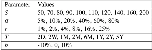
S 50, 70, 80, 90, 100, 110, 120, 140, 160, 200 σ 5%, 10%, 20%, 40%, 60%, 80%

r 1%, 2%, 4%, 8%, 16%, 25%

[image:28.612.143.409.56.131.2]

T 2D, 2W, 1M, 2M, 6M, 1Y, 2Y, 5Y

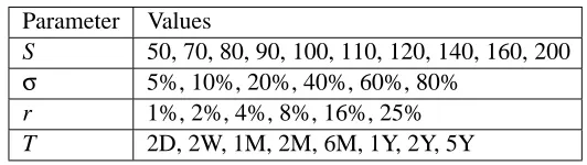
Table 3.2: Parameters for validation scan. The total number of combinations is 2880.

the last two columns show how Q changes for the American call if the optimal nt of the European

case is used. The deterioration is acceptable for the gain in simplicity to use only one relation

noptt =max(100;(ns˜ 100)=2) (3.21)

with an appropriate scaling for the time to maturity of the option. There isn’t much to gain beyond

500 steps in ˜s because the accuracy of the solution of the linear equation system 3.14 is the limiting

factor. Therefore ns˜=500 is chosen for all further studies.

3.3 Validation of the Numerical Solution

A large scale validation of the scheme has been done for equity options. There, analytical solutions

exist for European calls and puts and for American calls with a single discrete dividend. The

pa-rameters shown in table 3.2 were scanned for the validation. Like in the definition of the quality

Q in equation 3.20, only parameter combinations at which the analytical price is above 102 are considered to be not too sensitive to numerical artefacts. The following sections give a summary of

the results. The numbers are summarised in table 3.3. The average deviation is the average of the

relative deviations defined as

V_inum V_iana V_iana

for all parameter combinations i with V_iana>0:01.

For other option underlyings (FX rates, futures), several parameter combinations have been

probed without performing such an extensive study. The tests showed for European options good

agreement so that we can assume that the method is correctly implemented also including

continu-ous dividend yields.

3.3.1 European Calls

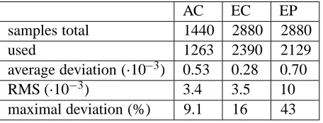
For the European calls, 2390 of the 2880 parameter combinations were accepted with option values

above 10 2. The average relative deviation from the analytical solution was 0:2810

3_{, the largest}

deviation 16% at an option value of 0.025. Deviations larger than 1% occur only at σ=5% and

(29)

3.3. VALIDATION OF THE NUMERICAL SOLUTION 23

AC EC EP

samples total 1440 2880 2880

used 1263 2390 2129

average deviation (10

3₎ _0.53 _0.28 _0.70

RMS (10

3₎ _3.4 _3.5 ₁₀

[image:29.612.194.422.58.145.2]

maximal deviation (%) 9.1 16 43

Table 3.3: Deviation of the finite difference solution from the analytical solution.

3.3.2 European Puts

For European puts, 2129 parameter combinations were accepted. The statistical quantities (espe-cially RMS and maximal deviation) in table 3.3 are dominated by a single large deviation of 43% at an option value of 0.40 with the parametersσ=5%, r=16%, T =5Y and S=50:5. The average

deviation with 0:710

3_{is still well below the goal of 10} 3_{. Deviations above 1% occur only at the}

money forward atσ=5% with high interest rates r16% and at r=8% with T 2Y .

3.3.3 American Calls on Equity with one Discrete Dividend

A dividend of 4 is payed 6 weeks after the valuation date for the American case. (For European options, the dividend makes conceptually no difference.) The last and the first three maturities were skipped for the American call because for the short maturities the dividend wouldn’t fall in the

option lifetime, and for the long maturity the early dividend is of little interest. Therefore only 1440 parameter combinations remain of which 1263 were accepted with option values above 102.

The average deviation is with 0:5310

3 _{slightly higher than for the European calls, but the}

RMS and the maximal deviation are comparable. From the total parameter set probed only 7 lead to deviations>1%, all at the money forward withσ=5% orσ=10% and r8%.

3.3.4 Conclusion

The numerical scheme for the valuation of options has been validated by comparing the results with the analytical solutions for European puts and calls and American calls on equity. An overall (aver-age) accuracy better than 10 3has been achieved over a wide variety of parameter combinations.

Most of the numerical scheme is independent of the presence of continuous dividend yields. There for it is sufficient to check that the yields are correctly implemented with some isolated

parameter combinations. This test has been performed successfully.

(30)

Application of the Methods

Several methods outlined in chapter 2 and defined in the following paragraphs separately for equity

and FX options have been compared to the finite difference scheme described in chapter 3 and selected as a benchmark pricing tool. In the first step the overall performance of the methods was

compared for all parameters and in domains of parameter space (section 4.1). As a second step

those domains were identified in which the methods yield the largest error and where they should not be applied (section 4.2).

The parameters have been set to all combinations of the values shown in table 4.1. The results

of all models viable for the option/underlying combinations were compared to the option value

calculated with the finite differences.

The particular role of equity options in this study is that they can have discrete dividends. The

following methods for pricing American equity options have been compared to the benchmark:

Binomial models with a moderate (200) and a very high (1000) number of time steps in the

binomial tree. They will be called BIN200 and BIN1000, respectively.

The average of binomial trees with 200 and 201 steps as described in section 2.3.3. This

method will be called AVERAGE.

The control variate technique described in section 2.3.4 with a binomial tree with 200 time

steps. The symbol for this method will be CONVAR.

Parameter Values

S 50, 70, 80, 90, 100, 110, 120, 140, 160, 200 σ 5%, 10%, 20%, 40%, 60%, 80%

r 1%, 2%, 4%, 8%, 16%, 25%

T 2D, 2W, 1M, 2M, 6M, 1Y, 2Y, 5Y

[image:30.612.145.407.575.661.2]

b -10%, 0, 10%

Table 4.1: Parameters for the comparison of the methods. The parameter b is varied only for FX

options, and the foreign interest rate is set to q=max(r b;0).

(31)

4.1. COMPARISON OF THE METHODS 25

low domain medium domain high domain

T <0:5y 0:5yT <2y T2y S<90 90S110 S>110

r<4% 4%r8% r>8%

σ<20% 20%σ40% σ>40%

[image:31.612.195.418.56.144.2]

b<0 b=0 b>0

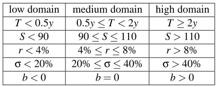
Table 4.2: Parameter domains

The number of time steps of the binomial tree was chosen such that the binomial tree was stable for all studied parameter combinations (i.e. the up–probability p was in the range 0p1).

The models considered for FX options are:

Binomial models BIN200 and BIN1000.

The average of binomial trees with 200 and 201 steps AVERAGE

The control variate technique CONVAR.

The analytic approximation of Barone–Adesi and Whaley (BAW)

The analytic approximation of Bjerksund and Stensland (BJST)

4.1 Comparison of the Methods

The performance of the methods in terms of accuracy and computational efficiency is compared over a broad range of parameters. Also the edges of the realistic parameter space are explored in

order to find the limitations of the different methods. The “true” option value is determined with the finite difference scheme described in chapter 3.

A first comparison of the methods is done on global quantities: The mean of the relative de-viation from the benchmark over all parameter sets, the RMS of the relative dede-viation, and the

maximal relative deviation. In order to study the dependence of the accuracy of the methods on the parameters, each parameter set is divided in three domains. These domains are shown in table 4.2.

4.1.1 Equity Options

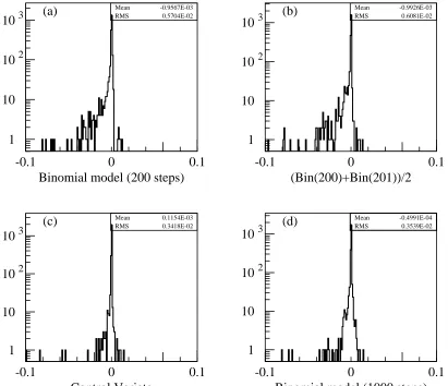
In figure 4.1 the result for American calls is shown as a histogram. The abscissa shows the relative deviation

vmodel vFD

vFD

(4.1)

where vFDdenotes the value of the option calculated with the finite difference scheme and vmodelthe

value calculated with the model indicated in the histogram titles. Each histogram has 2366 entries, and a range of deviations of10% is shown. The statistical quantities can be found in the right

(32)

1

10

2

10

3

-0.1

0

0.1

1

10

2

10

3

-0.1

0

0.1

1

10

2

10

3

-0.1

0

0.1

1

10

2

10

3

-0.1

0

0.1 Binomial model (200 steps)

Mean RMS

-0.9567E-03 0.5704E-02

(a)

(Bin(200)+Bin(201))/2

Mean RMS

-0.9926E-03 0.6081E-02

(b)

Control Variate

Mean RMS

0.1154E-03 0.3418E-02

(c)

Binomial model (1000 steps)

Mean RMS

-0.4991E-04 0.3539E-02

[image:32.612.76.487.62.416.2]

(d)

Figure 4.1: Comparison of the call prices calculated with the method indicated in the histogram

titles with the finite difference solution with a logarithmic scale for the ordinate. Each histogram has 2366 entries.

Some more statistical data can be found in table 4.3. The average deviation is the average of

quantity defined in equation 4.1 over all parameter combinations i with V_iFD>0:01. Obviously, the

binomial models BIN200 and AVERAGE tend to yield too low values. The methods CONVAR and BIN1000 are on average very close to the finite difference solution. The RMS shows that these two

have about the same accuracy globally. The means don’t differ significantly. However, in terms of computation time1, the method CONVAR is about 28 times more efficient.

The analysis of the parameter domain shows that BIN1000 is superior to CONVAR only for

short–term at–the–money calls at high rates and low volatility, for medium term at–the–money and in–the–money calls at low rates and medium volatility, and for long–term in-the-money calls at low rates and low volatility.

1_{All computation times are measured on a K6-III/400 system running Linux kernel 2.2.5 and the GNU compiler suite}

(33)

Method BIN200 AVERAGE CONVAR BIN1000

average deviation(10

3

) -0.96 -0.99 0.11 -0.05

RMS of deviations(10

2

) 0.57 0.61 0.34 0.35

number of deviations>1% 108 96 15 23

largest deviation 33% 33% 10% 14%

[image:33.612.129.483.57.146.2]

computation time (s) 29 60 28 777

Table 4.3: Statistical data for calls on equity

Method BIN200 AVERAGE CONVAR BIN1000

average deviation(10

3

) -1.27 -1.28 -0.49 0.28

RMS of deviations(10

2

) 0.68 0.67 0.58 0.27

number of deviations>1% 130 126 68 18

largest deviation 47% 47% 47% 7%

[image:33.612.127.483.188.279.2]

computation time (s) 29 61 29 795

Table 4.4: Statistical data for puts on equity

The methods BIN200 and AVERAGE deviate at 108 and 96 parameter combinations,

respec-tively, from the benchmark by more than 1%. These parameter combinations are scattered over a

wide domain of parameter space; therefore their distribution hasn’t been studied further.

The 15 parameter combinations for CONVAR with deviations above 1% are shown in appendix

C.1.1. Almost all these combinations have a low volatility10% and a high interest rate r16%.

These combinations are unrealistic for most practical purposes. Only three combinations occur at

lower rates, but also at the low volatilityσ=5% out of the money.

In Appendix C.1.2 the parameter combinations are summarised for which method BIN1000

yields a deviation greater than 1%. The overall distribution of these parameter combinations is

similar to that of CONVAR. All the additional critical parameter combinations occur far out of the

money at low volatility and high rate or long time to maturity.

Figure 4.2 shows the equivalent results for puts on equity. The summarising statistical data are

displayed in table 4.4. All methods are significantly less accurate than for calls. Especially method

CONVAR has a maximal deviation of the same size as BIN200 and AVERAGE. As can be seen in

the table of appendix C.2.1, the prices of in-the-money options with long times to maturity are not

very good, in addition to the critical regions of the calls. The reason is that for equity puts, early exercise of the American option is much more important than for calls. Therefore, the difference

between the price of an American put and a European put is larger than between the price of an

American call and a European call. As this difference gets large, the correction introduced by the

binomial tree calculation of American and European put gets larger, and the numerical error (of the

same magnitude as in BIN200 and AVERAGE) becomes more important. However, the average deviation and the RMS are still significantly better than for those two methods, and the number of

(34)

1

10

2

10

3

-0.1

0

0.1

1

10

2

10

3

-0.1

0

0.1

1

10

2

10

3

-0.1

0

0.1

1

10

2

10

3

-0.1

0

0.1 Binomial model (200 steps)

Mean RMS

-0.1267E-02 0.6781E-02

(a)

(Bin(200)+Bin(201))/2

Mean RMS

-0.1281E-02 0.6732E-02

(b)

Control Variate

Mean RMS

-0.4936E-03 0.5757E-02

(c)

Binomial model (1000 steps)

Mean RMS

0.2835E-03 0.2748E-02

[image:34.612.76.488.62.419.2]

(d)

Figure 4.2: Comparison of the put prices with the finite difference solution with a logarithmic scale

for the ordinate. Each histogram has 2189 entries.

Compared with BIN1000, CONVAR performs much worse in many parameter domains. These

domains are scattered all over the parameter space. Clearly the best method for puts on equity is BIN1000 that yields even less deviations than for calls, at the cost of a high computational effort.

4.1.2 FX Options

The methods considered here have already been summarised in the beginning of this chapter. There is yet another parameter to be varied, the foreign interest rate (or dividend yield for index options)

q. This parameter has been chosen to be q=max(r b;0)where the cost of carry b was chosen as

-10%, 0 (corresponding to futures options) and +10%. Therefore there are in total 8640 parameter combinations.

For 7022 combinations the call price is >0:01. The overall result for calls is shown in table

(35)

1

10

2

10

3

-0.1

0

0.1

1

10

2

10

3

-0.1

0

0.1

1

10

2

10

3

10

4

-0.1

0

0.1

1

10

2

10

3

10

4

-0.1

0

0.1

1

10

2

10

3

-0.1

0

0.1

1

10

2

10

3

-0.1

0

0.1 Binomial model (200 steps)

Mean RMS

-0.6229E-03 0.5140E-02

(a)

(Bin(200)+Bin(201))/2

Mean RMS

-0.5349E-03 0.4849E-02

(b)

Control Variate

Mean RMS

0.1844E-03 0.2818E-02

(c)

Binomial model (1000 steps)

Mean RMS

0.1947E-03 0.2598E-02

(d)

Barone-Adesi-Whaley

Mean RMS

0.5849E-02 0.1595E-01

(e)

Bjerksund-Stensland

Mean RMS

-0.2289E-02 0.5337E-02

[image:35.612.105.516.63.633.2]

(f)

Figure 4.3: Distribution of deviations for American calls on FX rates rates with a logarithmic scale

Valuation of American Options