H. Lundstedt1, T. Persson2, and V. Andersson1 1Swedish Institute of Space Physics (IRF), Lund, Sweden
2Centre for Mathematical Sciences, Lund University, Lund, Sweden Correspondence to: H. Lundstedt ([email protected])
Received: 4 June 2014 – Revised: 19 November 2014 – Accepted: 29 December 2014 – Published: 27 January 2015
Abstract. A complex solid torus model was developed in or-der to be able to study an extreme solar storm, the so-called “Great Storm” or “New York Railroad Storm” of May 1921, when neither high spatial and time resolution magnetic field measurements, solar flare nor coronal mass ejection obser-vations were available. We suggest that a topological change happened in connection with the occurrence of the extreme solar storm. The solar storm caused one of the most severe space weather effects ever.
Keywords. Solar physics astrophysics and astronomy (mag-netic fields)
1 Introduction
Today’s high-tech society has become very vulnerable to strong solar storms, such as coronal mass ejections (CMEs) and solar flares. Fast Earth-directed CMEs may cause se-vere geomagnetic storms with large dB/dt variations and accompanied problems for the power industry (Lundstedt, 2006). Intense solar flares may cause problems for HF com-munications and aviation. Sixteen regional warning centres (RWCs) within the International Space Environment Ser-vice (ISES) provide world-wide forecast serSer-vices of solar storms and space weather effects. RWC-Sweden (Swedish Space Weather Center) is operated by the Swedish Institute of Space Physics (IRF), in Lund. We offer warnings and fore-casts based on space- and ground-based observations. Agen-cies around the world, among them the Swedish Civil Con-tingencies Agency (MSB), now work together in order to prepare for severe space weather effects. However, the latest research and observations show that we lack the necessary knowledge to understand and warn for extreme solar storms
and possible severe geoeffects. Historical records and astro-nomical observations of solar-type stars also tell us that we may be exposed to much stronger solar storms in the future. Flares up to a thousand times stronger have been observed on a solar-like star (Maehara et al., 2012). It is important to have warning of severe/extreme solar storms several days ahead, far enough in advance to be able to take action. Recent studies of extreme solar storms (Cannon, 2013) suggest that they occur much more often than just every 150 years and also that they can occur at any time during the sunspot cycle, i.e. not just close to solar maximum; they can occur even dur-ing weak sunspot cycles such as the present solar cycle 24. The most famous extreme solar storm, in September 1859, occurred during a weak cycle. This event, the so-called Car-rington event, is often used as a measure of the most extreme solar storm and has been called a super solar storm. However, at that time solar magnetic fields were not measured, making it difficult to classify as an extreme solar storm (Lundstedt, 2010, 2012). In 1908 George Hale at Mount Wilson (MW) Observatory was able to measure the solar magnetic field us-ing the Zeeman effect, a breakthrough in the search for a pat-tern behind solar activity and solar storms. In this paper we describe an attempt to use changes of the magnetic complex-ity to understand the extreme solar storm of May 1921, the first extreme event for which solar magnetic field measure-ments are available.
2 Solar observations
110 H. Lundstedt et al.: The extreme solar storm of May 1921
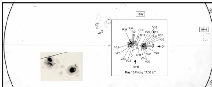
Figure 1. Mount Wilson drawing of active regions occurring on 13 May 1921 at 17:30 UT and to the left, a white-light observation by Royal Greenwich Observatory (RGO) at 09:55 UT.
up until 19 May at 61◦ on the west limb. Only the group following the Hale polarity law survived to the next rotation and appeared at the centre of the Sun on 10 June (Tamm, 1922). As can be seen in Fig. 1, only one small active region (AR 1844) appeared at the same time. Whether connected activity took place on the Earth-facing side of the Sun or not is hard to tell since the observer focused on AR 1842 (Title, 2012).
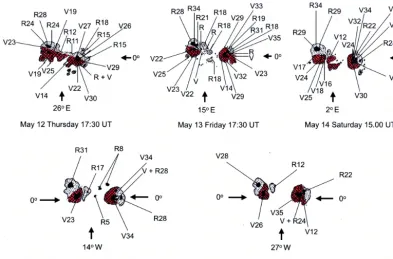
The active region 1842 in 12–16 May 1921 (RGO, 1955; Silverman and Cliver, 2001; Tamm, 1922) showed magnetic complexity(β–γ )and was located between 26◦E and 27◦W longitude at low latitude (Fig. 2). The spot group, Greenwich number 9334, had a large mean area of 1324 millionths of the Sun’s visible hemisphere. The region 9334 with three large sunspots showed large flux changes especially on 12 May, but fluxes also disappeared and new fluxes emerged on 13 and 14 May 1921. The observer Eddison Petit at Mount Wil-son made a note on the drawing that both H-alpha and K lines were bright, i.e. we also had strong solar flares on 12 May. We also notice a rotation of both sunspot groups, from hav-ing a line of polarity separation parallel to the equator to one perpendicular to it. When the large region after 12 May was broken up into two regions, the left started to rotate counter clockwise and the right clockwise. New negative flux was also seen to emerge on 14 May. Mount Wilson measured very strong magnetic flux densities of between +0.34 and
−0.35 T (Fig. 2). These values have been corrected (Liv-ingston et al., 2006) to +0.35 and−0.36 T. We notice that reduction of magnetic complexity took place at the times of the solar storms. Interestingly, Schrijver (2009) suggests in his review that the emergence of twisted flux ropes into pre-existing strong field plays a critical role for many, if not all, of the active regions that produce M- or X-class flares. As for the Carrington event, the solar storms 9334 in 1921 oc-curred during a moderate sunspot cycle and during the de-clining phase of cycle 15.
3 Terrestrial effects
Geomagnetic storm activity occurred mainly at about 20:00 UT on 13 May (Royal Greenwich Observatory, 1955), at 21:00–24:00 UT on 14 May and at 04:00–06:00 UT on 15 May (Silverman and Cliver, 2001). A sudden commence-ment (S.C.) and arrival of the first CME occurred at 13:10 UT on 13 May (Royal Greenwich Observatory, 1955). The next S.C. occurred at 22:20 UT on 14 Ma (Silverman and Cliver, 2001) and signalled the arrival of a new CME. The first CME may have cleared the way for the second one in the same way as occurred in an extreme solar storm on 23 July 2012 (Baker et al., 2013). Interestingly, a value for the rate of change of the horizontal component of the geomagnetic field dBh/dt as high as about 5000 nT min−1has been estimated for 14–15 May in Sweden (Kappenman, 2006). At 00:00 UT (02:00 local time) in the morning of 15 May a fire occurred in a telegraph station in Karlstad, Sweden (Em, 1921). Au-rora was observed as close to the magnetic equator as Samoa (Silverman and Cliver, 2001), making the 1921 event one of the strongest space weather events ever reported.
4 Complex topological models
In order to be able to study an extreme solar storm, such as the one in May 1921, i.e. before high spatial and time-resolved vector magnetic field measurements and velocity measurements existed, we developed a complex torus model. The complexity is mathematically produced by an iterative mapping of a torus of magnetic flux tubes (Fig. 3).
A complex solid torus (Devaney, 2003) model was devel-oped in order to address three questions:
Figure 2. Active region 1842 observed at the Mount Wilson Observatory between 12 and 16 May 1921. V stands for negative magnetic field and R for positive. V25 e.g. corresponds to−0.25 T or corrected−0.24 T (Livingston et al., 2006). Large hatched areas of negative polarity are coloured red. When the large region after 12 May is broken up into two regions, the left starts to rotate counter-clockwise and the right clockwise. New negative flux is also seen to emerge on 14 May.
2. Can the solid torus model be used to reconstruct mag-netograms and also make a study of the evolution of the active regions?
3. Can a probable explanation be found of the extreme so-lar storm of May 1921?
Let us start with the first question.
4.1 A complex solid torus model of magnetograms and information extraction
We can parameterize the torusTwith the coordinates(θ, z)
where 0≤θ <2π andz∈C,|z| ≤1. Leta be an integer,
a≥1,b∈C,|b|<1,c∈C, andd an integer,d≥1 (unless
a=1 in which cased≥0) and gcd(a, d)=1 (Fig. 3 to the left).
Consider the map (Katok and Hasselblatt, 2006)
F :(θ, z)7−→(aθ, bz+ceidθ). (1) HenceF maps the torus into a torus that has been “folded”a
times.
We assume that b andcare chosen so that F maps the torus into itself. Consider the setF (T)at the sectionθ=θ0. The parametera is the number of connected components of
F (T).
Figure 3. A torusTis parameterized with the coordinates(θ, z)to the left and a mapped cross-section is shown to the right.
The preimages of the points inF (T)at the sectionθ=θ0 are the points with
θ=θ0
a +
2π
a k, k=0,1, . . ., a−1. (2)
Hence, the section ofF (T)atθ=θ0is the set
{bz+ceid(θ0/a+2π k/a): |z|<1, k=0,1, . . ., a−1}. (3) We can therefore get some information about the param-eters according to the picture to the right in Fig. 3. For
k=0,1, . . ., a−1 we have
φk=γ+d
θ0
a +
2π a k
, (4)
[image:3.612.309.545.404.488.2]112 H. Lundstedt et al.: The extreme solar storm of May 1921
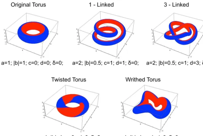
Figure 4. The first solid torus to the left shows the original torus. By changing the parameterdto 1 or 3 we obtain a one- or a three-linked torus. By changingδfrom 0 to 2 for the original torus we obtain a twisted torus. Finally by changing thecto 1 anddto 3 for the original torus we obtain a writhed torus.
We have now seen that we can extract complexity param-eters from a picture.
Let us now address the second question and try to repro-duce magnetograms from different values of these complex-ity values for the torus.
4.2 Reconstruction of magnetograms using the torus model
Withb= |b|eiδwe can write the mapF as
F (θ, z)=(aθ,|b|eiδz+ |c|eiγ+idθ). (5) By changing the values ofa,b,c,dand the angleθwe can describe byFn(T), where the number of iterationsnis a
pos-itive integer, a linked, a twisted and writhed solid torus. The parameteradescribes how many times the curve winds about the centre,|b|changes the thickness of the image of the solid torus,|c|determines the separation of the solid torus parts in the cross-sectional planes,(a−1)dis the linking number of the image of the solid torus and finally the parameterδ deter-mines the twist of the torus. The solid torus is then cut along its circular axis in two parts. These are the blue and red parts shown in Fig. 4. The two parts will be treated as positive and negative poles.
In Fig. 4 we give a couple of examples. The first solid torus to the left shows the original torus. By changing the param-eterd to 1 or 3 we obtain a one- or a three-linked torus. By changing δ from 0 to 2 for the original torus we obtain a twisted torus. Finally by changing thecto 1 andd to 3 for the original torus we obtain a writhed torus.
We cut the torus at an angleθ and then calculate a simu-lated magnetogram from this cut as follows: for each pointy
in the simulated magnetogram, the intensity is given by the integral
Z
ρ(x)|y−x|−2dV (x),
where the integral is over all pointxin the cut, and dV de-notes the area measure. The functionρ(x)is defined to be 0 ifxis outside the torus, andρ(x)= ±1 depending on which part of the torusx is in. In the computer, this integral is ap-proximated by a finite sum.
We can also simulate magnetograms at any time in be-tween. The colour code has been chosen to be the same as for observed HMI, SDO magnetograms. The most simple simu-lated magnetogram is obtained by taking a cut of the orig-inal torus into two adjacent tori with halved cross-sectional area (treated as positive and negative poles) and a grid of values is calculated based on their inverse distance squared. We may then e.g. map the torus once (n=1), and take cuts atθ=120◦orθ=360◦and obtain the other magnetograms (Fig. 5).
The solenoid is an attractor which is contained in a “solid torus” (Devaney, 2003). We would therefore expect iterating
F should produce fractal magnetograms.
The magnetograms in Fig. 6 show exactly that.
Figure 5. The most simple simulated magnetogram is obtained by taking a cut of the original torus into two equal semicircles (treated as positive and negative poles) and a grid of values is calculated based on their inverse distance squared to the semicircles. We may then e.g. map the torus once (n=1), and take cuts atθ=120◦orθ=360◦and obtain the other magnetograms.
Figure 6. By iterations of the torus model we can obtain the fractal structure of magnetograms.
several connected tori. In the next and final example of May 1921 we use four connected tori.
4.3 Reconstruction of the magnetograms describing the extreme solar storm of 1921
Finally, we address the third question. We will reproduce the magnetograms of May 1921 and then try to understand what caused the extreme solar storm and when it occurred.
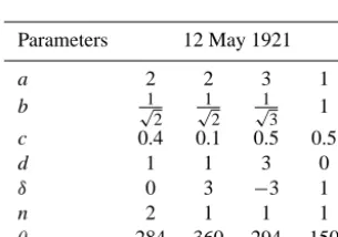
We use four tori to reproduce the magnetograms for 12 to 16 May (Fig. 8). It is assumed that these four tori are con-nected. The parameter sets used are displayed in Table 1.
We start with 12 May at 18:00 UT and after the break-up into two major regions which seems to have taken place on 13 May UT morning. We then try to reproduce the changes in the magnetograms topologically, i.e. by continuous change of
θ andz. On 13 May the left region starts to rotate anticlock-wise to follow the Hale law. The right region starts to rotate clockwise. On late 13 to early 14 May we notice both emerg-ing of flux and large rotations especially for the active
re-Figure 7. Two HMI magnetograms observed by SDO on 13 and 29 March 2013. Below are the parameters to give a solid torus model that can simulate the magnetograms.
[image:5.612.76.259.319.433.2]114 H. Lundstedt et al.: The extreme solar storm of May 1921
Figure 8. Simulated magnetograms from 12–16 May 1921. On 13 May the active regions start to rotate and new flux emerges.
Table 1. The set of parameters of the four tori used to simulate the magnetogram of 12 May 1921.
Parameters 12 May 1921
a 2 2 3 1
b √1
2 1 √ 2
1 √
3 1
c 0.4 0.1 0.5 0.5
d 1 1 3 0
δ 0 3 −3 1
n 2 1 1 1
θ 284 360 294 150
4.4 Further research
There are many possible extensions of the solid torus ap-proach. A natural extension is to start trying to reconstruct magnetograms of higher time and spatial resolution, such as the magnetograms produced by HMI onboard SDO (Hoek-sema et al., 2014), something we have already prepared for. With measurements of vector magnetic fields we will be able to make estimation of the energy release and give a better description of the magnetic complexity.
It would be very interesting to try to estimate the energy released during the extreme solar storm based on the change of the complexity parameters of the torus. Berger (1993) es-timated that the free energyEm, stored in the braided field, is proportional to the square of the crossing numberCmin:
Em≥9.06×10⁻²C2min
82
N2L, (6)
where8is the magnetic flux of the flux tubes,N the number of strands of the braid (=flux tubes) andLthe length. The linking numbers are closely related to the average crossing number, which is an algebraic measure of the link complexity in space (Ricca, 2002). Interestingly it is also found (Berger and Asgari-Targhi, 2009) that the energy released due to
re-connection of the braids in the coronal loops follows a power-law distribution, i.e. is fractal.
We have used several solid tori to describe large complex active regions and the evolution. It would also be interest-ing to study the small–large-scale magnetic field couplinterest-ing as seen at times of solar flares and the Hale Solar Sector Bound-ary (Svalgaard et al., 2011; Lundstedt et al., 1980).
[image:6.612.91.244.298.405.2]5 Summary
Magnetic field measurements carried out at the Mount Wil-son Observatory as long ago as 1908 have made it possible for us to interpret the extreme solar storm in May 1921 based on the change and complexity of the magnetic field. In this paper we describe an attempt based on a complex solid torus model. A topological change is suggested at the time of the extreme solar storm. The model also makes it possible to study the development of an active region. The model will be further developed in order to even make use of today’s magnetic field measurements by HMI onboard SDO (Hoek-sema et al., 2014). The use of the SHARP service (Bobra et al., 2014) would make it operational. Being able to warn when a severe solar storm will develop into an extreme one is of great importance in order to be able to mitigate the effects for society.
Acknowledgements. We thank Todd Hoeksema and the SDO HMI solar team at Stanford, the SDO AIA team at Lockheed, the SOHO team, the Mount Wilson Observatory, Sarah Matthews, Univ. Col-lege London, Dept. of Space & Climate Phys. Solar & Stellar Physics Group, Mullard Space Science Laboratory for RGO 1921 for the data used, and geomagnetic field data for dB/dtestimations from World Data Centre Geomagnetism, British Geological Sur-vey (BGS), Edinburgh, Instituto Nazionale di Astrofisica (INAF), Catania, Italy and NOAA Space Weather Prediction Center, USA. Finally we thank two referees, Mauro Messerotti and one anony-mous, for helping to improve the paper.
Topical Editor M. Temmer thanks M. Messerotti and one anony-mous referee for their help in evaluating this paper.
References
Baker, D. N., Li, X., Pulkkinen, A., Ngwira, C. M., Mays, M. L., Galvin, A. B., and Simunac, K. D. C.: A major solar eruptive event in July 2012: Defining extreme space weather scenarios, Space Weather, 11, 585–591, 2013.
Berger, M.: Energy-Crossing Number Relations for Braided Mag-netic Fields, Phys. Rev. Lett., 70, 705–708, 1993.
Berger, M. A. and Asgari-Targhi, M.: Self-organized braiding and the structure of coronal loops, Astrophys. J., 705, 347–355, 2009.
S., Norton, A., Bobra, M., Centano, R., Leka, K. D. Barnes, G., and Turmon, M.: The Helioseismic and Magnetic Imager (HMI) Vector Magnetic Field Pipeline: Overview and Performance, Sol. Phys., 289, 3483–3530, doi:10.1007/s11207-014-0516-8, 2014. Kappenman, J. G.: Great geomagnetic storms and extreme
impul-sive geomagnetic disturbance events – An analysis of observa-tional evidence including the great storms of May 1921, Adv. Space Res., 38, 188–199, 2006.
Katok, A. and Hasselblatt, B.: Introduction to the modern theory of dynamical systems, Encyclopedia of Mathematics and its Appli-cations, edited by: Rota, G.-C., Vol. 54, Cambridge, 2006. Livingston, W., Harvey, J. W., and Malanushenko, O. V.: Sunspots
with the strongest magnetic fields, Sol. Phys., 239, 41–68, 2006. Lui, Y. D., Luhmann, J. G., Kajdic, P., Kilpua, E., Lugaz, N., Nitta, N. V., Möstl, C., Lavraud, B., Bale, S. D., Farrugia, C. J., and Galvin, A. B.: Observations of an Extreme Storm in Interplan-etary Space Caused by Successive Coronal Mass Ejections, Na-ture Communications, 5, 3481, 2014.
Lundstedt, H.: The Sun, space weather and GIC effects in Sweden, Adv. Space Res., 37, 1182–1191, 2006.
Lundstedt, H.: Solar storms, cycles and topology, Eur. Phys. J., 9, 95–103, 2010.
Lundstedt, H.: Solar storms and topology: Observed with SDO, in: Proceedings of TIEMS conference “Space Weather and Chal-lenges for Modern Society”, 22–24 October 2012.
Lundstedt, H. and Persson, T.: Modelling solar cycle length based on Poincaré maps for Lorenz-type equations, Ann. Geophys., 28, 993–1002, doi:10.5194/angeo-28-993-2010, 2010.
Lundstedt, H., Wilcox, J. M., and Scherrer, P. H.: Geomagnetic Ac-tivity and Hale Sector Boundaries, Planet Space Sci., 29, 167– 170, 1980.
Maehara, H., Shibayama, T., Notsu, S., Notsu, Y., Nagao, T., Kus-aba, S., Honda, S., Nogami, D., and Shibata, K.: Superflares on solar-type stars, Nature. Letter, 485, 478–481, 2012.
Ricca, R. L.: Energy, helicity and crossing number relations for complex flows, in: Tubes, Sheets and Singularities in Fluid Dy-namics, edited by: Bajer, K. and Moffatt, H. K., 139–144, Kluwer Academic Publishers, the Netherlands, 2002.
Royal Greenwich Observatory: Sunspot and Geomagnetic-Storm Data, derived from Greenwich observations, 1874–1954, Lon-don: Her Majesty’s Stationary Office, 1955.
Schrijver, C. J.: Driving major solar flares and eruptions: A review, Adv. Space Res., 43, 739–755, 2009.
116 H. Lundstedt et al.: The extreme solar storm of May 1921
Svalgaard, L., Hannah, I. G., and Hudson, H.: Flaring solar Hale Sector Boundaries, Astrophys. J., 733, 49, doi:10.1088/0004-637X/733/1/49, 2011.
Tamm, N.: Die grossen Sonneflecken Mitte Mai und Anfang Juni 1921, Astron. Nachr., 215, 209–212, 1922.
Title, A.: Remote Triggering of Energetic Events, in: Proceedings of TIEMS conference “Space Weather and Challenges for Modern Society”, 22–24 October 2012.
Török, T., Berger, M. A., and Kliem, B.: The writhe of helical structures in the solar corona, Astron. Astrophys., 516, 11 pp., doi:10.1051/0004-6361/200913578, 2010.