SRef-ID: 1432-0576/ag/2005-23-2249 © European Geosciences Union 2005
Annales
Geophysicae
On the development and evolution of nonlinear ion acoustic wave
packets
A. M. Hamza
Physics Dept., University of New Brunswick, POB 4400, Fredericton, E3B 5B-5A3, Canada
Received: 29 March 2005 – Revised: 6 June 2005 – Accepted: 8 June 2005 – Published: 15 September 2005
Abstract. A simple model of ion fluctuations (ion acoustic
and ion cyclotron fluctuations for example) driven by an elec-tron current which leads to intermittent fluctuations when the linear growth rate exceeds the wave packet dispersion rate is analized. The normalized fluctuation amplitudeeφ0/T can
be much larger than the mass ratio(me/mi)level predicted by the conventional quasilinear theory or Manheimer’s the-ory (see references in this document), and whereφ0
repre-sents the amplitude of the main peak of the ion fluctuations. Although the ion motion is linear, intermittency is produced by the strong nonlinear electron response, which causes the electron momentum input to the ion fluctuations to be spa-tially localized. We treat the 1-D case because it is espe-cially simple from an intuitive and analytical point of view, but it is readily apparent and one can put forward the conjec-ture that the effect occurs in a three dimensional magnetized plasma. The 1-D analysis, as shown in this manuscript will clearly help identify the subtle difference between turbulence as conventionally understood and intermittency as it occurs in space and laboratory plasmas.
Keywords. Meteorology and atmospheric dynamics
(Tur-bulence) – Ionosphere (Wave-particles interactions) – Space plasma physics (Waves and instabilities)
1 Introduction
1.1 Historical background
Isolated coherent fluctuations have been observed in both physical and simulation plasma. When such fluctuations are formed randomly in the presence of lower level background turbulence, the turbulence is called intermittent. A quantita-tive measure of intermittency is the Kurtosis, which is a mea-sure of the flatness of the probability distribution function (see for example Frisch, 1995). There are many examples of such intermittent fluctuations, but here we shall be mainly
Correspondence to: A. M. Hamza
interested in a very simple example, namely 1-D ion fluctu-ations driven by an electron current (in the ion acoustic and ion cyclotron regimes), illustrating the development of large and coherent ion fluctuations in a current driven plasma. Our preliminary studies indicate that the 1-D effects dealt with here persist when extended to the case of a 3-D plasma in a magnetic field (see for example Hamza, 1988, 1993). Al-though the 1-D model is limited in direct application to phys-ical problems, this deficiency is more than compensated for by the relative simplicity of the analytic treatment and the more definitive and unambiguous nature of the relevant com-puter simulations. It is also illuminating that even in this simplest of cases, the conventional theoretical understanding is wrong.
Sato and Okuda (1979,1981) were apparently the first to observe such fluctuations in numerical simulations. Barnes et al. (1985) obtained similar results but provide much more detailed phase space information. Berman et al. (1986) ex-tended the work to include additional diagnostics and to show that such fluctuations could occur in linearly stable plasma. These simulations were motivated, in part, by satellite obser-vations (see for example Koeskinen et al. (1988) and Mozer et al. (1982)) of isolated large amplitude fluctuations in au-roral plasma thought to be driven by an electron current (see for example Mozer et al. (1982)). More recently a number of satellite observations from Freja and FAST have clearly iden-tified intermittent, spatially localized ion fluctuations (see for example Potelette et al. (2004) and references therein).
Figure 1: A symmetric wave Packet illustration with maxima and minima. φ0
φ1
φ2
φ3
x0
x1
x2
x3
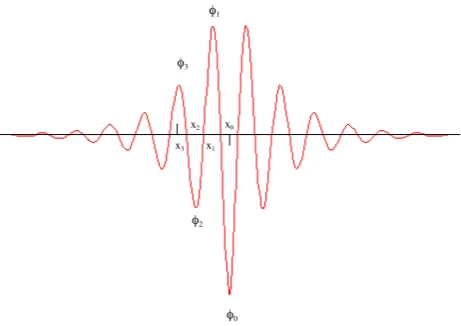
Fig. 1. A symmetric wave Packet illustration with maxima and min-ima.
There are essentially two questions to be addressed. First, how can the fluctuations grow to the large amplitudes, of order e|φ0|/T≈1 (noting that large amplitudes can
exceed the value of one), observed in the simulations when the conventional analysis predicts amplitudes of order e|φ0|/T≈me/mi or less? (φ0, which is negative in the case
of interest, is the value of the potentialφ (x)at its maximum amplitude (see Fig. 1), T is the electron temperature, and the other symbols have their usual meaning.) And secondly, what is the physical nature of the localized ion fluctuation? 1.1.1 Conventional answers
The first question involves electron free energy (or momen-tum) and the relaxation of the electron distribution func-tion by the potential fluctuafunc-tions (see for example reference Dupree, 1986). Historically there have been two treatments of this question depending on the ratio of the fluctuation au-tocorrelation rateγcto the electron reflection or trapping rate γe. When γcγe, quasi linear theory applies and predicts that the ultimate fluctuation level (in a closed system) is very small, of ordere|φ0|/T≈me/mi or less. Manheimer (1971)
has analyzed the other limit,γcγe. His analysis predicts that the ultimate value of the potential is of the same order as the previous case.
That these two seemingly disparate approaches should both predict very small final fluctuation amplitude is not sur-prising. In both cases, the growth of the ion fluctuation is de-termined by the momentum lost by the relaxation (“plateau-ing”) of the electron distribution function over a small frac-tion of its width in velocity space, i.e. of order(me/mi)1/2 or less. Quasilinear theory and the Manheimer theory treat a problem in which ion fluctuations are closely packed and fill the physical space. When the momentum lost by the elec-trons is uniformly allocated to the closely packet ion fluctu-ations to determine the amount absorbed by each fluctuation and therefore the amplitude of each fluctuation, one obtains the amplitude estimates given above.
1.1.2 The intermittency argument
Consider, however, the case in which the ion fluctuations are not closely packed. It is obvious that if the same amount of lost electron momentum is allocated to a smaller num-ber of isolated ion fluctuations, the amplitude of each fluc-tuation must necessarily be larger. Furthermore there is an additional effect that leads to an even greater enhancement of fluctuation level. The momentum imparted to the ions comes from the relaxation of the electron distribution func-tion over a velocity interval,1ve, equal to the trapping width (e|φ0|/me)1/2. In the isolated fluctuation case the potential is no longer limited to a small value and as it increases so does the electron trapping width and therefore the electron free momentum available to drive the ion fluctuations. The amplitude pulls itself up by its bootstraps.
Following the conventional approach (see for example Drummond, 1965; Kadomtsev, 1965), one can make an ap-proximate estimate of the final amplitude for isolated fluctua-tions by generalizing Manheimer’s argument. We consider a plasma which initially contains an electron current and an ar-ray of negative potential pulses a distancedapart (see Fig. 1). In the rest frame of the potential pulses, an electron whose speed is less than the trapping width 1ve≈(e|φ0|/me)1/2 will be reflected by the potential pulses. Electrons moving in both directions will be reflected, but because there is a current, there will be a net momentum loss by the electrons and therefore a net momentum gain by the ion pulses and consequently the ion fluctuations will grow. As the pulse po-tential grows so does the maximum electron speed,1ve, that can be reflected. If the potential is growing exponentially at the rateγ, then during each successive time interval of lengthγ−1the potential increases by a factor ofetimes its previous value and a whole new additional group of electrons can be reflected. This process will continue until the bulk of the electrons being reflected by a pulse have been previously reflected by another pulse. This would require that in one time interval,γ−1, a reflected electron traveled a distanced. Thus the fluctuations will cease growing whenγ−11ve≈d. If the fluctuations are not isolated, but consist of an infinite wave train, thendis set equal to the reciprocal wavenumber kand one obtains Manheimer’s criterion. On the other hand sinceφ0∝1ve2, makingd>k−1enhances the potential fluc-tuation over the Manheimer value by the factor(kd)2. By makingdsufficiently large one may obtain fluctuations with e|φ0|/T≈1, or larger, as convincingly demonstrated by the
simulations.
and are therefore driven by, electrons whose speeds are too great for them to have been reflected by smaller fluctuations, so the growth of the big fluctuations is not inhibited by the smaller ones. On the other hand, the converse is not true, the larger fluctuation do shadow the smaller ones and de-prive them of momentum. Therefore as time evolves, only progressively larger fluctuations survive, and these, of neces-sity, must be progressively further apart since otherwise they would have shadowed each other at an earlier epoch in their growth and could not have grown to large amplitude. It is a case of “survival of the fittest”.
1.1.3 The ion acoustic wave packet case
The point of the preceding discussion is that if isolated fluc-tuations exist, one can explain their apparent anomalously large amplitude. The open issue, to be addressed here, is to explain the nature of the observed ion fluctuations when they still have small amplitude, are localized, and have a nega-tive potential peak. Not only is the neganega-tive potential peak observed in the auroral and simulation plasma, but it is the-oretically necessary in order to reflect electrons and thereby obtain a momentum input to the fluctuations to make them grow. There are several obvious candidates for the observed fluctuations. As mentioned earlier, BGK holes qualify, but we are interested in amplitudes which are too small to trap ions. Another candidate, frequently proposed in the litera-ture, are Kd.V solitons. However these fail on several counts. First the compressive Kd.V soliton has a positive potential peak, not the required negative peak. Also the Kd.V soliton propagates with a speed that is amplitude dependent contrary to the results of the simulations. Finally the localization of the compressive Kd.V soliton is achieved by balancing the dispersion against ion nonlinearities. However, the simula-tions show localized fluctuasimula-tions at small amplitudes where the ions are linear.
Another possibility is a linear wave packet. This candidate would also appear to fail since dispersion will cause such a packet to decay in amplitude and spread out in space at a rateγdwhich is rapid compared to the observed lifetimes in the simulations. Nevertheless it is possible to make the lin-ear wave packet work. The principal result of this paper is that when the linear growth rate exceeds the dispersion rate, an electron nonlinearity (as contrasted to an ion nonlinearity) will counteract the effects of dispersion and keep the fluctu-ation localized.
The physical basis of this effect is quite simple, although unexpected. In Sect. 2 we consider electron reflection and trapping in a growing wave packet consisting of a central peak with progressively smaller ”foothills” (lower amplitude wave packet peaks, see Fig. 1) on either side of the main peak. We show that, although electron reflection occurs at all peaks including the main peak, the net momentum in-put to the ions occurs only around the main peak. Since, for linear ions, fluctuation amplitude is proportional to mo-mentum content, this means that the electrons drive only the main peak of the wave packet. There is no momentum
input by the electrons to the “foothills” since the input by re-flected electrons is canceled by electrons trapped between the “foothills”. As the electrons feed momentum into the main peak, dispersion will feed momentum into the foothills caus-ing their amplitude to grow. However, if electron momentum is fed into the main peak faster than it is lost by dispersion, the main peak will grow.
1.1.4 Linear theory of ion acoustic instability
The linear theory of ion acoustic waves is elementary and well known so we shall only quote the results here. For a wave of frequencyωand wavenumberk, the real part of the appropriate dielectric function forviω/ kveis
R(k, ω)=1+(k2λ2D)
−1−ω2
pi/ω
2 (1)
whereR,λD, andωpiare the real part of the dielectric func-tion, the electron Debye length and the ion plasma frequency respectively. SettingR=0 produces the dispersion relation ω2k =k2c2s(1+k2λ2D)−1 (2) wherecs=ωpiλD=(T /mi)1/2is the sound speed. When the imaginary part of is small, the linear growth rate of ion acoustic wavesγ`is given by
γ` =(π/2)kcsve2f
0
0e(u) (3)
where ve=λDωpe is the electron thermal speed, f00e(u)=(∂/∂u)f0e(u), and f0e(u) is the unperturbed electron distribution function evaluated at the phase speed of the wave packetu=ω/ k.
The broadening of a linear wave packet due to dispersion is treated in reference (Jackson, 2000), but the essential re-sults are easy to derive by approximate arguments. We de-fine the dispersion rate γd as one-half the rate of increase of the logarithm of the width of the wave packet. For a wave packet containing a wave number spread of 1k, the spread in group velocity is 1k(∂2ωk/∂k2). If the spatial width of the wave packet is π/1kthe dispersion rate will beγd≈k2(∂2ωk/∂k2)/2π. Using Eq. (2), we find
γd ≈ 3 2(kλD)
3ω
pi/π . (4)
1.1.5 On the evolution of a linear ion acoustic wave packet In the absence of any driving mechanism, the wave packet envelope will broaden at the rate 2γd. The total energy and momentum of the wave packet is proportional to the spatial integral of the potential squared over the length of the enve-lope. To conserve energy and momentum the amplitude of the envelope will have to decrease at the rateγd. This means that dispersion will cause momentum to be lost (and spread) from the main peak at the rate 2γd.
We show in Sect. 3) that electrons whose distribution func-tion in the absence of a wave packed isf0e(v)will transfer momentum to a wave packet whose peak potential isφ0 at
the rate ˙
whereuis the phase velocity of the wave packet. The rate of total momentum lossP˙ depends only on the maximum potentialφ0, not on the shape or length of the wave packet.
However, as we have explained, the lost electron momentum is all deposited in the spatial region containing the main peak of the wave packet. The foothills get no net momentum di-rectly from the electrons, they get it only through dispersion. If all the momentum lost from the electrons goes into the main peak, the rate of change of fluctuation momentum,P˙, can be related to the rate of change of potential using the standard relation
˙ P = k
2
4π
∂(k, ku) ∂u
d dt
Z
dxφ2 (6)
where the integral is over the width of the main peak. Us-ing k2∂/∂u=2(csλ2D)
−1 andR
dxφ2≈(π/2k)φ02 this may be written
˙
P =(2π csλ2D)
−1∂
∂t
Z
dxφ (x)2≈(4kcsλ2D)
−1d
dtφ
2 0. (7)
Equating (5) and (7) and solving forγ=φ−01(dφ0/dt )we
ob-tainγ=γ`.
As explained earlier, growth due to electron reflection is not the only thing affecting the main peak. It is also losing momentum and amplitude due to dispersion at the rateγd. Therefore the amplitude of the main peakφ0will grow at the
approximate rate
γ ≈γ`−γd. (8)
For the amplitude of the main peak to have a positive growth rate (γ >0) it is necessary that
γ`/γd>1. (9)
The ratesγ`andγdboth depend on the average wavenumber k. The ratioγ`/γdis proportional tok−2. Clearlyγ`/γdcan be made arbitrarily large by makingksmall enough. On the other hand the growth rateγ given by Eq. (9) decreases for smallk. In fact it is easy to show thatγ has a maximum at (kλD)2=(π2/6)v2ef00e,γ`/γd=3,γ /γd=2, andγ=(2/3)γ`. These values are in reasonable agreement with the simula-tions (for ve2f00e≈0.5, π/ k≈15λD). Fluctuations with this value ofkwould dominate since they would grow fastest and shadow the slower growing fluctuations.
2 The wave packet equation
The basic equations that describe the 1-D system under con-sideration are the Vlasov and Poisson equations:
∂fe(x, v, t ) ∂t +v
∂fe(x, v, t ) ∂x + e
me
∂φ (x, t ) ∂x
∂fe(x, v, t )
∂v =0 (10)
and ∂2φ (x, t )
∂x2 =4π e
Z +∞
−∞
dvfe(x, v, t )−4π qini (11)
which describe the evolution of the electron distribution functionfe(x, v, t )and the electrostatic potentialφ (x, t ).
In Poisson’s equation (Eq. (11)) we assume that electrons whose energies E=mev2/2−eφ (x) are greater than −eφ0
can be described by the linear theory. This portion of the electron charge density and the entire ion charge density can then be included in the real part of the dielectric function R(k, ω). The trapped and reflected electrons with energies such that E<−eφ0 contribute nonlinear terms that can be
separated from the linear ones. Following the standard pro-cedure (see for example Denavit and Sudan, 1972; Karpman, 1979; Taniuti, 1974), the Fourier transform in space and time of the linearized Vlasov equation and Poisson’s equation be-come
k2R(k, ω)φ (k, ω)= −4π en˜e(k, ω) (12) wheren˜e(k, ω)is the Fourier transform of
˜
ne(x, t )=
Z
E<−eφ0
dv[fe(x, v, t )−f0e(v)) (13) and the integration is limited to the energy rangeE<−eφ0.
This means that the charge density on the right hand side includes all electrons not included in the linear portion in-cluded inR(k, ω). Also included in the integral is the charge neutralizing portion of the ions equal to−f0e(v). Expanding the real part of the dielectric function in Eq. (12) around the ion acoustic frequencyωk given by Eq. (2) leads to:
(ω−ωk)φ (k, ω)= − 4π en˜e(k, ω) k2∂
R(k, ωk)/∂ωk
. (14)
The frequency may be approximated by expanding Eq. (2), ωk=kcs −k3csλ2D/2+· · ·. Without loss of generality we have retained only the positive frequency root ofR(k, ω)=0. Since we assume thatne(k, ω)˜ is already of the same order as ω−ωk, (i.e. of order γ≈γd≈γe, where γ represents the growth rate of the main peak φ0, γd, the dispersion
rate, andγe the electron reflection or bounce rate) we may compute ∂R(k, ω)/∂ω to lowest order in k2λ2D to obtain ∂R(k, ωk)/∂ωk=2(kcsλ2D)
−1(1+k2λ2
D)3/2≈2(kcsλ2D)
−1.
With these approximations and multiplying by−iEq. (14) becomes:
−iωφ (k, ω)+ikcsφ (k, ω)+cs 2λ
2
D(ik)3φ (k, ω)
=ikcs(λ2D/2)4π en˜e(k, ω) . (15) An inverse Fourier transformation of this equation produces the equation governing the evolution of the electrostatic po-tentialφ (x, t ):
∂φ (x, t ) ∂t +cs
∂φ (x, t ) ∂x +
1 2csλ
2
D
∂3φ (x, t ) ∂x3 =2π csλ2D ∂
of the equation accounts for the nonlinear response of the electrons, namely the response of the trapped, and reflected electrons.
Unfortunatelyn˜e(x, t ) turns out to be very complicated in the nonlinear case so that Eq. (16) is virtually impossi-ble to solve analytically. However some insight concerning the growth ofφ (x) can be gained by multiplying Eq. (16) by(2π csλ2D)
−1φ (x)and integrating overx fromx to+∞.
This gives an equation for the rate of change of wave packet momentum (and therefore amplitude) in the region between xand∞.
(2π csλ2D)(−1)∂ ∂t
Z +∞
x
dxφ (x)2−J (x)=S+(x) (17)
where
J (x)=(4π λ2D)−1φ (x)2
+ 1 4π
"
φ (x) ∂
2
∂x2φ (x)−(1/2)
∂φ (x) ∂x
2#
(18)
S+(x)= ˙P+(x)−en˜e(x)φ (x) (19) and
˙
P+(x)= −e
Z +∞
x
dxn˜e(x) ∂
∂xφ (x) . (20) The quantityJis a momentum current. The first term inJis due to the wave phase velocity, the second term arises from dispersion and is always negative if the potential is always concave towards the x axis. We have assumed thatφ (∞)=0. The quantityS+(x)is the rate of momentum input to the
wave packet by the trapped and reflected electrons in the re-gionx0<x<∞(i.e. located to the right of the main peak of
the wave packet). The quantity−en˜e(x)φ (x) is a momen-tum current due to the trapped and reflected electrons. In the next Section we will show that, when the nonlinear re-sponse of the electrons is taken into account,S+(x)vanishes
for x=x+ (S+(x+)=0) where x+ lies betweenx0 and the
value ofx at the first zero of the potentialφ (x)to the right ofx0(see Fig. 2). IfS+(x)vanishes atx+, then the electrons
make no contribution to the growth ofφ (x), as measured by
R∞
x dx
0φ (x0)2, in the regionx
+<x<∞. Thus the electrons
cause the potential to grow only in the region of the central peak. Of course dispersion as described by the second term of J in Eq. (18) will cause momentum to flow out of this region.
It is enlightening to contrast the nonlinear case with the linear theory. It is easy to show that in the linear theory that if φ (x)=φ0cos(kx)then the component of the density in phase
with∂φ/∂xisn˜e=γ`φ0sin(kx). For this case it is clear that
the electron source termS+(x)will not have zeros but in fact
will be proportional to Rx∞dxsin(x)2, expressing uniform growth along the entire (infinite) spatial extent of the wave packet.
An equation analogous to Eq. (17) can be derived for the regionx < x0. We obtain
(2π csλ2D) (−1)∂
∂t
Z x
−∞
dxφ (x)2+J (x)=S−(x) (21)
Figure 2: The positions x+ and x- related to the zeroes of momentum input.
x0
x+
x
-Fig. 2. The positions x+ and x- related to the zeroes of momentum input.
where
S−(x)= ˙P−(x)+en˜e(x)φ (x) (22) and
˙
P−(x)= −e
Z x
−∞
dxn˜e(x) ∂
∂xφ (x) . (23) In analogy to S+(x), S−(x) has a zero at x=x−<x0
(S−(x−)=0) wherex−is the first zero of the potentialφ (x)
on the left hand side ofx0.
Using Rx+
x− =
Rx0
−∞+
R∞
x0 −
Rx−
−∞−
R∞
x+ and
S+(x+)=S−(x−)=0 we can obtain the rate of change
ofφ (x)2averaged over the regionx−<x<x+
∂ ∂t(2π csλ
2
D)
−1Z x+
x−
dxφ (x)2+J (x−)−J(x+)
= ˙P−(x0)+ ˙P+(x0) . (24)
SinceS−(x0)+S+(x0)= ˙P−(x0)+ ˙P+(x0)is the total
momen-tum lost by the electrons to the wave, this equation shows that all of the lost electron momentum is deposited in the spatial region of the main wave packet peakx−<x<x+.
3 Spatial dependence of electron momentum input to wave packet
Our objective in this section is to show thatS+(x)andS−(x)
have zeros atx+andx−respectively. Although the electron
response to the wave potential is very nonlinear, the calcu-lation is tractable when the growth rateγ and the dispersion rateγdare comparable and both are much less than the elec-tron reflection or bounce rateγe
γ ≈γd γe (25)
where γe =k
−2eφ
0
me
1/2
=kλDωpe
−eφ
0
T
1/2
[image:5.595.312.542.63.239.2]Using Eq. (4) the condition γeγd can be expressed as a restriction on the amplitude of the wave packet, i.e.,
−eφ0
T π
−2(kλ
D)4
me
mi
. (27)
Therefore withk−1'10λD(the value observed in the simu-lations),γeγdrequires
−eφ0
T 10
−5
m
e mi
(28) which is an exceedingly small amplitude level. The signifi-cance ofγeγdis that in this case the electron energy E=mev2/2−eφ (x) (29) is approximately constant in the rest frame of the wave packet making it easy to solve for the electron dynamics in terms of trapped, reflected, and passing particles.
To evaluateS+(x)we introduce the perturbed electron
dis-tribution function ˜
fe(x, v)=fe(x, v)−f0e(v) (30)
Next we go to the rest frame of the wave packet (u=0) and change the velocity integration into an energy integral
˜
ne(x)=2
Z −eφ0 −eφ (x0)
dEf˜e(E, t )
2me(E+eφ (x0))1/2
. (31)
When a distribution function contains the argument E, it is to be understood that the velocity argumentv has been replaced with v(E)=[(2/me)(E+eφ (x))]1/2, for example
˜
fe(E)= ˜fe(v(E)). The quantiyP˙+(x)given by Eq. (20) can
be written ˙
P+(x)= −2e
Z +∞
x
dx0∂φ(x
0
) ∂x0
Z −eφ0 −eφ(x0)
dEf˜e(E, t)
2me(E+eφ(x0))1/2 .
(32) One must bear in mind thatf˜e(E, t )in Eq. (32) is more com-plex than it appears since in general it is a different function ofEin different spatial regions. In other wordsf˜e(E, t )has an implicitx dependence. However it is possible to break the spatial integration in multiple regions in each of which
˜
fe(E, t )is notxdependent. In other words, we will use the fact that phase space density is conserved along particle or-bits.
For the purpose of calculating momentum input to the wave packet by the electrons, we shall assume the packet consists of a central potential energy peak,−eφ0 located at
x=x0with a series of progressively smaller potential energy
peaks (”foothills”) on either side. Because of the negative electron charge, we focus on the potential energy instead of potential. Progressively smaller means that the peak ampli-tudes are monotonically decreasing functions of|x−x0|. The
foothill peak immediately to the right of the main peak is lo-cated atx=x1and has the potential valueφ (x1)=φ1.
Succes-sive peaks occur atx2,x3,· · ·and have potential valuesφ2,
φ3,· · ·. In general, the distribution function can be a
differ-ent function ofE in the intervals(x0<x<x1),(x1<x<x2),
(x2<x<x3), etc. We shall refer to these as intervals 1, 2, 3,
etc. respectively. In each spatial interval there are two energy regions forE<−eφ0. One energy region consists of those
electrons which come fromx=+∞and are reflected back tox=+∞. We refer to these electrons as “reflecting” elec-trons. For reflecting electrons,f˜e(E)has the same value it has atx=+∞namelyf˜0+e(E). The other energy region con-sists of trapped electrons whose distribution can in principle be described arbitrarily, but in the present problem can be related tof˜0+e(E)since these electrons originally came from x=+∞and were, at an earlier time, trapped by the growing potential. For example, in spatial region 1, reflecting elec-trons are those for which−eφ1<E<−eφ0and the trapped
electrons haveE<−eφ1.
Although fe(E)˜ is a different function of E in each of the spatial intervals, within each spatial interval it is not a function ofx. Therefore thex0integral rangex<x0<+∞in Eq. (32) may be broken into a sum of integrals over intervals in whichf˜e(E)is independent ofx. Denoting theith inter-val by i, and its upper and lower x boundary by ui andli (i.e. in theith intervalli<x<ui) we can write the integral in Eq. (32) as
˙ P+(x)=
−X
i
Z ui
li
dx0 ∂ ∂x0
Z −eφ0 −eφ(x0)
dE
2
me
(E+eφ(x0))
1/2
˜ fei(E, t)
=X
i
[Gi(φ (li)−Gi(φ (ui))] (33) where
Gi(φ (x))=
Z −eφ0 −eφ (x)
dE
2
me
(E+eφ (x))
1/2
˜
fei(E, t )(34)
and the superscriptiindicates thatf˜ei(E)is the energy dis-tribution in the ith spatial interval. As an example, let us calculateP˙+(x)in spatial interval 1, i.e. forx0<x<x1. From
Eq. (33) we obtain ˙
P+(x)= [G1(φ (x))−G1(φ1)] + [G2(φ1)−G2(φ2)] +[G3(φ2)−G3(φ3)] +... (35)
WhenGi(φ)is evaluated at a potential energy peak, for ex-ample atφ=φ1, the integral forGi(φ)involvesfe(E)for re-flecting particles only, i.e.f0+e(E). Sincef0+e(E)is the same function ofEin all spatial regions,Gi(φ)evaluated at a po-tential energy peak does not depend on the spatial interval i. Thus it follows that in the sum above, the last term in each bracket exactly cancels the first term in the succeeding bracket. The only surviving terms are the first term of the first bracket and the last term of the last bracket. We obtain forx0<x<x1
˙
P+(x)=G1(φ (x))−G∞(φ+∞)
=G1(φ (x))−
Z −eφ0
0
dE
2E
me
1/2
˜
To calculateS+(x)from (19) we need, in addition toP˙+(x),
eφne˜ which can be written eφn˜e=
Z −eφ0 −eφ (x)
dE
2
me(E+eφ (x))
1/2
˜ fe1(E)
1− E
E+eφ (x)
. (37)
Using Eq. (34) this becomes eφn˜e=G1(φ (x))
−(2/me)1/2
Z −eφ0 −eφ (x)
dE E ˜ fe1(E)
[E+eφ (x)]1/2. (38)
Using Eqs. (36) and (38) in Eq. (19), we obtain S+(x)=(2/me)1/2
Z −eφ0 −eφ (x)
dE E ˜ fe1(E) [E+eφ (x)]1/2 −(2/me)1/2
Z −eφ0
0
dEE1/2f˜0+e(E) . (39) Following a similar procedure forx<x0we obtain
S−(x)= −(2/me)1/2
Z −eφ0 −eφ (x)
dE E ˜ fe−1(E) [E+eφ (x)]1/2 +(2/me)1/2
Z −eφ0
0
dEE1/2f˜0−e(E) (40) wheref˜e−1(E)in the first integral is the distribution function for the first spatial region on the left hand side of the main peak and f˜0−e(E)is the distribution function for untrapped electron forx<x0.
We now evaluateS+(x)at the location of the central peak,
i.e. atx=x0whereφ=φ0.
S+(x0)= −(2/me)1/2
Z −eφ0
0
dEE1/2f˜0+e(E) . (41) If in the absence of a wavepacket the distribution function is f0e(v)then for|v|<s0=(−2eφ0/me)1/2
f0+e(E)=f0e(u− |v|) , f0−e(E)=f0e(u+ |v|) . (42) Using this in Eq. (30) we obtain
˜
f0+e =f0e(u− |v|)−f0e(v)≈ −2f00e(u)v . (43) Substituting this into Eq. (41) we find
S+(x0)=2mef00e(u)
Z s0
0
v3dv=ω 2
pe 2π f
0
0e(u)φ
2
0. (44)
Whenf00e(u)>0 we obtain the physically plausible result that S+(x0)>0.
The calculation of S−(x0) is completely analogous to
S+(x0), and we find thatS−(x0)=S+(x0). The total rate of
electron momentum loss from the electrons and transferred to the wave packet is
˙
P =S+(x0)+S−(x0)= ˙P+(x0)+ ˙P−(x0)
=ωpe2 π−1f00e(u)φ02. (45)
We can also evaluateS+(x)at the pointx=xs where the
po-tential φ (x) has its first zero on the right hand side of x0.
From Eq. (39) S+(xs)=
Z −eφ0
0
dEE1/2[fe1(E)−f01e(E)]. (46) The tilde disappears from the distribution functions since the f0e’s in Eq. (30) cancel. To evaluate this expression, one needs to knowfe(E) for region 1. One can relate fe1(E) tof0+e(E), the distribution function for untrapped particles valid forx0<x<∞. An electron of energyE at timet was
trapped (captured) at an earlier timetc when its energy was Ec. Since phase space density is a constant along particle orbits, one can setfe1(E, t )=f0+e(Ec). Using this result in Eq. (46), the last factor in the integrand becomes
[f0+e(Ec)−f0+e(E)]. (47) It seems apparant as we will prove, that for a growing wave packet, the energy of an electron decreases after it becomes trapped, i.e. E=mev2/2−eφ<Ec. This result is obvious for the special case of a square well. For a square wave ∂φ (x)/∂x=0 except at the well edge where it is infinite. The electron velocity is constant except that it changes sign when it is reflected at the well edge. Therefore the kinetic energy is constant and the electron energyEdecreases as the well depth increases, i.e. as−eφassumes a larger negative value. Indeed it is easy to show that the total energy of an electron Esatisfies the following equation
dE dt = −e
∂φ
∂t (48)
integrating this equation (48) over time from the timetc to alater timet >tcleads to:
E(t )−Ec= −e
Z t
tc
dτ∂φ (x(τ ), τ )
∂τ (49)
if we now express that the potential is growing and that ∂φ/∂t=γ φ, with γ >0, then the expression for the energy difference Eq. (49) becomes
E(t )−Ec=
Z t tc
dτ[−eγ φ (x(τ ), τ )] (50) let us look at timest=tc+δt withωbδt1, whereωbis the electron bounce frequency. Then we have
E(t )−Ec≈γ δt Ec (51) but sinceEc<0 for trapped electrons, we therefore conclude thatE<Ecfor a general wave form.
Referring to Eq. (42), we see thatf0+e(v)is a decreasing function of |v| and therefore of E=mev2/2 for E<−eφ0.
This means thatf0+e(Ec)≤f0e(E)and that the factor Eq. (47) is negative and therefore that S+(xs)<0. We have previ-ously shown thatS+(x0)>0. It follows thatS+(x)must
van-ish forx=x+wherex0<x+<xs. A similar argument shows thatS−(x)vanishes forx=x−wherex−lies betweenx0and
the first zero of the potential to the left ofx0.
Demonstrat-ing the existence of these zeros ofS−(x)andS+(x)justifies
4 Summary
Equation (24) can be used to determine the growth ofφ2in the regionx−<x<x+. We approximate
Z x+
x−
dxφ (x)2≈(π/ k)φ02 (52) and we use Eqs. (3) and (45) to write
2kcsλ2D[ ˙P−(x0)+ ˙P+(x0)] =2γ`φ20. (53)
Dispersion will cause a loss of momentum from the region of the main peak which we can estimate from J given by Eq. (18) and using∂/∂x≈k. Thus
2kcsλ2D[J (x−)−J (x+)] ≈2γdφ02. (54)
Using all these approximations in Eq. (24) and setting ∂φ/∂t=γ φ, we obtain for the growth rate of the main peak of the wave packet
γ ≈γ`−γd. (55)
This is the same result that was argued in the Introduction and implies that the main peak of a wave packet will grow in amplitude if the linear growth rate exceeds the dispersion rate.
In the 3-D case, dispersion causes the wave packet to broaden in three dimensions, i.e. both parallel and perpen-dicular to the electron current. Although we have not done a detailed calculation, preliminary studies of the three dimen-sional case with a magnetic field along the direction of cur-rent flow show that in the direction of the field lines the 1-D result holds, i.e. the electron momentum is deposited in a spa-tial region of the width of the main peak. In the perpendicular direction it is obvious that all of the momentum lost by those reflected electrons lying in the cross section of the main peak will be deposited in the main peak since the electrons are constrained to move along the field lines. Perpendicular dis-persion does not cause a reduction in the momentum input to the main peak. Thus the main peak will grow if the linear growth rate exceeds the parallel dispersion rate. In the di-rections perpendicular to the electron current, the dispersive spreading of the potential will increase the total cross section of the wave packet but this will be balanced by an increasing number of reflecting electrons.
5 Conclusions
In conclusion, a proof based on a fundamental physical prin-ciple has been put forward to explain the evolution of ion acoustic wave packets into the nonlinear phase. It is often the case in ion acoustic turbulence to take into account the ion nonlinearity, but it has been shown in this paper that the electron nonlinearities can be equally important, and can pro-vide the mechanisms necessary to sustain large amplitude ion fluctuations. Two fundamental arguments have been put for-ward to understand the development and evolution of large
amplitude ion fluctuations. The first argument relies on the fact that isolated structures will likely evolve to larger ampli-tudes than the ampliampli-tudes of packed ion structures, while the second argument suggests that early on in the evolution of the ion structures, the electron nonlinearities play a more signif-icant role than the ion ones. Conventional wisdom has it that the ion nonlinearity would allow for the development of KdV like turbulence with solitary structures. The structures that evolve from a KdV like description of a two-species drift-ing plasma are purely compressive as opposed to rarefactive. Moreover, a sign difference in the nonlinearity would lead to wave-like Airy function solutions to the nonlinear KdV equa-tion. The solutions to the KdV equation are very sensitive to the initial conditions too. Conventional wisdom also sug-gests that growth is associated with momnetum input. How-ever we have shown that only the main peak grows and that the secondary peaks do not. Clearly, this is due to the fact that there is a net momentum input by the electrons to the main peak, which then feeds the secondary peaks through dispersion. The secondary peaks do not compete, as we have argued , for the nonlinear electron momentum; They live in the shadow of the dominant peak indeed, so they tend to de-cay.
We have argued that, and quantified our arguments in this paper, the electron nonlinearity can be a fundamental player in the development of isolated, selfconsistent nonlinear struc-tures. The reflection and trapping of electrons early on in the development of ion acoustic structures plays a fundamental role in determining the existence of BGK like equilibria.
Ion acoustic turbulence is believed to play a significant role in auroral physics. One of the fundamental issues in turbulence is to understand the seeding mechanisms for large amplitude fluctuations. The present study suggests that given the linear instability conditions an emitted wave packet can evolve into a large amplitude structure by tapping the elec-tron momentum. Moreover, an argument based on the prob-ability distribution of fluctuations favors the evolution of tur-bulence towards a state of large amplitude isolated structures. The proposed model relies heavily on momentum conser-vation. A balance between linear momentum dispersion and nonlinear momentum input from electrons is shown to occur when the linear plasma instability growth rate is larger than the dispersion rate. Moreover, it is shown that a net momen-tum input goes directly to the peak of a linearly excited ion acoustic wave packet.
Finally, a complete model would have to be three dimen-sional with the inclusion of a background magnetic field. A study that involves multiple structures would have to be put forward in order to extrapolate the results of the one dimen-sional model presented in this paper.
Acknowledgements. The author would like to thank
J.-P. St-Maurice for a number of discussions on the subject of intermittency.
References
Barnes, C., Hudson, M. K., and Lotko, W.: Weak double layers in ion acoustic turbulence, Phys. Fluids, 28, 1055–1062, 1985. Berman, R. H, Dupree, T. H., and Tetrault, D. J: Growth of
nonlin-ear intermittent fluctuations in linnonlin-early stable and unstable simu-lation plasma, Phys. of Fluids , 29, 2860–2870, 1986.
Berman, R. H, Dupree, T. H, Tetrault, D. J, and Boutros-Ghali, T.: Computer simulation of nonlinear ion-electron instability, Phys. Rev. Lett., 48, 1249–1252, 1982.
Bernstein, I. B., Greene, J. M., and Kruskal, M. D.: Exact nonlinear plasma oscillations, Phys. Rev., 108, 546–550, 1957.
Davidson, R. C., Galeev, A. A., and Sudan, R. N. (Eds.): Ki-netic waves and instabilities in a uniform plasma, Vol. 1, North-Holland Pub. Co., New York, 519–587, 1983.
Denavit, J. and Sudan, R. N.: Effect of trapped particles on the non-linear evolution of a wave packet, in: Effect of trapped particles on the nonlinear evolution of a wave packet, Phys. Rev. Lett., 28, 404–407, 1972.
Dupree, T. H.: Growth of phase space holes near linear instability, Phys. of Fluids, 29, 1813–1819, 1986.
Drummond, W. E.: Growth of phase space holes near linear in-stability, in: Quasi-Linear theory of plasma turbulence, Interna-tional Atomic Energy Agency, InternaInterna-tional Centre for Theoret-ical Physics, Trieste, October 5–31, 1964, Seminar on plasma physics, Vienna, the Agency, 527–543, 1965.
Frisch, U.: Turbulence, Cambridge University Press, 1995. Hamza, A. M.: Development of intermittent, spatially localized ion
fluctuations, Ph.D Thesis, M.I.T., 1988.
Hamza, A. H.: Nonlinear-electron-response impact on the evolution of ion-acoustic wave packets in a magnetized plasma, Physical Review E, 48, 2055–2066, 1993.
Kadomtsev, B. B.: Plasma turbulence: general topics, Plasma Physics, International Atomic Energy Agency, Lectures pre-sented at the seminar on Plasma Physics, organized and held at the International Centre for Theoretical Physics, Trieste, Octo-ber 5–31, 1964, Seminar on plasma physics, Vienna, the Agency, 1965.
Karpman, V. I.: The effects of the interaction between Ion-Sound solitons and resonance particles in a plasma, in: The effects of the interaction between Ion-Sound solitons and resonance particles in a plasma, Sov. Phys. JETP, 40, 695, 1979.
Koeskinen, H. E. J., Holback, B., Bostrom, R., and Gustafson, G.: Viking Observations of solitary waves and weak dou-ble layers on auroral field lines, SPI conference proceed-ings and reprint series, Physics of Space Plasmas (1987), Proceedings of the 1987 Cambridge workshop in geoplasma physics Ionosphere-Magnetosphere-Solar Wind coupling pro-cesses, edited by: Chang, T., Crew, G. B., and Jasperse, J. R., 147–157, 1988.
Manheimer, W.: Strong Turbulence Theory of Nonlinear Stabiliza-tion and Harmonic GeneraStabiliza-tion , Phys. of Fluids, 14, 579-590, 1971.
Mozer, F. S., Temerin, M., Cerny, K., and Lotko, W.: Observations of Double Layers and Solitary Waves in the Auroral Plasma , Phys. Rev. Lett., 48, 1175–1179, 1982.
Pottelette, R., Treumann, R. A., and Georgescu, E.: Crossing a narrow-in-altitude turbulent auroral acceleration region, Nonlin. Processes Geophys., 11, 197–204, 2004,
SRef-ID: 1607-7946/npg/2004-11-197.
Tetrault, D. J.: Growing ion holes as the cause of auroral double layers, J. Geophys. Res. Lett., 15, 164–168, 1988.
Sato, T. and Okuda, H.: Numerical simulations on ion accoustic double. layers, J. Geophys. Res., 86, 3367–3368, 1981. Sato, T. and Okuda, H.: Ion-Acoustic Double Layers, Phys. Rev.
Letter, 44, 740–743, 1979.