Measuring sidewalk distances using Google Earth

T E C H N I C A L A D V A N C E

Open Access

Measuring sidewalk distances using Google Earth

Ian Janssen

and Andrei Rosu

Abstract

Background:Physical activity is an important determinant of health. Walking is the most common physical activity performed by adults and the presence of sidewalks along roads is a determinant of walking. Geographic

information systems (GIS) can be used to measure sidewalks; however, GIS sidewalk data are difficult to access. The purpose of this study was to present a new GIS method for measuring the distance and coverage of sidewalks along roadways.

Methods:The new method contains three stages. Stage 1 involves calculating the distance of all road segments within the region of interest (e.g., neighborhood), extracting geospatial information on these road segments, and saving this information as a Google Earth file. This stage was performed in ArcGIS software. Stage 2 involves opening the extracted road segment geospatial data in Google Earth, visually examining road segments to see if they contain sidewalks, and deleting road segments without sidewalks. Stage 3 involves importing the modified road geospatial data into ArcGIS and calculating the length of road segments with sidewalks. The new method was tested in 315 sites across Canada. Each site consisted of a one km radius circular buffer surrounding a school. Results:A detailed, step-by-step protocol is provided in the paper. The length of road segments with sidewalks in the testing sites ranged from 0.00 to 55.05 km (median 16.20 km). When expressed relative to the length of all road segments, the length of road segments with sidewalks ranged from 0% to 100% (median 53%). By comparison to urban testing sites, rural sites had shorter sidewalk lengths and a smaller proportion of the roads had sidewalk coverage.

Conclusion:This study provides a new GIS protocol that researchers can use to measure the distance and coverage of sidewalks along roadways.

Background

Walking is the most common physical activity [1]. Peo-ple who walk more in their leisure-time or as a form of active transportation have lower risks for developing type 2 diabetes, cardiovascular disease, certain cancers, and premature mortality [2-4]. Active transportation also reduces automobile use and greenhouse gas emis-sions, thereby improving air quality and decreasing acute and chronic respiratory illnesses within the popu-lation [5,6].

In an effort to increase the physical activity and active transportation rates in the population, researchers have been studying the determinants of these behaviors. One such determinant is the walkability of neighborhoods and communities [5,7-11]. Factors affecting walkability

include the speed limits and connectivity of roads and the presence of sidewalks. Roads with high speed limits and roads that are poorly connected can make it unsafe and inefficient (i.e., long travel distances) for people to walk on and use for active transportation [7-9]. Side-walks provide a pedestrian right-of-way on the roadside, and not surprisingly, traffic accidents involving pedes-trians are far less common on roads that contain side-walks [12,13]. Furthermore, the distance of sideside-walks within a neighborhood, as well as the proportion of roads with sidewalk coverage, predicts active transporta-tion. For instance, the active transportation to school lit-erature has demonstrates that walking to school is positively correlated with the sidewalk coverage along roads (e.g., percentage of roads in the school neighbor-hood with sidewalks) [14,15]. Furthermore, the con-struction of new sidewalks along existing roadways contributed to increased active transportation to school

* Correspondence: ian.janssen@queensu.ca 1

School of Kinesiology and Health Studies, Queen’s University, 28 Division St., Kingston, ON, K7L 3N6, Canada

Full list of author information is available at the end of the article

rates within several communities that participated in California’s safe routes to school intervention [16].

The walkability features of roads are typically mea-sured using geographic information systems (GIS). GIS data on roads is widely available in most, if not all, industrialized countries. For instance, the CanMap® RouteLogistics database (DMTI Spatial Inc., Markham, ON) provides geospatial information on public roads across Canada. GIS can also be used to measure the length and connectivity of sidewalks; however, GIS side-walk data are far less common than road data and can be difficult and in some cases impossible to access. In Canada, for example, GIS sidewalk data are only avail-able in larger cities, and this information is difficult for researchers to access as many cities do not share their GIS data. Furthermore, the GIS sidewalk data are col-lected and maintained in a different manner in different cities. Collectively, these issues make it challenging to conduct sidewalk-based research studies in smaller municipalities and in larger geographical areas (e.g., state/province or national level).

The purpose of this technical advance was to present a new GIS method for measuring sidewalk distances that can be used across regions and even entire coun-tries. The method relies on an existing GIS road data-base and freely accessible Google Earth® mapping software. We also tested this method in 315 locations across Canada to illustrate how it can be used. Although this method was developed and tested in Canada using a Canadian road network database, it could be easily extracted to other countries and databases.

Methods

Development of method

The new method for measuring sidewalk distances con-tains three stages, and each of these stages concon-tains sev-eral steps.Stage 1 involves calculating the distance of all road segments within the region of interest (including road segments without sidewalks), extracting geospatial information on these road segments, and saving this information as a Google Earth file. A road segment refers to a length of road having similar features, such as a city block. Within the boundaries of the cities and towns in our testing sites the road segments were 131 meters in length on average, and in rural areas they were 1871 meters in length on average. This stage was performed using CanMap RouteLogistics (DMTI Spatial Inc., Markham, ON) in ArcGIS software version 9.3 (Esri, Redlands, CA). CanMap RouteLogistics provides geospatial data on roads across Canada.Stage 2involves opening the extracted road segment geospatial data in Google Earth, visually examining each road segment in aerial and street view images to see if sidewalks are

present on either sides of the road for each road seg-ment, and manually deleting any road segments that do not have a sidewalk on at least one side from the road segment geospatial data. Stage 3involves importing the modified road segment geospatial data back into ArcGIS - this modified data represents the road segments that have sidewalks - and calculating the distance of road segments in the region of interest that contain side-walks. More details for each of the three stages are con-tained in the Results section.

Testing of method

We tested the newly developed method in 315 locations across Canada from October 2010 to March 2011. One km radius circular buffers (area of 3.14 km2) surround-ing 315 schools that participated in the Canadian ver-sion of the 2009/2010 Health Behaviour in School-Aged Children Survey (HBSC) acted as the testing sites. The HBSC sampled schools from 8 of 10 Canadian provinces (New Brunswick and Prince Edward Island were not included) and all 3 Canadian territories. A single stage cluster sampling approach was used to obtain schools. The sample of schools is representative by school board type (public or separate), language of instruction, urban/ rural geography, and regional geography.

Within each 1 km circular buffer testing site we calcu-lated the total distance of road segments with sidewalks; hereafter we refer to this as sidewalk distance. We also calculated the proportion of road segments that had a sidewalk (total distance of road segments with a side-walk ÷ total distance of all road segments ×100); here-after we refer to this as sidewalk coverage. Descriptive information on these two measures was provided for all 315 testing sites and according to urban/rural geogra-phy. For the urban/rural comparisons, testing sites were classified as rural areas (< 10,000 people; N = 78), small cities (10,000 - 99,999 people; N = 116), or metropolitan areas (≥100,000 people; N = 121) based on the popula-tion of the municipality where the testing site was located.

Results

Development of method

A detailed step-by-step description of the newly devel-oped protocol for measuring sidewalk distances is pro-vided below. An example from one of the testing sites has been included within the step-by-step description to provide an illustration of how the new method works.

Stage 1 - exporting road network file from ArcGIS

Step 1:Adding GIS layers

• Open up the map of the area where you will be measuring the sidewalks. In the example we opened up a map of Canada.

•Add the road network layer for the area where you will be measuring sidewalks. In the example the road network layer for the specific testing site was obtained from CanMap RouteLogistics and was located in the DMTI Spatial Data folder.

• Add a layer that contains the water bodies. This layer is not required and this step is optional. •Add the layer for the point of the specific location where you want to measure sidewalk distances. In the example we selected a point shapefile for the street address of one of the school testing sites. This file was called“School_Address”.

Step 2: Create the area or buffer around the specific point (fromStep 1) where you want to measure the dis-tance of sidewalks

•Select the“ArcToolbox”icon, navigate to“Analysis Tools”, then to“Proximity”, then to“Buffer”.

•On the“Input Features”of the pop-up-box, type in the file name (or select the point layer from the option box) for the point shapefile that was selected in Step 1. This file was called “School_Address” in the example.

•In the“Output Features Class”select the directory where you want to export the shapefile layer for the buffer, and give the shapefile a name. This shapefile was called“School_Buffer” in the example.

•In this example, which was based on a 1 km sha-pefile buffer, under“Distance [value or field]” we selected“Linear unit”, we typed in “1” in the text box below “Linear unit”, and we selected “ kilo-meters”in the menu beside“Linear unit”. These spe-cifications can be modified depending on the type, size, and distance units of the buffer being used. •Select“OK” at the bottom of the pop-up-box. •An illustration of what the computer screen looked like at the end of Step 2for the example testing site is shown in Figure 1.

Step 3 (optional):Change the colour, symbol type and/ or width of layers

• Click the left mouse button while the cursor is located on the layer symbols if you want to change the visual features of these symbols.

Step 4:Extract road network geospatial data

•Select the“ArcToolbox”icon, navigate to“Analysis Tools”, then to“Overlay”then to“Intersect”.

•In the pop-up-box select the buffer that was cre-ated in Step 2. This was called “School_Buffer” in the example.

•Select the road network layer that was added in

Step 1.

•Under“Output Feature Class” select the directory where you want to save the new file, and then give this file a name. In the example, we called this file “Extracted_Roads”.

•Select“OK” on the bottom of the pop-up-box.

Step 5:Save the extracted road network and the buffer layer as a KML file.

•Remove (by checking-off) the point shape file layer, which was called“School_Address”in our example, and the original road network layer.

•Double click on the road network symbol (under Layers table of contents) and change the color and width of the road segment lines. We suggest you select a bright green color and a width value of 3, which were used in our illustrative example (Figure 2).

•Double click on the buffer layer symbol (under the Layer table of contents) and select a bright colour that is different than the road network color. We suggest red, which was used in our example.

• Select the “ArcToolbox” icon and navigate to “Conversion Tools”, then to “To KML”, then to “Layer To KML”.

•In the pop-up box, under“Layer” type in the file name for the extracted road network fromStep 4

("Extracted_Roads” in the example)

•Under“Output File”select the directory where you want to save the KML file.

•Under“Layout Output Scale” type in“1”, which is the scale.

•Select“OK” on the pop-up-box.

• Select the “ArcToolbox” icon and navigate to “Conversion Tools”, then to “To KML”, then to “Layer To KML”.

•In the pop-up box, under“Layer” type in the file name for the newly created buffer layer fromStep 2

("School_Buffer”in the example).

•Under“Output File”select the directory where you want to save the KML file.

•Under“Layout Output Scale”type in“1”. •Select“OK” on the pop-up-box.

Stage 2 - deleting road segments without sidewalks in Google earth

• Open Google Earth. This software can be down-loaded from http://www.google.com/earth/index. html.

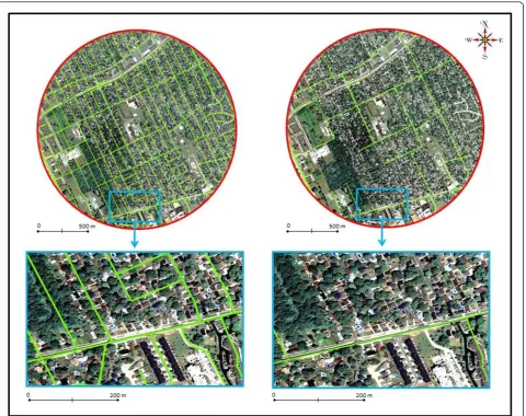
•In the main table of contents select“File”, navigate to the folder where the KML files were saved inStep 5 of Stage 1, and double click with the left mouse button on both files. These files were called “ Extra-cted_Roads”and“School_Buffer”in the example. •The road network and buffer layers should now appear in Google Earth. An illustration of these two layers for the example test site is shown in the top left panel of Figure 2.

Step 2: Deleting road segments without sidewalks

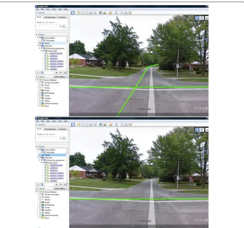
•On the“Places” table of contents click on the“+” button beside the name of the road network layer that was opened in Step 1("Extracted_Roads”in the example). This will open a list of the road segments that are located within the road shapefile buffer. • Double click with the left mouse button on the first road segment that appears in the list. This will take Google Earth to the location of the selected road, which will appear on the image in the main

part of the screen. An image of what this may look on a computer screen is shown in Figure 3.

•Visually inspect the segment to see if that road contains sidewalks on either or both sides. This pro-cess can be facilitated by zooming, panning or by using the street view option.

•If the road segment does not have a sidewalk on at least one side, delete that road segment by clicking on that road segment and selecting“delete”. If the road segment has a sidewalk on one or both sides, do nothing.

•Repeat Step 2for all the road segments in the sha-pefile buffer and delete all road segments that do not contain sidewalks. The top right panel in Figure 2 displays the road network pattern in the example buffer after all road segments without sidewalks have been deleted. Notice the differences between the green road network pattern in the top left and top right panels. These differences reflect the roads with-out sidewalks. See Figure 3 for an illustration of these differences.

Step 3: Save the modified road network (i.e., road seg-ments with sidewalks) as a Google Earth file.

•Select the road network layer in the“Places” table of contents (called “Extracted_Roads” in the exam-ple) and select “Save Place As”. In the example we called this new file“Roads_with_Sidewalks”.

Stage 3 - calculating the length of sidewalks along roads

Step 1

•Open ArcMap

• Select the“ET Geowizards Tool” icon (Note: you may need to install ET Geowizards. This program can be downloaded at http://www.ian-ko.com/. • In the pop-up-box select the “Import/Export” option from the left menu, and then the “Import from Google Earth”option.

•Select“Go”on the pop-up-box.

• In the new pop-up-box, in the “Select Google Earth file” text box, type in or select the Google Earth road network file that was saved inStep 5 of

Stage 2. This file was called “Roads_with_Sidewalks” in the example.

•In the“Specific output PDGB or folder”text box, specify the output folder.

•Select“Add layers to the Map”and then“Finish”. •Close the two pop-up-boxes.

Step 2: Provide the data frame with the proper map projection in order to accurately calculate the length of the roads with sidewalks.

• Select the data frame name (Layers) and choose “Properties”.

• In the pop-up-box select the“Predefined” folder, and within this folder select “Projected Coordinate Systems” then the “UTM” folder then the “NAD 1983” folder and then the appropriate Universal Transverse Mercator (UTM) geographic zone. Note that if you are calculating sidewalk distances outside of North America you should select “WGS 84” instead of “NAD 83”. In the example,“UTM NAD83

Zone 17 N”was selected as the sidewalks were being measured for a testing site that was located within this UTM zone. Sixteen different UTM zones were used in our national study of 315 Canadian schools. •Select“Apply” and then“OK”.

Step 3:

•In the pop-up-box select“Options” and then“Add field”.

•In the new pop-up-box type in a name for the new field. This new filed was called“Sidewalk_Length” in the example.

• Under“Type” select the“Double” option. For the “Field Properties” leave“Precision” as 0 and “Scale” as 0.

•Select“OK”.

Step 4: Calculate the distance of each road segment that has a sidewalk.

• In the pop-up-box select the new field that was created in Step 3 (this field was called“ Sidewalk_-Length” in the example) and then the “Calculate Geometry”option.

•Under“Property” select“Length”.

•Under“Coordinate System” select the“Use coordi-nate system of the data frame”option.

•Under“Units”select the unit of measure (e.g., kilo-meters, meters) you want the sidewalk distance to be measured in.

•Select“OK”.

Step 5:Calculate the distance of road segments con-taining sidewalks for the entire buffer.

•In the pop-up-box select the new field that was created in Step 3 (this field was called“ Sidewalk_-Length”in the example) and select“Statistics”. •Within the new pop-up-box the following statistics will be provided in a summary table: count (which is the number of road segments with a sidewalk in buf-fer), minimum (which is the length of the shortest road segment in the buffer that has a sidewalk), maximum (which is length of the longest road seg-ment in the buffer that has a sidewalk), sum (which is total length of road segments in the buffer that have a sidewalk), mean (which is the average length of road segments in the buffer that have a sidewalk), and standard deviation (which is standard deviation of the mean).

•An illustration of what the computer screen looked like at the end of Step 5for the example testing site is shown in Figure 4.

Step 6: Record sidewalk distance information

•Either manually record the data from the summary table or copy-and-paste it into another file type such as Excel.

Testing of method

The time required to obtain the sidewalk distance mea-sures within the 1 km circular buffer testing sites varied considerably. Some of the testing sites that were located in rural areas only contained a few roads and were com-pleted in approximately 5 minutes. Some of the testing sites that were located in metropolitan areas contained dense networks of roads and took over 30 minutes to complete.

Table 1 contains the median, interquartile range, mini-mum, and maximum values for the sidewalk distance measures that were obtained for the 315 testing sites where Google Street View data was available (note: Goo-gle Street View was not available for 121 of the total 436 school sampled for the HBSC). The distance of road segments with sidewalks in the testing sites ranged from 0 to 55.05 km, with a median of 16.20 km. When expressed relative to the distance of all road segments, the sidewalk coverage ranged from 0% to 100%, with a median of 52.8%. There were clear urban-rural gradients in these sidewalk measures such that the rural testing sites had shorter sidewalk distances and a smaller pro-portion of their roads had sidewalk coverage.

Discussion

The purpose of this technical advance was to present the protocol of a new GIS method for measuring the distance and coverage of sidewalks along roadways. The new sidewalk measurement protocol could be used in a variety of research, urban planning, and public health settings. The protocol could be used in descriptive research studies where sidewalk characteristics are being compared across different neighborhoods, communities, etc. It could be used in etiological research studies that aim to characterize the relationship between the pre-sence and length of sidewalks with walking behaviors. Municipalities that do not have geospatial sidewalk data could use this protocol to create such information. Pub-lic health and educational authorities could use the side-walk measures obtained in this protocol, in combination with road data, to identify safe routes for school-aged children to use when walking to school (i.e., all road segments used on travel route must have a sidewalk).

instances we navigated to the nearest intersection and did a 360 degree panoramic view to see if a view of the other side of the road was available, and if it was not, we zoomed out to the aerial view level. Third, in densely populated urban cores there were often trucks, buses, construction sites, etc. that blocked the view of the side of the road. In these instances we navigated forward or backward along the road at the street view level until we could see around the object(s), or if need be, zoomed out to the aerial view level.

The sidewalk measurement protocol developed in this study could be expanded in a number of ways. First, in addition to measuring the distance of sidewalks, it would be possible to measure the connectivity of side-walks, in a similar manner to how road (street)

connectivity measures are obtained. In fact, because 48% of the roads in the test sites of this national study did not have sidewalk coverage, it may be more appropriate to measure sidewalk connectivity rather than road con-nectivity in active transportation focused studies. The sidewalk connectivity measures could rely on the same type of indicators that are used to measure road connec-tivity such as the density of intersections per unit area, the percentage of intersections that are 3- or 4-way intersections, and the number of dead ends [7]. Researchers could take the sidewalk shapefiles saved at the end of Stage 2 in the protocol (i.e., road network that contains sidewalks) and obtain the connectivity measures on these files instead of the complete road network.

Figure 4Computer screen shot of the road network layer with sidewalk coverage for a 1 km radius circular buffer testing site obtained within ArcGIS and the summary table with the sidewalk length details (right side).

Table 1 Descriptive information on distance of sidewalks collected in the 1 km radius circular buffer testing sites across Canada

Testing Site Lowest 25th_{percentile 50}th_{percentile 75}th_{percentile Highest}

Sidewalks distance in 1 km buffer (km)

Total (N = 315) 0 8.06 16.20 28.61 55.05

Rural (N = 78) 0 1.84 4.24 10.40 26.14

Small cities (N = 116) 0 10.23 15.32 24.28 55.05

Metropolitan (N = 121) 0 20.63 27.73 33.76 51.53

Percentage of total road distance in 1 km buffer that had a sidewalk (%)*

Total (N = 315) 0 31.6 52.8 78.1 100

Rural (N = 78) 0 11.5 23.7 43.1 90.1

Small cities (N = 116) 0 39.9 52.8 73.2 98.3

Metropolitan (N = 121) 0 54.1 76.7 86.4 100

It may also be possible to integrate qualitative mea-surements of the sidewalks into the protocol, such as the sidewalk surface (e.g., pavement, asphalt, brick, etc.), sidewalk condition (e.g., excellent, in need of some repairs, in need of major repairs), and proximity of the sidewalks to the roads (e.g., directly beside road, boule-vard separating road and sidewalk). Thus, rather than measuring the distance of all sidewalks, these distance measures could be broken down by qualitative features (e.g., distance of sidewalks in poor, fair, and good condi-tion). Previous built environment research on parks has demonstrated that Google Earth can be used to obtain valid qualitative data [17]. It would be possible to inte-grate this type of information into Stage 2 of the side-walk measurement protocol. More specifically, each of the road segments with a sidewalk could be coded based on its qualitative features (i.e., rather than deleting a road segment; code it a different color based on its qua-litative features). Thus, in Stage 3 the distances of side-walks that meet different characteristics could be calculated.

A key advantage of the newly developed method is having the ability to measure sidewalk distances and coverage in a consistent manner in several different municipalities. This will allow researchers who are inter-ested in these types of studies to conduct regional, national, and even international studies. A key limitation of the newly developed method is that Google Earth does not provide street view and high resolution aerial images in all areas. In particular, these types of images are not available in many rural and remote areas. Another main limitation is the timing of when the Goo-gle Earth aerial and street view images were obtained relative to when the research study is completed. For example, in our city (Kingston, Ontario) the aerial images for Google Earth were obtained in 2004 and the street view images were obtained in 2009. If we were to conduct a Kingston-based study in 2012, some of the sidewalks in the city would have changed since 2004 and 2009, particularly in newly developed areas. Thus, as with most GIS measures of the built environment, the sidewalk measurement protocol would have a lim-ited utility in newly developed areas.

Conclusion

The measurement of built environment constructs is becoming an increasingly important component of public health research. This study provides a new measurement protocol that researchers can use to measure the distance and coverage of sidewalks along roadways. It is hoped that the use of this protocol in future studies will lead to an improved understanding of the walking environment and the determinants of walking in different areas.

Acknowledgements

This research was supported by grants from the Canadian Institutes of Health Research and the Heart and Stroke Foundation of Canada. IJ was supported by a Canada Research Chair award and an Early Researcher Award from the Ontario Ministry of Research and Innovation. The authors would like to thank Brandon Cheung for his assistance in obtaining the sidewalk measures.

Author details 1

School of Kinesiology and Health Studies, Queen’s University, 28 Division St., Kingston, ON, K7L 3N6, Canada.2_{Department of Community Health and} Epidemiology, Queen’s University, Kingston, Canada.

Authors_’contributions

AR developed the sidewalk measurement protocol, obtained the sidewalk measures for many of the testing sites, and revised the manuscript for important intellectual content. IJ came up with the study idea, was responsible for writing the manuscript, and completing the statistical analysis. Both authors approve the version that has been submitted.

Competing interests

The authors declare that they have no competing interests.

Received: 13 October 2011 Accepted: 29 March 2012 Published: 29 March 2012

References

1. Canada Fitness and Lifestyle Research Institute:2005 Physical Activity Monitor

Ottawa, ON: Canadian Fitness and Lifestyle Research Institute; 2006 [http:// www.cflri.ca/eng/statistics/surveys/pam2005.php].

2. Manson JE, Hu FB, Rich-Edwards JW, Colditz GA, Stampfer MJ, Willett WC, Speizer FE, Hennekens CH:A prospective study of walking as compared with vigorous exercise in the prevention of coronary heart disease in women.N Engl J Med1999,341(9):650-658.

3. Hu FB, Sigal RJ, Rich-Edwards JW, Colditz GA, Solomon CG, Willett WC, Speizer FE, Manson JE:Walking compared with vigorous physical activity and risk of type 2 diabetes in women: a prospective study.JAMA1999, 282(15):1433-1439.

4. Physical Activity Guidelines Advisory Committee:Physical Activity Guidelines Advisory Committee Report, 2008.Washington, DC: U.S. Department of Health and Human Services; 2008 [http://www.health.gov/ PAguidelines/Report/].

5. Frank LD, Sallis JF, Conway TL, Chapman JE, Saelens BE, Bachman W:Many pathways from land use to health: associations between neighborhood walkability and active transportation, body mass index, and air quality.J Am Plann Assoc2006,72(1):75-87.

6. Friedman MS, Powell KE, Hutwagner L, Graham LM, Teague WG:Impact of changes in transportation and commuting behaviors during the 1996 Summer Olympic Games in Atlanta on air quality and childhood asthma.JAMA2001,285(7):897-905.

7. Dill J:Measuring network connectivity for bicycling and walking.

Transport Research Board 2004 Annual Meeting (CD-ROM)Washington, D.C.; 2004.

8. Ewing R, Cervero R:Travel and the built environment - synthesis.

Transport Res Rec2001,1780:87-114.

9. Berrigan D, Pickle LW, Dill J:Associations between street connectivity and active transportation.Int J Health Geogr2010,9:20.

10. Owen N, Humpel N, Leslie E, Bauman A, Sallis JF:Understanding environmental influences on walking; Review and research agenda.Am J Prev Med2004,27(1):67-76.

11. Saelens BE, Sallis JF, Frank LD:Environmental correlates of walking and cycling: findings from the transportation, urban design, and planning literatures.Ann Behav Med2003,25(2):80-91.

12. Retting RA, Ferguson SA, McCartt AT:A review of evidence-based traffic engineering measures designed to reduce pedestrian-motor vehicle crashes.Am J Public Health2003,93(9):1456-1463.

14. Ewing R, Schroeer W, Greene W:School location and student travel: analysis of factors affecting mode choice.Transport Res Rec2004, 1895:55-63.

15. Lin J-J, Chang H-T:Built environment effects on children_’s school travel in Taipai: independence and travel mode.Urban Stud2010,47:867-889. 16. Boarnet MG, Anderson CL, Day K, McMillan T, Alfonzo M:Evaluation of the

California safe routes to school legislation: Urban form changes and children_’s active transportation to school.Am J Prev Med2005, 28(252):134-140.

17. Taylor BT, Fernado P, Bauman AE, Williamson A, Craig JC, Redman S: Measuring the quality of public open space using Google Earth.Am J Prev Med2011,40(2):105-112.

Pre-publication history

The pre-publication history for this paper can be accessed here: http://www.biomedcentral.com/1471-2288/12/39/prepub

doi:10.1186/1471-2288-12-39

Cite this article as:Janssen and Rosu:Measuring sidewalk distances

using Google Earth.BMC Medical Research Methodology201212:39.

Submit your next manuscript to BioMed Central and take full advantage of:

• Convenient online submission

• Thorough peer review

• No space constraints or color figure charges

• Immediate publication on acceptance

• Inclusion in PubMed, CAS, Scopus and Google Scholar

• Research which is freely available for redistribution