135 *Corresponding author
Email address: [email protected]
Optimizing turning operation of St37 steel using grey relational
analysis
S. Khalilpourazarya,*, P. M. Kashtibana and N. Payama
a
Department of Mechanical Engineering, Urmia University of Technology, Urmia, Iran
Article info: Abstract
Nowadays, in order to reach minimum production cost in machining operations, various optimization methods have been proposed. Since turning operation has different parameters affecting the workpiece quality, it was selected as a complicated manufacturing method in this paper. To reach sufficient quality, all influencing parameters such as cutting speed, federate, depth of cut and tool rake angle were selected as input parameters. Furthermore, both surface roughness and tool life were considered as the objectives. Also, ST37 steel and M1 high speed steel (HSS) were selected as workpiece material and tool, respectively. Subsequently, grey relational analysis was performed to elicit optimal values for the mentioned input data. To achieve this goal, first, degree of freedom was calculated for the system and the same experiments were performed based on the target values and number of considered levels, leading to calculating grey relational generating, grey relational coefficient and grey relational grade. As the next step, the grey relational graph was sketched for each level. Finally, optimum values of the parameters were obtained for better surface roughness and tool life. It was shown that the presented method in the turning operation of ST37 led to high surface quality and tool life.
Received: 26/09/2012 Accepted: 28/08/2013
Online: 03/03/2014
Keywords: Turning, Optimization, Grey analysis, Sourface roughness, Tool life.
1. Introduction
Material removal from rotating wokpiece by applying forces is known as turning operation [1]. In turning operation, significant controllable parameters on the surface roughness and tool wear can be listed as follows: tool geometry, cooling system, depth of cut, spindle rotational speed, cutting speed, cutting tool geometry and federate [1]. There are also uncontrollable parameters such as
ambient temperature, machine age and type of used material. Due to the constraints of full elimination of effects of uncontrollable parameters and their negligible effectiveness, optimization is taken into consideration for controllable parameters in order to obtain more efficient parameters [1].
136
Since turning operation has different parameters affecting the workpiece quality and tool wear, it was selected as a complicated manufacturing method in this paper. Optimization of turning parameters by Taguchi method was reported in 1998 [2]. Sori et al. utilized micro-genetic algorithm method for optimizing the turning operation. Surface roughness and tool wear were selected as output parameters [3]. Davim investigated optimization of turning parameters through the orthogonal arrays [4].
A plan of experiments based on Taguchi technique was performed on machining with the cutting conditions prefixed in workpieces. An orthogonal array and analysis of variance were employed to investigate cutting characteristics of MMC (A356/20/SiCp-T6) using PCD cutting tools[4]. The objective was to optimize tool wear, power consumption of machining operation and surface roughness in the workpiece. To have sufficient quality, all influencing parameters such as cutting velocity, fedrate and cutting time were selected as input parameters. Lin used a combination of Taguchi method and grey relational analysis for optimization of the turning operation [5]. Mana and Bhattacharyya studied machining conditions of Al/Sic alloy in order to reach minimum surface roughness [6].
The corresponding L27 orthogonal array was selected prior to investigating degree of freedom for the system and number of levels for the tests. Also,Analysis of Variance was utilized to optimize height of surface roughness Ra andRt. Nalbat et al. utilized Taguchi method in order to minimize surface roughness values in turning operation [7]. Golkarpoor et al. studied cutting forces, cutting temperature and surface roughness as input parameters in turning operation of St37 steel in order to determine tool life cycle [8]. Mahdavinezhad et al. considered effect of cutting speed on the tool wear ratio and material removal rate in the turning operation of St37 steel.
Turning operation was performed in two conditions of with and without lubricant [9]. Using grey analysis, the problem with multiple
objectives was changed to the problem with one objective which led to easier data analyses and inferences. Due to different restrictions and amounts associated with optimization parameters, a rather challenging comparison is expected. Hence, normalization is necessary to accomplish a valid comparison between the parameters. After normalizing the data, which was done in the stage of generating grey relational to obtain grey relational coefficient and grey relational grade, the final decision from plotted grey graph can be made. In this work, due to high effect of the cutting tool angles on the turning operation, the tool rake angle was studied using grey method for the first time. Furthermore, in order to determine effect percentage of the parameters in the optimum condition as well as effect of input parameters on the output ones, some new equations were recommended.
The ultimate goal of the current paper was to investigate simultaneous effects of different turning parameters on surface roughness of the manufactured St37 steel workpieces as well as high steel speed (HSS) cutting tool wear. Here, the grey method was selected to extract optimal values of the cutting speed, depth of cut, federate and tool rake angle that led to the minimum surface roughness and tool wear. First, degrees of freedom of the system were calculated. Then, based on these data and the number of levels, the corresponding orthogonal arrays were obtained for the tests. After the grey relational coefficient and grade were calculated, grey relational graph was depicted.
137 were elicited after grey relational analysis was
verified by the experimental tests.
2. Experimental setup
The workpiece used in this study had effective length of 400 mm and diameter of 45 mm [3]. Chemical composition (weight percent) of St37 steel is given in Table 1 [10].
Table 1. Chemical composition of the St37 steel
[10].
Element Weight %
C 0.09-0.15 Mn 0.35-0.65 Si 0.17-0.35 S (Max) 0.040 P (Max) 0.040 Cr (Max) 0.30 Ni (Max) 0.30 Cu (Max) 0.30
Also, orthogonal cutting was done by high speed steel tool with clearance angle of
6
. M1 is a high speed steel in Molybdenum series. Table 2 lists equivalents of this steel in different standards.Table 2. Equivalents of M1 high speed steel in
different standards.
Standard Steel name
DIN DIN 1.3346
BS BM 1
AISI M1
M1 has good red-hardness, high wear resistance and cutting ability. After heat treatment, its hardness can reach 63-65 HRC. Chemical composition (weight percent) of M1 high speed steel is given in Table 3 [11].
Table 3. Chemical composition of the M1 high
speed steel [11].
Element Weight %
C 0.8
W 1.5
Mo 8
Cr 4
V 1
To increase life of high speed steel, tools are sometimes coated. One such coating is TiN. Titanium nitride is a golden colour ceramic with coating applied by physical vapor deposition (PVD). High hardness combined with low friction properties ensures considerably longer life for tool or alternatively better cutting performance from tools which have not been coated. TiN coating is mainly used in drills and taps. Thickness of TiN coating layer over the surface of tool is about 500 µm [11]. Figure 1 shows geometry of the cutting tool and related parameters and Table 4 demonstrates the amount of these parameters [12].
Fig. 1. Geometry of cutting tool.
Table 4. Amount of tool parameters [12].
Specification Dimension(in mm)
ISO Standard d t r SNGN 120708 12.7 7.94 0.8
Tool holder was selected according to the ISO standard in the CSRNR 2525 M12-4 type. Figure 2 depicts geometry of the holder and Table 5 lists values for these parameters [12].
Fig. 2. Tool's geometrical parameters [12].
138
Table 5. Amount of tool holder parameters [12].
Designation Dimension(mm)
CSRNR/L 2525M12-4
1
f l1 l3 b h
27 150 34.3 25 25
The lathe machine model used here was D TN50 manufactured in the Machine Sazi plant, Iran. In order to increase accuracy, a new insert of tool was used for each test. The spindle speed was obtained via KIMO Tachometer CT100. In this paper, tool life was defined as the volume of the workpiece that had to be removed in order to reach a special (the 1.5 times) enhancement of the surface quality. Then, calculation of this volume was done in the inverted value that helped to have better and more adequate selections according to Eq. (1.1) [3, 13].
3
10
1
1
L
d
D
v
(1.1)where
v
is removed volume, D is diameter of the workpiece, d is depth of cut and L is workpiece length, surface quality of which increases 1.5 times by machining. Furthermore, the spindle speed was calculated by Eq. (1.2) in all the work steps [14].D
V
N
1000
(1.2)where V is cutting speed in m/s, D is workpiece diameter in mm and N represents frequency of revolution in rev/min. The roughness tester was portable (model MarSurf
TS1) with the capacity to
measure
R
max,RzandR
a for different surfaces and was manufactured in Mahr plant, Germany. Prob of the roughness tester moved on the work piece surface and the data were sent to a computer. When the data were put in the computer, the surface roughness profile was drawn and values of itsR
aroughness were determined. Evaluation or cut off length for the manufactured work piece was equal to 7 mm according to the ISO 4288 standard. Figure 3 demonstrates the roughness tester (model MarSurf TS1).Fig. 3. The roughness tester model MarSurf TS1.
3. Levels of the experiment
Grey analysis method was introduced for the first time by J. Deng in 1982 [15]. Unlike difficulties and infeasibility of other methods, this method can be applied for the systems with multiple objectives [16]. In grey analysis, each test has input parameters divided to levels according to the application conditions or effectiveness. In this paper, the experiments were performed for the first three parameters (i.e. cutting speed, federate and depth of cut) at three different levels and for the tool rake angle at two different levels (see Table 6).
Table 6. Parameters and related levels [3].
Parameters Test levels
1 2 3
Cutting speed(m/min) 17 25 33 Federate (mm/rev) 0.09 0.13 0.17 Depth of cut (mm) 0.2 0.4 0.6 Rake angle (Degree) 0 14
In the next step, the machine set up was done via all the data provided in Table 6.
4. Orthogonal array
139 (3.1)
FD =1+( degree of freedom×level),
Then, the obtained value for degree of freedom is: 8 ) 1 2 2 2 (
1
FD
Since degree of freedom for this system is 8, the array L18can be used due to capability of the array in designing specific type of the experiment. Table 7 shows the obtained values of the surface roughness and tool wear for each run using Eq (1.1) and roughness tester (model MarSurf TS1). It is worth noting that setup of different tests should be run in a non-repeating fashion and that setup of each test should be done at three times for the purpose of increasing accuracy and decreasing various types of errors.
Table 7. Experimental layouts using orthogonal
array and measured results [3].
Run
Orthogonal array Test results
F ed er at e (m /m in) C ut ting s pe ed (m m /r ev) D ept h o f c u t (m m ) R ake a ng le (D eg re e) S ur fa ce roug hne ss (µ m ) T ool li fe
1 1 1 1 1 6.53 41.176 2 1 2 2 1 7.15 37.703 3 1 3 3 1 8.1 35.295 4 2 1 1 1 7.21 44.539 5 2 2 2 1 7.05 33.087 6 2 3 3 1 6.81 29.277 7 3 1 2 1 5.79 48.179 8 3 2 3 1 6.02 43.096 9 3 3 1 1 5.71 36.868 10 1 1 3 2 5.53 53.57 11 1 2 1 2 5.49 20.607 12 1 3 2 2 6.02 75.449 13 2 1 2 2 3.21 45.714 14 2 2 3 2 4.1 37.7 15 2 3 1 2 3.55 55.698 16 3 1 3 2 2.48 70.872 17 3 2 1 2 2.25 81.907 18 3 3 2 2 2.54 61.977
5. Generating grey relational
Normalization is necessary to achieve valid comparison between the parameters. Eqs. (5.1-3) introduce relations of different possibilities with the normalization process. If target value of original sequence is infinite, a characteristic of ‘‘the-larger-the-better’’ can be expected. The original sequence can be normalized as follows [17]: (5.1) , ) ( min ) ( max ) ( min ) ( 1 ) ( 0 0 0 0 * k X k X k X k X k X i i i i i
Since smaller values are desirable, the original sequence can be normalized as follows:
(5.2)
,
)
(
min
)
(
max
)
(
)
(
max
1
)
(
0 0 0 0 *k
X
k
X
k
X
k
X
k
X
i i i i i
In case there is a definite target value to be achieved, the original sequence can be normalized as follows:
(5.3)
,
)
(
max
)
(
1
)
(
0 0 0 0 *X
k
X
X
k
X
k
X
i i i
where, Xi*(k)is the value after grey relational generation (data pre-processing),
) (
max Xi0 k is the largest value ofXi0(k),
) (
minXi0 k is the smallest value of Xi0(k) and X0 is the desirable value [17, 18].
) (
*
k
Xi is the result of grey analysis for the ith response in the kth test while
)
(
k
140
6. Grey relational coefficient
Grey relational coefficient has a value between zero and one and indicates the distance from ideal value. Grey relational coefficient is calculated using the following formula [19, 20]: (6.1)
,
.
)
(
.
)
(
max 0 max min
k
k
i iwhereminrepresents minimum deviation of data values,
maxis maximum deviation of data values,
0i(
k
)
shows deviation value for the reference data and
i(
k
)
is grey coefficient. Each parameter in Eq. (6.1) is separately calculated using the following equations [20]: (6.2),
)
(
)
(
)
(
0* *0i
k
X
k
X
ik
(6.3),
)
(
)
(
max
max
0* *max
X
k
X
ik
(6.4),
)
(
)
(
min
min
0* *min
X
k
X
ik
It should be noticed that value of the grey coefficient is restricted to the range [0, 1] and, according to [21], optimal grey coefficients are usually selected as average (0.5).
7. Grey relational grade
Grey relational grade is a parameter obtained after grey relational coefficient. This parameter is determined using Eqs. (7.1-2) when effects of all parameters are assumed to be equal as follows [22, 23]:
(7.1)
,
)
(
1
1
mk i i
i
k
m
(7.2),
1
1
m i i
where
iis weighted value or importance of each parameter. When all the parameters have the same level of effectiveness,
ican be neglected. Also,
ijis the grey relational coefficient and
i is grey relational grade. Table 8 lists the related grey relational grade for each grey relational coefficient.Table 8. Grey relational coefficient and grey
relational grade.
Grey relational
grade Grey relational coefficient
Run Tool
life Surface
roughness
(
µm
)
0.418 0.429 0.406 1 0.392 0.409 0.374 2 0.365 0.397 0.333 3 0.411 0.451 0.371 4 0.382 0.386 0.379 5 0.379 0.368 0.391 6 0.464 0.476 0.452 7 0.439 0.441 0.437 8 0.432 0.405 0.458 9 0.496 0.520 0.471 10 0.404 0.333 0.474 11 0.631 0.826 0.437 12 0.606 0.459 0.753 13 0.511 0.409 0.613 14 0.616 0.539 0.692 15 0.831 0.735 0.927 16 1.000 1.000 1.000 17 0.758 0.606 0.910 18
8. Grey relational grade for each level
Eqs. (8.1-2) can be used to determine grey relational grade for each level. It is obvious that grey relational grade for each level is the average amount of all grades [23]:
(8.1)
,
1
1
k i ik
A
(8.2),
n
m
k
141 number of tests and n is the number of levels.
Table 9 represents a column listing Max-Min values for the grey grade data obtained from the maximum and minimum values of grey grade for each level. These values indicate robustness of each parameter. When it is high for a parameter, the corresponding parameter is unstable and vice versa [24, 25].
Table 9. Grey relational grade for each level.
Parameters Levels Max-Min
1 2 3
Cutting speed
(m/min) 0.451 0.484 0.654 0.203 Federate
(mm/rev) 0.538 0.521 0.530 0.016 Depth of cut
(mm) 0.547 0.539 0.504 0.043 Rake angle
(Degree) 0.409 0.650 0.241
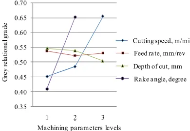
9. Grey relational graph
Grey Relational Graph is the graph of the table containing levels and grey relational grade for each level. This graph is easily drawn by connecting the table points to each other. In this study, grey graph for each level is drawn according to the obtained tables. We also integrated all four graphs into one for better comparison (see Fig. 4).The amount of the slope in Fig. 4 indicates the sensitivity of that the parameter (e.g.as slope decreases, the effectiveness of the parameter decreases as well).
0.35 0.40 0.45 0.50 0.55 0.60 0.65 0.70
1 2 3
يﺮ
ﮔ ﻪ
ﺟر
د
ﺶﯾﺎﻣزآ حﻮﻄﺳ
ﯽﺷﺮﺑ ﺖﻋﺮﺳ يوﺮﺸﯿﭘ ﺖﻋﺮﺳ شﺮﺑ ﻖﻤﻋ شﺮﺑ ﻪﯾواز
Cutting speed, m/min
Feed ra te, mm/rev
Rake a ngle, degree
Machining pa rameters levels
G
re
y
r
e
la
ti
o
n
a
l g
ra
d
e
Depth of cut, mm
Fig. 4. Effect of machining parameter levels on the
multi-performance.
10. Parameters effectiveness for when optimum condition occurs
The effectiveness of each parameter on test results is exploited by Eq. (10.1) and general optimum condition is calculated by Eq. (10.2).
(10.1)
,
100
1
m
i ij ij i
A
N
A
N
(10.2)
),
( ij ij
ij Max Min A
N
where,
ishows the ith parameter effectiveness with jth level in percent andN
A
ij indicates the Max-Min value of grey relational degree for each level. The effectiveness values of internal parameters are listed in Table 10.Table 10. Percentage of parameters influence in
optimum condition.
Optimum parameter influence in percent Parameters
40.33 Cutting Speed(m/min)
3.22 Federate (mm/rev)
8.55 Depth of Cut (mm)
47.89 Rake angle (Degree)
11. Effectiveness value of each parameter
Calculating influence of each parameter can be done by Eqs. (11.1-4).
(11.1)
,
1
1
ki ij
K
B
(11.2)
,
n
m
k
(11.3)
,
100
1
m
i ij ij i
B
N
B
N
B
(11.4)
),
( ij ij
ij Max Min B
N
142
coefficient, m is the number of tests with level value of n, Bi is the ith parameter's effectiveness percent for jth level and
N
B
ijis the Max-Min value of grey relational coefficient for each level. Table 11 lists effectiveness values of internal parameters on the results.Table 11. Effectiveness values of internal
parameters.
Parameters Tool life %
Surface quality %
Cutting speed(m/min) 40.24 43.72 Federate (mm/rev) 6.18 4.13 Depth of cut (mm) 11.14 5.95 Rake angle (Degree) 42.45 46.20
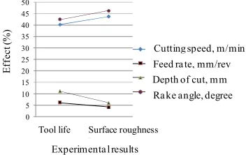
12. Parameters' effectiveness graph
This graph is drawn by the data obtained from Table 11. The graph for each parameter is drawn and, as shown in Fig. 5, all four graphs are integrated into one (see Fig. 5).
0 5 10 15 20 25 30 35 40 45 50
راﺰﺑا ﺮﻤﻋ ﺢﻄﺳ ﺖﯿﻔﯿﮐ
ﺪ
ﺻر
د
ﺮﯿ
ﺛﺄﺗ
تﺎﺸﯾﺎﻣزآ ﺞﯾﺎﺘﻧ
ﯽﺷﺮﺑ ﺖﻋﺮﺳ يوﺮﺸﯿﭘ ﺖﻋﺮﺳ شﺮﺑ ﻖﻤﻋ شﺮﺑ ﻪﯾواز
Cutting speed, m/min Feed ra te, mm/rev Depth of cut, m m Ra ke angle, degree
Surface roughness Tool life
Experimenta l results
E
ff
ec
t (
%
)
Fig. 5. Effectiveness of internal parameters.
13. Results and discussion
It can be concluded from Table 8 that the test number 17 had a higher grey degree when compared with other tests and was closer to the test number 1, which can be evidence for the ideal form of grey relational grade. So, the 17th setup was the optimum one for the level arrangement and led to the best results while the third one was the worst. According to Table 9, it can be inferred that tool rake angle was unstable due to rather high amount of the Max-Min values and federate was stable since the related Max-Min was low, implying that variance of the tool rake angle was important
and had the highest effect on test results whereas the federate had the least effect on the results. The results for presented the optimum condition were compared with the optimum test values obtained from the manufactured work pieces (i.e. minimum surface roughness and maximum tool wear), as shown in Table 12. Optimal test values were obtained according to the values presented in Tables 6 and 7 and surface roughness quantities of the manufactured work pieces.
Table 12. Optimum values for all input parameters.
Parameters Optimum condition
Optimum test
Cutting speed (m/min) 33 33 Federate (mm/rev) 0.09 0.13 Depth of cut (mm) 0.2 0.2 Rake angle (Degree) 14 14
Also, the weakest results for the surface quality and tool life are summarized in Table 13.
Table 13. The worst values of parameters.
Parameters Weakest condition
Weakest test response
Cutting speed (m/min) 17 17 Federate (mm/rev) 0.13 0.17 Depth of cut (mm) 0.6 0.6 Rake angle (Degree) 0 0
In this study, results obtained by the grey relational method showed that:
1- According to the grey graph in Fig. 4, when the cutting speed was enhanced from 17 m/min to 33 m/min, test results and objectives improved.
2- Increasing depth of cut from 0.2 mm to 0.6 mm led to poor results.
3- Increasing the tool rake angle from 0 to 14 degree gave appropriate and better results. 4- Test results were deteriorated when the federate increased from 0.09 mm/rev to 0.13 mm/rev while this trend completely changed from 0.13 mm/rev to 0.17 mm/rev and the results were improved.
143 federate with the value of 3.22% had the
maximum and minimum effectiveness for general conditions of the test, respectively. 6- According to the data listed in Table 11, the tool rake angle had superior influence on surface roughness (46.2%) while federate had the least effect on the surface roughness (4.13%).
7- Data in Table 11 reported the same issue mentioned in 6. Influence of the rake angle was 42.45% and that of the federate was 6.18%, indicating the highest and lowest effects on tool life, respectively.
8- From Fig. 5, it can be concluded that the tool rake angle and cutting speed had higher influence on objectives than depth of cut and federate.
9- After grey relational analysis was accomplished, optimal value of each input parameter was compared with its counterpart obtained from the experimental tests (see Table 12). Optimum test parameters were identified from the measurement of surface roughness using MarSurf TS1roughness tester and the tool life was calculated using Eq. (1.1).
14. Conclusions
In this study, cutting speed, federate, depth of cut and tool rake angle were considered as internal parameters for optimizing ST37 steel turning process by grey relational analysis. Also, the correspondingL18orthogonal array was selected prior to investigating degree of freedom for the system and the number of levels for the tests. Following grey relational generation and calculating grey relational coefficient and grade, grey graph was drawn based on the grey grade for each level. Finally, using the grey graph, the optimal amount of each parameter was exploited for better surface roughness and tool life. Since tool rake angle and federate had the maximum and minimum effects on the surface roughness and tool life, respectively, it was shown that performance characteristics of the turning process of ST37 improved using the method recommended by this study.
Acknowledgement
This research project was carried out under technical support of the Orumieh Tractor Manufacturing Company (O.T.M.Co).
References
[1] F. Klocke, Manufacturing Processes 1: Cutting, First ed., Springer, New York, pp. 110-134, (2011).
[2] B. C. Routara, B. K. Nanda, A. K. Sahoo, D. N. Thatoi and B. B. Nayak, “Optimization of multiple performance characteristics in abrasive jet machining using grey relational analysis”, Int. J. Manufact. Technol. Manag., Vol. 24, No. 2, pp. 4-22, (2011).
[3] E. Sori, R. Narimani and E. Rohanie esfhani, “Optimization turning parameters using micro genetic algorithm”, Proc. of 5th National Manufacturing Conference, Najafabad, Iran, pp. 141-146, (2007).
[4] J. P. Davim, “Design of optimization of cutting parameters for turning metal matrix composites based on the orthogonal arrays”, J. Mater. Process. Technol., Vol. 132, No.1, pp. 340-344, (2003).
[5] C. L. Lin, “Use of the taguchi method and grey relational analysis to optimize turning operations with multiple performance characteristics”, Mater. Manufact. Process., Vol. 19, No. 2, pp. 209-220, (2004).
[6] A. Manna and B. Bhattacharyya, “Investigation for optimal parametric combination for achieving better surface finish during turning of Al/SiC-MMC”,
Int. J. Adv. Manufact. Technol., Vol. 23, No. (9-10), pp. 658-665, (2004).
[7] M. Nalbant, H. Gokkaya and G. Sur, “Application of taguchi method in the optimization of cutting parameters for surface roughness in turning”, Mater. Des., Vol. 28, No. 4, pp. 1379-1385, (2007).
144
surface and temperature on the tool life in turning operation of St37 steel”, Proc. of
1
th NationalMechanic
Conference, Majlesi, Iran, pp. 100-106, (2007). [9] R. Mahdavinezhad, M. Khajeh Afzaliand E. Daziani, “Analysis of tool wear in turning operation of St37 steel”, J. Appl. Mech., Vol. 45, No. 3, pp. 77-85, (2011).
[10] M. Kutz, Handbook of Materials Selection, 2nd ed., John Wiley & Sons, Inc., New York, pp. 50-72, (2002). [11] M. Boccalini and H. Goldenstein,
“Solidification of high speed steels”, Int. Mater. Rev., Vol. 46, No. 2, pp.92-115, (2001).
[12] Taegu Technology Company, Cutting Tools Catalogue, Korea Industry, Seoul, pp. 310-315, (2001).
[13] ASM handbook, Metals Handbook: Surface Engineering, First ed., New York, pp. 230-312, (1994).
[14] E. Isakov, Cutting Data for Turning of Steel, First ed., Industrial Press Inc., New York, pp. 102-150, (2009).
[15] A. Sharma and V. Yadava, “Optimization of cut quality characteristics during Nd: YAG laser straight cutting of Ni-Based superalloy thin sheet using grey relational analysis with entropy measurement”, Mater. Manufact. Process., Vol. 26, No. 12, pp. 1522-1529, (2011).
[16] B. Naveen, A. Kumar, S. Maheshwari and C. Sharma, “Optimization of electrical discharge machining process with Cu-W powder metallurgy electrode using grey relation theory”, Int. J. Mach. Mach. Mater., Vol. 9, No. 2, pp. 103-115, (2011).
[17] U. Caydas and A. Hascalik, “Use of the grey relational analysis to determine optimum laser cutting parameters with multi-performance characteristics”,
Optics & Laser Technol., Vol. 40, No. 7, pp. 987-994, (2008).
[18] D. K. Panda, “Modelling and optimization of multiple process attributes of electro discharge machining process by using a new hybrid approach
of neuro–grey modeling”, Mater. Manufact. Process, Vol. 25, No. 6, pp. 450-461, (2010).
[19] C. J. Tzeng, Y. H. Lin, Y. K. Yan and M. C. Jeng, “Optimization of turning operations with multipleperformance characteristics using the taguchi methodand grey relational analysis”,
J.Mater. Process. Technol., Vol. 209, No. 6, pp. 2753-2759, (2009).
[20] S. Khalilpourazary and P. Nasib, “Optimization of the tool wear, machining rate and overcut of metallic composite Al-4Cu-6Si-10wt%SiCP in EDM drilling operation”, Proc.of 21th Annual International Conference on Mechanical Engineering (ISME2013),
Tehran, Iran, pp.10-17, (2013).
[21] K. Palanikumara, B. Lathab, V. S. Senthilkumarc and J. Paulo, “Analysis on drilling of glass fiber–reinforced polymer (GFRP) composites using grey relational analysis”, Mater. Manufact. Process., Vol. 27, No. 3, pp. 297-305, (2012).
[22] J. A. Barriosa, A. Cavazosa, L. Leducb and J. Ramírezb, “Fuzzy and fuzzy grey-box modelling for entry temperature prediction in a hot strip mill”, Mater. Manufact. Process., Vol. 26, No.1, pp. 66-77, (2011).
[23] S. Khalilpourazary, P. Nasib and M. Mohammady, “Optimization of the surface roughness and machining rate of metallic composite Al/Sic in EDM machining using grey relational method”, Proc. Of 1th National Manufacturing Conference, Malayer, Iran, pp. 80-86, (2013).
[24] J. Kopac and P. Krajnik, “Robust design of flank milling parameters based on grey-taguchi method”, J. Mater. Process. Technol., Vol. 191, No. (1-3), pp. 400-403, (2007).
[25] S. Datta, A. Bandyopadhyay and P. K. Pal, “Grey-based taguchi method for optimization of bead geometry in submerged arc bead-on-plate welding”,
![Fig. 2. Tool's geometrical parameters [12].](https://thumb-us.123doks.com/thumbv2/123dok_us/9969889.1985309/3.595.366.502.535.676/fig-tool-s-geometrical-parameters.webp)
![Table 5. Amount of tool holder parameters [12].](https://thumb-us.123doks.com/thumbv2/123dok_us/9969889.1985309/4.595.349.463.85.217/table-tool-holder-parameters.webp)
![Table 7. Experimental layouts using orthogonal array and measured results [3].](https://thumb-us.123doks.com/thumbv2/123dok_us/9969889.1985309/5.595.90.291.340.704/table-experimental-layouts-using-orthogonal-array-measured-results.webp)