R E S E A R C H A R T I C L E
Open Access
Finite increment calculus (FIC):
a framework for deriving enhanced
computational methods in mechanics
Oñate Eugenio
**Correspondence:
[email protected] Centre Internacional de Metodes Numerics en Enginyeria - CIMNE, Gran Capitán s/n, Campus Nord UPC, 08034 Barcelona, Spain
Abstract
In this paper we present an overview of the possibilities of the finite increment calculus (FIC) approach for deriving computational methods in mechanics with improved numerical properties for stability and accuracy. The basic concepts of the FIC procedure are presented in its application to problems of advection-diffusion-reaction, fluid mechanics and fluid-structure interaction solved with the finite element method (FEM). Examples of the good features of the FIC/FEM technique for solving some of these problems are given. A brief outline of the possibilities of the FIC/FEM approach for error estimation and mesh adaptivity is given.
Keywords: Finite increment calculus, Finite calculus, FIC, Finite element method, Computational mechanics
Background
The finite increment calculus (FIC) (sometimes called finite calculus, in short) was pro-posed by Oñate [1] as a conceptual framework for deriving stabilized numerical methods [mainly the finite element method (FEM)] for solving advective–diffusive transport and fluid compressible flow problems in mechanics for situations where numerical methods typically fail (i.e., high Peclet/Reynolds numbers and incompressible situations) [2,3].
The essence of the FIC approach lays in solving the governing differential equations in mechanicswritten in a modified form, using any discretization method such as the Galerkin finite element (FE) method, any standard finite difference (FD) scheme, the finite volume (FV) method, meshless methods, etc. The FIC modified governing equations are obtained bywriting the equations for balance of heat, momentum and mass in a space-time domain of finite incremental size, and not in a domain of infinitesimal size, as it is usually done.
Accounting for the finiteness of the balance space-time domain introduces naturally additional terms in the classical differential equations of continuum mechanics, which now become a function of the balance domain dimensions. The merit of the modified governing equations derived via FIC is thatthey are a natural starting point for deriving stabilized numerical schemes. Moreover, the different stabilized FE, FD and FV methods typically used in practice can berecoveredusing FIC.
©Eugenio 2016. This article is distributed under the terms of the Creative Commons Attribution 4.0 International License (http:// creativecommons.org/licenses/by/4.0/), which permits unrestricted use, distribution, and reproduction in any medium, provided you give appropriate credit to the original author(s) and the source, provide a link to the Creative Commons license, and indicate if changes were made.
The FIC technique has been used in conjunction with the finite element method (FEM) for deriving stabilized FIC/FEM procedures for a wide range of problems in advective– diffusive-reactive transport, fluid mechanics, incompressible solids and fluid-structure interaction (FSI) situations, among others [1,4–28]. The FIC approach has also been used in conjunction with the meshlessfinite point methodfor solving some of these problems [13,29–31].
The layout of the paper is the following. In the next section the main concepts of the FIC method are introduced. Details of the FIC approach for advection–diffusion-reaction problems solved with the FEM are presented. Then the possibilities of the FIC/FEM technique in fluid and solid mechanics and FSI problems solved with the particle finite element method (PFEM) are outlined. Examples of applications are given for some of the problems considered. Finally, a brief outline of the possibilities of the FIC/FEM approach for error estimation and mesh adaptivity is given.
Basic ideas of the FIC approach
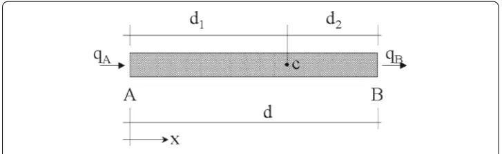
Let us consider a steady-state advection–diffusion problem in a 1D domainof length L. The equation of balance of fluxes in a subdomain of sizedbelonging to(Fig.1) is written as
qA−qB=0 (1)
whereqAandqBare the incoming and outgoing fluxes at pointsAandB, respectively. The fluxqincludes both the advective and diffusive terms; i.e.,q=ρcvφ−kddxφ, whereφis the transported variable (i.e., the temperature in a thermal problem),vis the velocityρ, cand kthe density, the specific flux parameter and the diffusitivity of the material, respectively. Let us express now the fluxesqAandqB in terms of the flux at an arbitrary pointC within the balance domain (Fig.1). ExpandingqAandqBin Taylor series around pointC up to second order terms gives
qA=qC −d1
dq dx|C +
d12 2
d2q
dx2|C+O(d 3
1), qB=qC +d2
dq dx|C +
d22 2
d2q
dx2|C+O(d 3 2)
(2)
Substituting Eq. (2) into Eq. (1) gives after simplification and neglecting higher order terms
dq dx −
h 2
d2q
dx2 =0 (3)
whereh=d1−d2and all the derivatives are computed at the arbitrary pointC.
Standard calculus theory assumes that the balance domain d is of infinitesimal size. Hence, the underlined term in Eq. (3) can be neglected and the resulting flux balance equation is simplydqdx =0. In FIC we will relax this assumption and allow the space balance domain to have afinite size. The new balance Eq. (3) incorporates the underlined term which introduces thecharacteristic length h. Obviously, accounting for higher order terms in the Taylor expansions of Eq. (2) would lead to additional terms in Eq. (3) incorporating higher powers ofh.
Distancehin Eq. (3) can be interpreted as a free parameter depending on the location of pointC within the balance domain. Note that−d ≤ h ≤ dand, hence,hcan take a negative value. At the discrete solution level the domaindshould be replaced by the balance domain around a node. This gives for an equal size discretization−le ≤h≤le whereleis the element or cell dimension. The fact that Eq. (3) is theexact flux balance equation(up to second order terms) for any 1D domain of finite size and that the position of pointCis arbitrary, can be used to derive numerical schemes with enhanced properties. This goal can be reached by computing the characteristic length parameterhusing an adequate “optimality” condition; for instance, in the FEM context we can look for the elemental or nodal value of hthat ensures a prescribed (small) error in the numerical solution [1,10,32]. In some cases, the optimal value ofhfor each element leading to an exact nodal solution can be found [1,6,21,28,32].
Applications to the 1D convection–diffusion problems
Consider, for instance, Eq. (3) applied to the 1D advection–diffusion problem in a 1D domain of lengthL. Neglecting the third order derivatives, Eq. (3) can be rewritten in terms ofφas
−vdφ dx +
k+ ρcvh 2
d2φ
dx2 =0; 0≤x≤L (4)
We see that the FIC method introduces naturally an additional diffusion term in the standard advection–diffusion equation. This is the basis of the popular “artificial diffusion” procedure [1–3] where the characteristic lengthhis expressed as a function of the cell or element dimension. The criticalvalue of hcan be computed by ensuring that the solution has a physically meaning (i.e.,φi≥0 for the Dirichlet problem with non negative prescribed values ofφ atx = 0 andx = L). For an equal size FEM discretization this gives h ≥
1−γ1
le, whereγ = ρcvl2ke is the element Peclet number. The inequality applies for γ > 0 and it should be reversed for γ < 0. Also his taken to be zero for |γ|<1. Theoptimalvalue ofhfor all the elements leading to exact nodal values can also be found for this simple case ash=cothγ −γ1le[1–3]. The same results are obtained using the FD method with a central difference scheme, whereleis now the cell dimension [1,3].
Equation (3) can be extended to account for source terms. The FIC governing equation can then be written in compact form as
r− h 2
dr
dx =0; r:=ρcv dφ
dx − d dx
kdφ
dx
−Q (5)
Boundary conditions
The FIC governing equations are completed with the standard Dirichlet condition pre-scribing the value ofφat the boundaryφ(i.e.,φ =φp=0 atφ).
For consistency a FIC form of the Neumann boundary condition should be used. This can be obtained by invoking balance of fluxes in a domain of finite size next to the boundary q. The FIC Neumann boundary condition when the external (diffusive) flux is prescribed to a valueqpis [1]
kdφ dx +q
p+h
2r=0 atq (6)
Note that forh=0 the standard Neumann boundary condition for prescribed diffusive flux is obtained.
We emphasize that the relevant feature of the FIC procedure is that the underlined terms in Eqs. (5) and (6) introduce the necessary stabilization in the discrete solution using whatever numerical scheme.
The FIC method in space-time
The time dimension can be simply accounted for in the FIC method by considering the balance equation in a space-time slab domain. Quite generally the FIC governing equation over the analysis domaincan be written for any problem in mechanics as [1]
ri−
hij 2
∂ri
∂xj +
sgδ 2
∂ri
∂t =0 in,
i=1, nb
j=1, nd
(7)
whereriis the ith standard differential equation of the infinitesimal theory,hijare char-acteristic length parameters for theith balance equations and thejth space direction,δis a finite time increment parameter andtthe time;nbandndare respectively the number of balance equations and the number of space dimensions of the problem. Clearly for the transient case the initial value of the solution must be specified.
In Eq. (7)sgis a sign parameter that can take the values+1 or−1. The value ofsgleads to FIC time integration schemes with distinct numerical properties [33].
The usual sum convention for repeated indexes is used in Eq. (7) and in the following, unless otherwise specified.
For the transient advection-diffusion problem, Eq. (7) is particularized as
r− hj 2
∂r ∂xj +
sgδ 2
∂r
∂t =0 with r:=ρc
∂φ ∂t +vj∂φ∂x
j
− d
dxj
kdφ dxj
−Q
j=1, nd (8)
Applications of the space-time FIC method to the transient solution of advection– diffusion problems with the FEM can be found in [11].
A conceptual interpretation of FIC
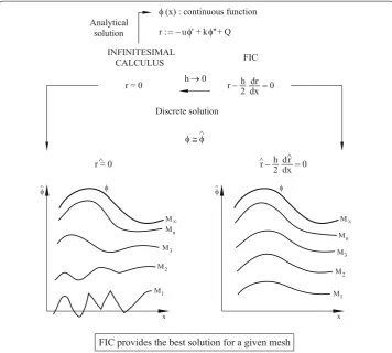
discretization method (i.e. the FE method) leading to the temperature distribution in for specific values of the geometrical and physical parameters. The accuracy of the numerical solution depends on the discretization parameters, such as the number of elements and the particular FE method chosen. Figure2shows a schematic representation of the distributions of ˆφalong a line for different FE discretizationsM1, M2,. . ., Mnwhere
M1andMnare the coarser and finer meshes, respectively. Clearly fornsufficiently large, a good approximation ofφ to the “exact” solution will be obtained. Also, forM∞ the numerical solution ˆφwill coincide with the exact oneφat all points in. Indeed in some problems theM∞ solution can be found at the nodes by a “clever” choice of the FIC parameters in the discretized problem [1,6,10,21,28,32].
The problem arises when for some (typically coarse) discretizations the numerical solu-tion provides non physical or very inaccurate values of ˆφ. The numerical method is then said to beunstable. A situation of this kind is represented by curvesM1andM2of the
left hand side of Fig.2. These unstabilities disappear by an appropriate mesh refinement (curvesM3, M4,. . .) at the obvious increase of the computational cost.
In the FIC formulation the starting point are the modified differential equations of the problem in and the corresponding FIC Neumann boundary condition as previously described. The FIC governing equations can not be used to find an analytical solution, φ(x), for the physical problem. However, the numerical solution of the FIC equations can
be readily found. What is interesting and useful is that, by adequately choosing the values of the characteristic length parameters, the numerical solution of the FIC equations will be always stable for any discretization chosen.
This process is schematically represented in Fig.2where it is shown that the numerical oscillations for the coarser discretizations M1 and M2 disappear when using the FIC
procedure.
In summary the FIC approach allows us to obtain abetter numerical solution for a given discretization. Indeed, as for the standard infinitesimal case, the FIC numerical solution forM∞will yield the (typically unreachable) exact analytical solution and this ensures the consistency of the method.
The FIC method has been classified in [6] as a particular case of “modified equations methods” where the standard differential equations are first augmented using physical concepts and then discretized using a numerical technique. An interpretation of the FIC/FEM equations as a residual correction method is presented in [16].
FIC/FEM solution of advection–diffusion-reaction problems
The FIC form of the advection–diffusion-reaction equation is written (neglecting the FIC term in time) as [21,28]
r− hj 2
∂r ∂xj =
0, r:=ρc
∂φ
∂t +vj∂x∂φ j
−∂x∂
j
k∂φ ∂xj
+sφ−Q, j=1, nd (9)
The new physical parameter in Eq. (9) is the reaction parameters(s>0 is the absorption or dissipation parameter ands<0 is the production parameter).
The boundary conditions at the Dirichlet and Neumann boundary conditions are pre-scribed as explained in a previous section. Recall that the FIC form of the Neumann boundary conditions as defined in Eq. (6) should be used for consistency of the FIC pro-cedure.
Equation (9) solves the following particular problems:
(i) Advection–diffusion (s=0) (ii) Helmholtz (v=0,s<0) (iii) Advection-reaction (k=0) (iv) Diffusion-reaction (v=0)
Finite element discretization
A finite element interpolation of the unknownφcan be written as
φ φˆ = N
i=1
Niφˆi(t) (10)
whereNi(x) are the space shape functions and ˆφiare the nodal values of the approximate function ˆφandNis the number of nodes in the mesh [1–3].
Application of the Galerkin FE method in space to Eqs. (9) and (6) gives, after integrating by parts the term∇∇∇r(and neglecting the space derivatives of the characteristic lengthshj)
Nirdˆ +
q
Ni(nTD∇∇∇φˆ+q¯p)d+ e 1 2 eh T∇∇∇N
iˆrd=0 (11)
I3is the unit matrix),nis the unit vector normal to the boundary,h=[h1, h2, h3]T is the
characteristic length vector andeis the element domain.
The last integral in Eq. (11) has been expressed as a sum of the element contributions to allow for interelement discontinuities in the term∇∇∇rˆ.
Note that the residual terms have disappeared at the Neumann boundary integral in Eq. (11). This is due to taking into account the FIC term in Eq. (6).
Integrating by parts the diffusive terms in the first integral of Eq. (11) gives
Ni
ρc ∂φˆ
∂t +vT∇φˆ
+ ∇∇∇TN
iD∇∇∇φˆ+sφˆ
d+
e 1 2
eh T∇∇∇N
iˆrd
−
NiQd+
q
Niq¯pd =0 (12)
wherev=[v1, v2, v3]Tis the velocity vector. In matrix form
Ca˙+Ka=f with a=[ ˆφ1,φˆ2,· · ·,φˆN]T and a˙:= ∂t∂ a (13) MatricesK,Mand vectorfare assembled from the element contributions given by
Kije=
e[Ni
vT + s
2h T∇∇∇N
j+ ∇∇∇TNi(D+ 1 2hv
T)∇∇∇N j]d
−1 2
eh
T∇∇∇Ni∇∇∇(D∇∇∇N
j)d (14)
Mije =
eρcNi
Nj+ 1 2h
T∇∇∇N j
d;
fie=
e [Ni+
1 2h
T∇∇∇N
i]Qd−
e q
Niq¯pd (15)
The FIC/FEM formulation presented above yields an additional diffusivity matrix and an additional “pseudo” velocity vector given by12hvTands2h, respectively. Also the second integral of Eq. (14) vanishes for linear FEM approximations. The same happens with the second term of the first integral offiin Eq. (15) whenNiis linear andQis constant. The evaluation of these integrals is mandatory in any other case.
This FIC/FEM formulation yields stabilized numerical solutions for the advection– diffusion-reaction equation for a wide range of the physical parameters.
For instance, FIC/FEM solutions for 1D and 2D steady-state advection–diffusion-absorption problems have been respectively obtained by Oñate et al. [21,22] using a non-linear expression for the stabilization parameters. Nodally, exact FIC/FEM solutions for the 1D diffusion–absorption case and the Helmholz equation using a single (linear) sta-bilization parameter were reported by Felippa and Oñate [6] using a variational approach. Oñate, Miquel and Nadukandi [28] have recently presented a general FIC/FEM frame-work for accurately solving the steady-state and transient 1D advection–diffusion-reaction equation using two (linear) stabilization parameters.
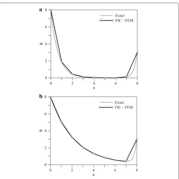
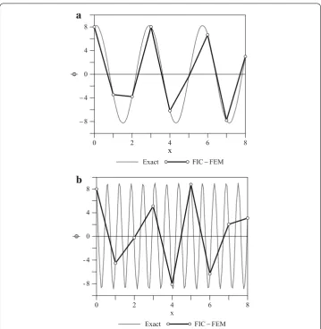
Figure 3 shows FIC/FEM results for two advection–diffusion-absorption problems solved with 2-noded linear elements. Exact nodal values are found [21,28].
Figure4shows the FIC/FEM solution for two Helmholtz problems using 2-noded ele-ments. Again nodally exact results are found [6,28].
A FIC/FEM technique for the transient diffusion equation
a
b
Fig. 3 1D advection–diffusion–absorption problem (Q=0). Exact and FIC–FEM results for a uniform mesh of eight 2-noded elements of lengthle.aγ=1,ω=5;bγ=2,ω=2γ =ρcul2ke,w=s(lke)2[21,28]
et al. [34,35]. This is a general nonincremental iterative non linear solution scheme for time-dependent problems in mechanics which works globally over the entire time-space domain.
Idelsohn et al. [36,37] have proposed a Lagrangian numerical procedure for solving convective-diffusive transport and fluid-flow problems using large time steps.
The FIC approach can also be used for deriving numerical schemes for solving the transient diffusion problem with enhanced features regarding the stability and accuracy of the solution in time. The so-called FIC-time procedure can be summarized as follows. The starting point is the FIC governing equation in time for the standard diffusion problem written as
r+sgδ 2
∂r
∂t =0 with r:=ρc ∂φ ∂t −
∂ ∂xj
k∂φ
∂xj
−Q=0 (16)
whereδis a characteristic time parameter, as mentioned earlier. Typicallyδis chosen as a proportion of the time step chosen for the transient numerical solution.
a
b
Fig. 4 1D Helmholtz problem (Q=0). Exact and FIC–FEM results for a uniform mesh of eight 2-noded elements of lengthle.aγ =0,ω= −5;bγ=0,ω= −100γ =ρcul2ke, w=s(le)2
k
[6,28]
sgδ 2Ca¨+
C+sgδ
2K
˙
a+Ka=f+sgδ
2˙f (17)
Equation (17) is the starting point for deriving a family of new FIC-time integration schemes for the transient diffusion equation. By adequately choosing the characteristic time parameterδand the sign parametersg, the following time integration schemes with improved numerical features can be found [33]:
– Stable explicit solution schemes allowing larger time steps. – Accurate implicit solution schemes allowing larger time steps.
In conclusion, the FIC-time procedure opens a range of possibilities for deriving new improved time integration schemes for solving transient diffusive transport problems with the FEM. The method is also applicable to the FEM solution of Lagrangian flows with larger time steps than using standard time integration schemes.
The FIC approach in fluid mechanics
finite. Following a procedure analogous to that explained in the previous section for the 1D advection–diffusion problem, the momentum balance equation along the ith space direction can be written as
fid= ∂∂
t
ρvid+
(ρvi)v
Tnd i=1, n
d (18)
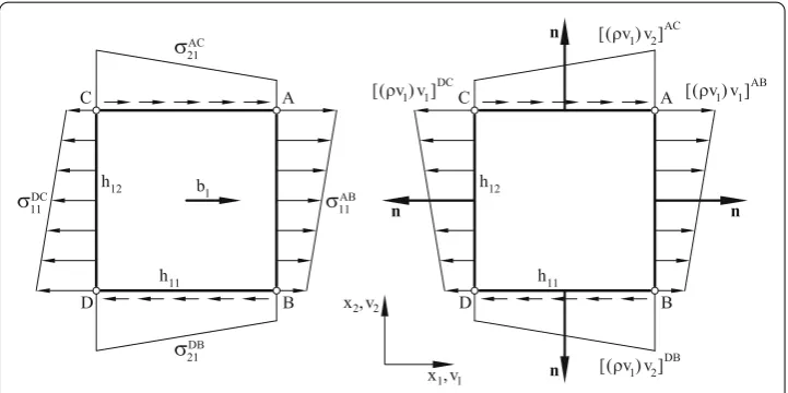
where the different terms in the right-hand-side have been defined earlier andfiincludes the forces due to the stresses acting on the boundaryof the balance domainand the body forcesbi. Figure5shows a typical 2D FIC domain for the balance of momentum along thex1direction. Similar domains are used for the other space directions.
The next step in to express the values of the momentum and force terms at the corner points of the balance domain in terms of those at a reference point within the balance domain using higher order Taylor expansions in the space directions. Retaining second order terms in the expansions, yields the FIC momentum equations in fluid mechanics as [1,12]
¯ rmi−
1 2hij
∂r¯mi ∂xj =
0 i, j=1, nd (19)
wherehijare the sizes of the balance domain (Fig5). For the standard Eulerian formulation in fluid mechanics [2,3]
¯ rmi:=ρ
∂ vi
∂t + ∂ ∂xj
(vivj)
−∂σij
∂xj −
bi (20)
withσij = sij−pδij, wherepis the pressure,δij is the Dirac delta andsijare the viscous deviatoric stresses related to the strain ratesεijand the velocitiesvias
sij=2μ
εij−δij 1 3
∂vk
∂xk
where εij = 1 2
∂v
i
∂xj +
∂vj
∂xi
(21)
Note that distanceh12is arbitrary when writing the balance of momentum along thex1
direction. The same applies for the distanceh21when deriving the balance equation along
thex2direction. Thus, in general,h12=h21.
Mass balance equation
The FIC mass balance equation is obtained by invoking the balance of mass in the finite size domain of Fig.6
ρv
Tnd=0 (22)
Expanding the values ofρviat the corner points in terms of the value at the corner point
Agives the FIC mass balance equation as [1,12]
εv− 1 2hj
∂εv
∂xj =
0 j=1, nd with εv= ∂v∂xi i
(23)
A matrix form of the characteristic distances is not obtained in this case as Eq. (22) expresses the conservation of mass (which is a scalar quantity) in the domain ABCD of Fig.6with dimensionsh1andh2. Distancesh1andh2are in general different from thehij defining the FIC domain where balance of momentum is enforced for each space direction. In practice it is typically assumed thath1=h11andh2=h22for simplicity. The advantage
of choosing thehi distances independently of thehijones can be explored in the search of numerical schemes with enhanced properties for computational fluid mechanics.
Boundary conditions
The FIC Neumann boundary conditions are obtained by expressing the balance of momen-tum in a domain of finite size adjacent to a boundarytwhere the surface tractionstiact. After some algebra we obtain [1,12]
njσij−ti+ 1
2hijnjrmi=0 ont j=1, nd, no sum ini (24a) In Eq. (24a) thehijdistances define the domain where equilibrium of boundary tractions is established. The boundary condition on the Dirichlet boundaryvis the standard one:
vj−vpj =0 on u (24b)
In the discretized problem the characteristic distanceshijandhi become of the order of the typical element dimension. The standard differential equations of momentum and mass balance in fluid mechanics are recovered by making these distances equal to zero.
Eqs. (19), (23) and (24) are the starting point for deriving stabilized FEM for solving the incompressible Navier-Stokes equations. The underlined FIC terms in Eqs. (19) and (24a) suffice for overcoming the numerical instabilities occurring for high Reynolds numbers, whereas the underlined terms in Eq. (23) take care of the eventual instabilities due to the incompressibility constraint.
The discretized system of finite element equations can be obtained by interpolating the velocities and the pressure in terms of nodal values using a mixed FEM formulation and then applying the Galerkin method to the FIC governing equations.
An important feature of the FIC/FEM formulation is that it leads to a stabilized set of equations when using equal order FEM interpolations for the velocity and pressure variables [1,12].
Applications to the FIC/FEM procedure in fluid mechanics
The FIC/FEM procedure has been successfully applied for solving the Navier-Stokes equa-tions for incompressible flow problems using the standard Eulerian formulation presented above [12,19,38,39]. A mixed FEM with a linear interpolation for the velocities and the pressure was used in both cases. FIC/FEM formulations for Stokes flows were reported in [26,40]. Applications of the FIC/FEM technique to fluid-structure interaction (FSI) problems were reported in [14] (for Eulerian flows) and in [41–44] (for Lagrangian flows). The FIC/FEM procedure has been also applied to viscous and inviscid compressible flows as reported in [7–9].
Oñate, Valls and García [23,24] showed that the stabilization terms introduced by the FIC approach in the momentum equation for Eulerian flows provide enough stability for solving high Reynolds number flows with the FEMwithout the need of resorting to a turbulence model. This important feature of the FIC method has been recently extended and exploited by Cotela [4] and Cotela, Oñate and Rossi [5] for the FIC/FEM analysis of a range of incompressible turbulent flow problems.
Figure7presents a 3D simulation of unsteady incompressible flow around a cylinder at a Reynolds number of 10,000. The diameter of the cylinder is 2 units and its length is 8 units. The computation domain extends 15 units upstream, 60 units downstream, and 30 units in the cross flow direction (Fig.7a). The boundary conditions consist of uniform inflow velocity set to 1.0, zero-normal-velocity and zero-shear-stress at the lateral boundaries, traction-free conditions at the outflow boundary and no-slip at the cylinder surface.
The FIC/FEM computation used a structured mesh of some 5 millions linear tetrahedral elements. The thickness of the layer of elements around the cylinder is 0.001. The time step was set to 0.025 s. The time-averaged drag coefficient computed is 1.07 and compares well with the experimental value of 1.12. The Strouhal number computed is 2.02 and also agrees with experimental measurements.
Figures 7c1 show the isosurfaces of the vorticity vector modulus for three different vorticity values. Figure7c2 shows streamlines behind the cylinder within the recirculation area. Details of this problem can be found in [23].
A particle finite element method via FIC
Fig. 7 aComputational domain for 3D flow past a cylinder.bDetails of the mesh used for the computations. (c1) Vorticity vector moduluswisosurfaces:w=0.1,0.2,0.3;w=0.2; (c2) Streamlines at timet=50 [23]
concepts from Lagrangian particle-based techniques and the FEM. In the PFEM the Lagrangian equations of motion for the fluid and solid domains that interact with each other are solved on a finite element mesh which is regenerated at each time step using the information from the nodes that are treated as virtual particles [41]. The physical parameters of the problem are transferred from the nodes to the elements and viceversa at each time step. For the numerical analysis of Lagrangian flows the infinitesimal form of the momentum equations is used. However, the FIC approach is required for stabi-lizing the mass conservationequation in the fluid, which allows using linear elements for interpolating the velocities and the pressure [41].
The good performance of the FIC/PFEM formulation in terms of mass conservation and accuracy for analysis of Lagrangian flows and FSI problems are reported in [44].
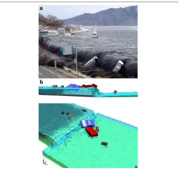
Figures8,9,10and11show examples of application of the PFEM to FSI problems. Figures8and9respectively show the study of the effect of waves impacting on a breakwater and the erosion and failure of a soil mass adjacent to the shore due to the action of the waves. Figure10shows the impact of a landslide on four houses. Finally, Fig.11displays the motion of cars and other objects and debrie particles passing over a vertical wall on a tsunami flow. Other applications of the FIC/PFEM formulation are reported in [38,41–44].
Fig. 9 PFEM analysis of the erosion in a soil mass next to the shore front due to sea waves and the subsequent falling into the sea of a lorry
Fig. 10 PFEM simulation of a landslide falling on four houses
A FIC/FEM formulation for solid mechanics
Application of the FIC method to the equations of equilibrium of forces in solid mechanics leads to the following modified governing equations (for the static case)
ri−
hij 2
∂ri
∂xj =
0 i, j=1, nd with ri:=
∂σij
∂xj +
Fig. 11 Dragging of cars and large and small objects and particles passing over a vertical wall in the Fukushima tsunami (Japan).aThe actual problem.bNumerical results obtained with the PFEM
The deviatoric stress-strain and the strain-displacement relationships have identical form to Eq. (21), respectively substituting the viscosityμby the shear modulusGand the velocitiesviby the displacementsui.
The FIC method can also be applied to derive a modified equation relating the pressure and the volumetric strain change over a finite size domain as [16,18]
1 Kp−εv
−hj
2 ∂ ∂xj
1 Kp−εv
=0, j=1, nd (26)
whereKis the volumetric elastic modulus andεv= ∂∂uxii. For an incompressible material
K → ∞and in this case Eq. (26) recovers a form analogous to that of the stabilized mass balance equation in fluid mechanics (Eq. (23)).
The underlined terms in Eqs. (25) and (26) result from the FIC assumptions and, as usual,hij andhk are the characteristic length parameters. The governing equations are completed with the adequate boundary conditions. Once more, for consistency, the Neu-mann boundary conditions should incorporate a FIC stabilization term as in Eq. (24a) [16,18].
3-noded triangles and 4-3-noded quadrilaterals and tetrahedra with equal order interpolation for the displacements and the pressure [16,18,45].
Error estimation and mesh adaption procedures via FIC
The FIC approach can also be used for deriving a procedure for estimating the error in the numerical solution. The FIC contributions to the discretized form of the modified governing equations can be interpreted as a residual error term that depends on the element size and that tends to zero for very fine meshes and, indeed, it vanishes for the exact solution.
The application of the FIC technique to the estimation of the numerical error can be viewed as a particular class of the so-called residual-based error estimation procedures widely used in computational mechanics [46]. The fact that the residual error estimation terms emerge naturally in the FIC formulation is a distinct feature of the method.
Oñate et al. [20] have used the FIC method for formulating a residual-based error esti-mation technique and the corresponding mesh adaption scheme for analysis of incom-pressible flows with the FEM.
Concluding remarks
The acceptance that the space-time domain where the balance equations are established in mechanics has afinite sizeleads to a modified set of FIC governing differential equations that incorporate the space and time dimensions of the balance domain. The FIC governing equations can be taken as the starting point for deriving a wide range of finite element methods and other numerical techniques with improved features in terms of stability and accuracy for solving steady-state and transient problems of advective–diffusive-reactive transport, fluid dynamics and incompressible solids, among many others.
Acknowledgements
E. Oñate thanks Profs. S.R. Idelsohn, C. Felippa and J. Miquel and Dr. P. Nadukandi for many useful comments. Dedicated to Prof. Pierre Ladevèze on the occasion of his 70th birthday.
Competing interests
The author declares no competing interests.
Received: 19 March 2016 Accepted: 30 March 2016
References
1. Oñate E. Derivation of stabilized equations for numerical solution of advective–diffusive transport and fluid flow problems. Comput Methods Appl Mech Eng. 1998;151(1–2):233–65. doi:10.1016/S0045-7825(97)00119-9. 2. Donea J, Huerta A. Finite element methods for flow problems. Chichester: Wiley; 2003. p. 350. doi:10.1002/
0470013826.http://doi.wiley.com/10.1002/0470013826.
3. Zienkiewicz OC, Taylor RL, Nithiarasu P. The finite element method for fluid dynamics. 6th ed. Oxford: Elsiever Butterworth-Heinemann; 2005.
4. Cotela J. Applications of turbulence modeling in civil engineering. Barcelona: Technical University of Catalonia; 2016. 5. Cotela J, Onate E, Rossi R. A FIC/FEM formulation for analysis of turbulent flows. Research report PI413. Barcelona:
CIMNE; 2016.
6. Felippa CA, Oñate E. Nodally exact Ritz discretizations of 1D diffusion–absorption and Helmholtz equations by variational FIC and modified equation methods. Comput Mech. 2007;39(2):91–111. doi:10.1007/s00466-005-0011-z. 7. Kouhi M, Oñate E. An implicit stabilized finite element method for the compressible Navier-Stokes equations using
finite calculus. Comput Mech. 2015;56(1):113–29. doi:10.1007/s00466-015-1161-2.
8. Kouhi M, Oñate E. A stabilized finite element formulation for high-speed inviscid compressible flows using finite calculus. Int J Numer Methods Fluids. 2014;74(12):872–97. doi:10.1002/fld.3877.
9. Kouhi M, Oñate E, Mavriplis D. Adjoint-based adaptive finite element method for the compressible Euler equations using finite calculus. Aerosp Sci Technol. 2015;46:422–35. doi:10.1016/j.ast.2015.08.008.
11. Oñate E, Manzan M. A general procedure for deriving stabilized space-time finite element methods for advective– diffusive problems. Int J Num Meth Fluids. 1999;31:203–21.
12. Oñate E. A stabilized finite element method for incompressible viscous flows using a finite increment calculus formulation. Comput Methods Appl Mech Eng. 2000;182(3–4):355–70. doi:10.1016/S0045-7825(99)00198-X. 13. Oñate E, Sacco C, Idelsohn S. A finite point method for incompressible flow problems. Comput Vis Sci. 2000;3(1–
2):67–75. doi:10.1007/s007910050053.
14. Oñate E, García J. A finite element method for fluid-structure interaction with surface waves using a finite calculus formulation. Compt Methods Appl Mech Eng. 2001;191(6–7):635–60. doi:10.1016/S0045-7825(01)00306-1. 15. Oñate E. Multiscale computational analysis in mechanics using finite calculus: an introduction. Comput Methods
Appl Mech Eng. 2003;192(28–30):3043–59. doi:10.1016/S0045-7825(03)00340-2.
16. Oñate E, Taylor RL, Zienkiewicz OC, Rojek J. A residual correction method based on finite calculus. Eng Comput. 2003;20(5/6):629–58. doi:10.1108/02644400310488790.
17. Oñate E. Possibilities of finite calculus in computational mechanics. Int J Num Meth Eng. 2004;60(1):255–81. 18. Oñate E, Rojek J, Taylor RL, Zienkiewicz OC. Finite calculus formulation for incompressble solids using linear triangles
and tetrahedra. Int J Numer Methods Eng. 2004;59:1473–500.
19. Oñate E, García J, Idelsohn SR, Pin FD. Finite calculus formulations for finite element analysis of incompressible flows. Eulerian, ALE and Lagrangian approaches. Comput Methods Appl Mech Eng. 2006;195(23–24):3001–37. doi:10.1016/ j.cma.2004.10.016.
20. Oñate E, Arteaga J, García J, Flores R. Error estimation and mesh adaptivity in incompressible viscous flows using a residual power approach. Comput Methods Appl Mech Eng. 2006;195(4–6):339–62. doi:10.1016/j.cma.2004.07.054. 21. Oñate E, Miquel J, Hauke G. Stabilized formulation for the advection–diffusion-absorption equation using finite
calculus and linear finite elements. Comput Methods Appl Mech Eng. 2006;195(33–36):3926–46. doi:10.1016/j.cma. 2005.07.020.
22. Oñate E, Zárate F, Idelsohn SR. Finite element formulation for convective–diffusive problems with sharp gradients using finite calculus. Comput Methods Appl Mech Eng. 2006;195(13–16):1793–825. doi:10.1016/j.cma.2005.05.036. 23. Oñate E, Valls A, García J. Computation of turbulent flows using a finite calculus-finite element formulation. Int J
Numer Methods Fluids. 2007;54(6–8):609–37. doi:10.1002/fld.1476.
24. Oñate E, Valls A, García J. Modeling incompressible flows at low and high Reynolds numbers via a finite calculus-finite element approach. J Comput Phys. 2007;224(1):332–51.
25. Oñate E, Celigueta MA, Idelsohn SR, Salazar F, Suárez B. Possibilities of the particle finite element method for fluid-soil-structure interaction problems. Comput Mech. 2011;48(3):307–18. doi:10.1007/s00466-011-0617-2.
26. Oñate E, Idelsohn SR, Felippa CA. Consistent pressure Laplacian stabilization for incompressible continua via higher-order finite calculus. Int J Numer Methods Eng. 2011;87(1–5):171–95. doi:10.1002/nme.3021.
27. Oñate E, Celigueta MA, Latorre S, Casas G, Rossi R, Rojek J. Lagrangian analysis of multiscale particulate flows with the particle finite element method. Comput Part Mech. 2014;1(1):85–102. doi:10.1007/s40571-014-0012-9.
28. Oñate E, Miquel J, Nadukandi P. An accurate FIC–FEM formulation for the 1D advection–diffusion-reaction equation. Comput Methods Appl Mech Eng. 2016;298:373–406. doi:10.1016/j.cma.2015.09.022.
29. Oñate E, Idelsohn SR, Zienkiewicz OC, Taylor RL. A finite point method in computational mechanics. Applications to convective transport and fluid flow. Int J Numer Methods Eng. 1996;39(22):3839–66.
30. Oñate E, Idelsohn S, Zienkiewicz OC, Taylor RL, Sacco C. A stabilized finite point method for analysis of fluid mechanics problems. Comput Methods Appl Mech Eng. 1996;139(1–4):315–46. doi:10.1016/S0045-7825(96)01088-2. 31. Oñate E, Idelsohn S. A mesh-free finite point method for advective–diffusive transport and fluid flow problems.
Comput Mech. 1998;21(4–5):283–92. doi:10.1007/s004660050304.
32. Oñate E, García J, Idelsohn S. Computation of the stabilization parameter for the finite element solution of advective– diffusive problems. Int J Numer Methods Fluids. 1997;25(12):1385–407.
33. Oñate E, Idelsohn SR, Becker P. A FIC-time approach for deriving enhanced time integration schemes for the transient diffusive equation. Research Report PI414. Barcelona: CIMNE; 2016.
34. Ladevèze P. Nonlinear computational structural mechanics. Mechanical engineering series. New York: Springer; 1999. doi:10.1007/978-1-4612-1432-8.http://link.springer.com/10.1007/978-1-4612-1432-8
35. Ladevèze P, Passieux J-C, Néron D. The LATIN multiscale computational method and the proper generalized decom-position. Comput Methods Appl Mech Eng. 2010;199(21–22):1287–96. doi:10.1016/j.cma.2009.06.023.
36. Idelsohn S, Nigro N, Limache A, Oñate E. Large time-step explicit integration method for solving problems with dominant convection. Compt Methods Appl Mech Eng. 2012;217–220:168–85. doi:10.1016/j.cma.2011.12.008. 37. Idelsohn SR, Marti J, Becker P, Oñate E. Analysis of multifluid flows with large time steps using the particle finite
element method. Int J Numer Methods Fluids. 2014;75(9):621–44. doi:10.1002/fld.3908.
38. Oñate E, Rojek J, Chiumenti M, Idelsohn SR, Pin FD, Aubry R. Advances in stabilized finite element and particle methods for bulk forming processes. Comput Methods Appl Mech Eng. 2006;195:6750–77. doi:10.1016/j.cma.2004.10.018. 39. García J, Oñate E. An unstructured finite element solver for ship hydrodynamics problems. J Appl Mech. 2003;70(1):18.
doi:10.1115/1.1530631.
40. Oñate E, Nadukandi P, Idelsohn SR, García J, Felippa C. A family of residual-based stabilized finite element methods for stokes flows. Int J Numer Methods Fluids. 2011;65(1–3):106–34. doi:10.1002/fld.2468.
41. Oñate E, Idelsohn SR, Del Pin F, Aubry R. The particle finite element method: an overview. Int J Comput Methods. 2004;01(02):267–307. doi:10.1142/S0219876204000204.
42. Oñate E, Idelsohn SR, Celigueta MA, Rossi R. Advances in the particle finite element method for the analysis of fluid-multibody interaction and bed erosion in free surface flows. Comput Meth Appl Mech Eng. 2008;197(19– 20):1777–800. doi:10.1016/j.cma.2007.06.005.
43. Oñate E, Franci A, Carbonell JM. A particle finite element method for analysis of industrial forming processes. Comput Mech. 2014;54(1):85–107. doi:10.1007/s00466-014-1016-2.
45. Rojek J, Oñate E, Taylor RL. CBS-based stabilization in explicit solid dynamics. Int J Numer Methods Eng. 2006;66:1547– 68. doi:10.1002/nme.1689.

![Fig. 7 a Computational domain for 3D flow past a cylinder. b Details of the mesh used for the computations.(c1) Vorticity vector modulus w isosurfaces: w = 0.1, 0.2, 0.3; w = 0.2; (c2) Streamlines at time t = 50 [23]](https://thumb-us.123doks.com/thumbv2/123dok_us/9583189.1941066/13.595.116.478.85.283/computational-cylinder-details-computations-vorticity-modulus-isosurfaces-streamlines.webp)