Full Length Research Article
OPTIMISATION OF PROCESS PARAMETERS FOR WATER-SEA WATER (3%) SYSTEM IN A SPIRAL
PLATE HEAT EXCHANGER (SHE) USING RESPONSE SURFACE METHODOLOGY (RSM)
*Mohamed Shabiulla, A. and Sivaprakasam, S.
Department of Mechanical Engineering, Annamalai University, Tamil Nadu, India
ARTICLE INFO ABSTRACT
In this paper, an attempt is made to optimize the process parameters for Water-Sea Water (3%) system in a Spiral plate Heat Exchanger (SHE). Experiments have been conducted by varying the mass flow rates of cold fluid (Sea Water 3%) and hot fluid (Water) and the inlet temperature of hot fluid by keeping the cold fluid temperature constant. The effects of variables on the process parameters of SHE are studied. The process parameters viz. cold water inlet flow rate (ṁc), hot
water inlet flow rate (ṁh)and hot water inlet temperature (
T
h,in) are optimized using ResponseSurface Methodology (RSM) by solving the regression model equation with Design Expert software and also by analyzing the three-dimensional surface plot in order to maximize the overall heat transfer coefficient (U) and to minimize the pumping power (Wp) in SHE. The most
influential factor on each experimental design response is identified from the analysis of variance (ANOVA). The optimum conditions for SHE proposed by RSM are as follows : i) ṁc - 0.3182
kg/s , ṁh - 0.8470 kg/s and
T
h,in- 60°C. At these optimized conditions, the optimum values of Uand Wp are found to be as follows: U = 1286.985 W/m2 K and Wp = 0.0525 W. A coefficient of
determination (R2) value of 0.9892 for water-sea water (3%) show the fitness of RSM in this work. The optimized values are also verified with experimentation and the results show that the RSM with Box-Behnken design is useful for optimizing the SHE process.
Copyright © 2014 Mohamed Shabiulla, A. and Sivaprakasam, S. This is an open access article distributed under the Creative Commons Attribution License, which permits unrestricted use, distribution, and reproduction in any medium, provided the original work is properly cited.
INTRODUCTION
Heat exchangers are devices which are used to enhance or facilitate the flow of heat. Their application has a wide coverage from industry to commerce. The smallest heat exchanger (<1W) is employed in miniature cryogenic coolers used for infra red thermal imaging. The largest heat exchanger (> I GW) is employed in boilers and condensers. The wide variety of requirements necessiates various types, shapes and flow arrangements in the design and operation of heat exchangers. They are widely used in space heating, refrigeration, air conditioning, power plants, chemical plants, petrochemical plants, petroleum refineries, and natural gas processing. One common example of a heat exchanger is the radiator in a car, in which a hot engine-cooling fluid, like antifreeze, transfers the heat to air flowing through the radiator. Spiral plate heat exchangers are characterized by their large heat transfer surface area per unit volume, resulting in reduced space, weight, support structure, energy requirements
*Corresponding author: Mohamed Shabiulla, A., Department of Mechanical Engineering, Annamalai University, Tamil Nadu, India
and cost, as well as improved process design, plant layout and processing. They have the distinct advantages over other plate type heat exchangers in the aspect that they are self cleaning equipments with low fouling tendencies, easily accessible for inspection and mechanical cleaning. They are best suited to handle slurries and viscous liquids. The use of spiral heat exchangers is not limited to liquid-liquid services. Variations in the basic design of SHEs make them suitable for Liquid-Vapour or Liquid-Gas services. Few literatures have reported about Spiral Heat Exchanger [Holger Martin, 1992; Rangasamy Rajavel and Kaliannagounder Saravanan, 2008; Rajavel and Saravanan, 2008; Manoharan and Saravanan, 2012). Rajavel et al. (2008) have conducted experiments on different process fluids to study the performance of a spiral heat exchanger and developed correlations for different fluid systems. Martin (1992) numerically studied the heat transfer and pressure drop characteristics of spiral plate heat exchanger. Karin Kandananond (2010) used the RSM based Box Behnken design to optimize the various processs parameters in the turning process of AISI 12L14 Steel and ensured that the proposed methodology can be readily applied
ISSN:
2230-9926
International Journal of Development Research
Vol. 4, Issue, 5, pp. 1020-1026, May,2014
International Journal of
DEVELOPMENT RESEARCH
Article History:
Received 13th February, 2014 Received in revised form 01st March, 2014 Accepted 19th April, 2014 Published online 20th May, 2014
Key words:
Spiral plate Heat Exchanger (SHE); Overall Heat Transfer Coefficient (U); Pumping Power (Wp);
in the various turning processes. The effects of cold fluid inlet flow rate (ṁc), hot fluid inlet flow rate (ṁh) and hot fluid inlet
temperature (
T
h,in) on the parameters such as U and WP forfluids like sea water in SHE have not been reported in literature yet. More number of experimental data is required to predict the parameters such as U and WP using mathematical
models like regression analysis. Therefore, an attempt is made in this study to investigate the individual and interactive
effects of ṁc, ṁh and
T
h,in on the parameters such as U andWP for SHE are investigated in this study using Response
Surface Methodology (RSM).
Response surface methodology is a collection of statistical techniques for designing experiments, building models, evaluating the effects of factors and searching for the optimum conditions (Karin Kandananod, 2010; Haghi and Amanifard, 2008). Experiments are designed on the basis of the experimental design technique proposed by Box-Behnken Design(BBD). RSM and BBD are established with the help of the Design Expert software. A quadratic model is used to fit the experimental data obtained in BBD. Analysis of variance (ANOVA) is conducted to test the significance of the fitting model for the experimental data, as well as the significance of the linear terms, interactive terms and the quadratic terms. The parameters are diagnosed by the correlation coefficient, R2, 95% confidence limit, F-value and P-value. In general, the model is considered to be efficient and workable if it has a significant F-value and good R2 (correlation coefficient). Hence, the aim of this study is to determine the relationship
among the factors such as mc,mh and
T
h,in on the Overall HeatTransfer Coefficient (U) and Pumping Power (Wp) for water-
sea water (3% ) system and also to find the optimal conditions in SHE by using RSM.
METHODS
Experimental Set-up and Procedure
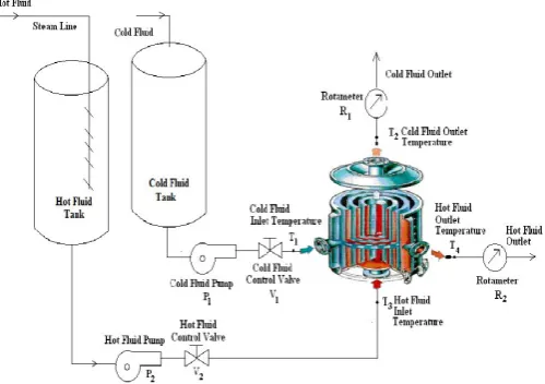
The experimental heat exchanger set-up is shown in Fig.1. The heat exchanger was constructed using 316 stainless steel plates. The end connections are shown in Fig. 1. The dimensions of the spiral plate heat exchanger are tabulated in Table 1. The heat transfer and flow characteristics of water- sea water (3%) system are tested in a spiral plate heat exchanger as shown in Fig. 1. Water is used as the hot fluid. The hot fluid inlet pipe is connected to the central core of the spiral heat exchanger and the outlet pipe is taken from the periphery of the heat exchanger. Hot fluid is heated by pumping steam from the boiler to a temperature of 60°C to 90°C. The hot fluid is pumped to the heat exchanger by using fractional horse power (0.367 kW) pump. Sea water (3%) is used as the cold fluid. The cold fluid inlet pipe is connected to the periphery of the exchanger and the outlet was taken from the centre of the heat exchanger. The cold fluid is supplied at room temperature from a tank and was pumped to the heat exchanger using a fractional horse power (0.367 kW) pump. The inlet hot fluid flow rate and the inlet cold fluid flow rate are varied using the control valves, V1and V2 respectively. Hot
and cold fluid flow paths of heat exchanger are as shown in Figure 1. Thermocouples T4 and T2 are used to measure the
outlet temperature of hot and cold fluids respectively and T3
and T1 are used to measure the inlet temperature of hot and
[image:2.595.312.562.343.519.2]cold fluids respectively. The inlet temperature of the cold fluid is kept constant. For different process conditions viz. hot fluid flow rate, cold fluid flow rate and the inlet temperature, the corresponding outlet temperatures of hot fluid and cold fluid are recorded. Temperature data was recorded in the span of ten seconds. The data used in the calculations are obtained after the system attained steady state. Temperature reading fluctuations are within +/- 0.15°C. Though the type-K thermocouples have limits of error of 2.2°C or 0.75% when placed in a common water solution the readings at steady state are all within +/- 0.1°C. All the thermocouples were constructed from the same roll of thermocouple wire, and hence the repeatability of the temperature readings is high. The operating ranges of different variables are given in Table 2. Experiments are conducted by keeping the cold fluid inlet temperature at 26°C. The experimental data are obtained by varying hot and cold fluid flow rate from 0.1 to 0.9 kg/s for different hot fluid inlet temperatures 60°C, 70°C and 80°C based on the Response Surface Methodology (RSM) using Design Expert software. The experimental results and the corresponding Overall heat transfer coefficient (U) and Pumping Power (Wp) are tabulated in Table 3.
Figure 1. Schematic diagram of the SHE experimental set-up
Table 1. Dimensions of the Spiral Plate Heat Exchanger
Sl.No. Parameter Dimensions
1 Total heat transfer area (m2) 2.24
2 Plate width (mm) 304
3 Plate thickness (mm) 1
4 Plate material 316 Stainless Steel 5 Plate conductivity (W/m° C) 15.364
6 Core diameter (mm) 273
7 Outer diameter (mm) 350
8 Channel spacing (mm) 5
Table 2. experimental conditions
Si.No. Variables Range
1
Hot fluid inlet temperature,
T
h,in 60 - 80 oC 2 [image:2.595.319.549.564.655.2]Process Parameters to be Optimized
Overall heat transfer coefficient (U)
In the case of heat exchangers, various thermal resistances in the path of heat flow from the hot fluid to the cold fluid are combined and represented as the overall heat transfer coefficient (U).The overall heat transfer coefficient is obtained from the relation:
lm Q/(A Δ
U T) (1)
where
U
is the overall heat transfer coefficient (W/m2 K),A
is the heat transfer area (m2) and ΔT is the log mean temperature difference ( K).Pumping power (Wp)
It is the power required to pump the fluid through the flow channel against the pressure drop. Wp is measured in Watt
(W):
fluid the of Density
P) ( drop Pressure x rate flow Volume W
P
(2)
Experimental Design and Data Analysis by RSM
Response Surface Methodology (RSM) has several classes of design, with its own properties and characteristics. Central Composite Design (CCD), Box-Behnken Design and Three Level Factorial Design (TLFD) are the most popular designs applied by the researchers. The Box- Behnken design was used to study the effects of the variables towards their responses and subsequently in the optimization studies. This method is suitable for fitting a quadratic surface and helps to optimize the effective parameters with a minimum number of experiments, as well as to analyse the interaction between the parameters. In order to determine the existence of a relationship between the factors and response variables, the data collected were analysed in a statistical manner using regression. A regression design is normally used in order to model a response as a mathematical function of a few continuous factors. The coded values of the process parameters were determined by the following equation:
i o i i
Δx
X
X
x
(3)where xiis the coded value of the ith variable,Xiis the uncoded value of the ith test variable, X is the uncoded value o of the ith test variable at the center point and Δx iis the step size. The regression analysis was performed to estimate the response function (U and W) as a second-order polynomial
j k
1 i
i k
1 j
ij 2
i k
1 i
ii i
k
1 i
i
0
β
X
β
X
β
X
X
β
Y
(4)
where
Y
is the predicted response, βi ,β
jandβ
ijare coefficients estimated from the regression and they representthe linear, quadratic and cross products of x1,x2andx on 3
response and k is the number of studied factors.
RESULTS AND DISCUSSION
Fitting Models
Experiments are conducted by varying the hot fluid flow rate (ṁh) from 0.1 to 0.9 kg/s, cold fluid flow rate (ṁc) from 0.1 to
0.9 kg/s, inlet temperature of hot fluid (
T
h,in) from 60 to 90oC by keeping the cold fluid inlet temperature at 26oC. The outlet temperatures are recorded for hot fluid and cold fluid. Thevariables ṁh, ṁc and
T
h,inwere chosen as three independentvariables in the experiment design. Fifteen trials are conduced to evaluate the effects of these variables on the overall heat transfer coefficient (U) and pumping power (Wp) which are
[image:3.595.306.560.451.518.2]considered as dependent output variables. Range and levels of independent process variables for water-sea water (3%) system were given in Table 3. The experiment design is given in Table 4 along with experimental data and predicted responses for U and WP. A statistical program package, “Design Expert
7.15” is used for regression analysis of the data obtained and to estimate the coefficient of the regression equation. The equations are validated by the statistical tests called the ANOVA analysis. The significance of each term in the equation is to estimate the goodness of fit in each case. Response surfaces are drawn to determine the individual and interactive effects of test variables, which are first obtained in coded units and are then converted into the uncoded units.
Table 3. Experimental range and levels of independent process variables for water- sea water (3%) system
Fitting models for overall heat transfer coefficient for 3% Sea Water
Experiments are performed according to the Box-Behnken experimental design as given in Table. 4 in order to search for the optimum combination of parameters for obtaining the maxmum overall heat transfer coefficient. A Model F-value of 39.68 implies that the model is significant.There is only a 0.04% chance that the Model F-Value of this large quantity could occur due to noise.The Fisher F test with a probability value as low as 0.0500 demonstrate the significance of the model terms. In this case, A, B, AB, A2, B2 are the significant model terms. The Goodness of Fit of the model is checked by the Coefficient of Determination ( R2 ). In the present case, R2 is calculated as 0.9862. This implies that more than 98 % of the experimental data were compatible with the data predicted by the model and only less than 2% of the total variations are not explained by the model.The R2 value always lies between 0 and 1. A statistical model in which the R2 value very closer to1.0 is considered to be an apt model. Here, in this case, the proposed model can be considered as an apt model.The value of Adjusted R2 (0.9613) is also high to advocate for the high
Codes Independent variable Range and Levels -1 0 +1 A Hot fluid flow rate ( ṁh) kg/s 0.1 0.5 0.9 B Cold fluid flow rate ( ṁc),kg/s 0.1 0.5 0.9 C
[image:3.595.38.290.708.770.2]level of significance of the model. Also, the Predicted R2 value (0.7791) is in reasonable agreement with the Adjusted R2 (0.9613) value. The value of CV % is also low (7.97) which is an indication of the less amount of deviation between the experimental and predicted values. Adequate Precision is a measure of signal to noise ratio. A ratio greater than 4 is desirable. In this work, the ratio is found to be 20.875 which is a clear indication of the adequacy of the model. The experimental results are analyzed using RSM. The results of the theoretically predicted responses are as shown in Table.4. The mathematical expression of relationship to the response with variables is
U = 1166+ 426.25 A+ 251.25 B +0.25 C +161.75 AB -7.25 AC -11.25 BC- 185.12 A2 - 143.13 B2+11.88 C2 (5)
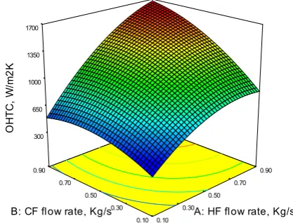
[image:4.595.98.499.87.251.2]where U is the overall heat transfer coefficient and A,B and C are hot fluid flow rate (kg/s ), cold fluid flow rate (kg/s) and hot fluid inlet temperature (oC) respectively. The response surfaces and contour plots are generated for different interaction of any two independent variables, while holding the value of the other variable as constant. Such three dimensional surfaces give accurate geometrical representation and provide useful information about the behaviour of the system within the experimental design. The response surface curves for the overall heat transfer coefficient are shown in Fig.s 2 to 4.
Fig.2 shows the effect of hot fluid and cold fluid flow rates on the overall heat transfer coefficient. From the figure, it is observed that an increase in cold fluid flow rate results in a gradual increase of the overall heat transfer coefficient whereas an increase in the hot fluid flow rate causes a drastic increase in the overall heat transfer coefficient. Hence, the most inflential flow rate among the two is found to be the flow rate of hot fluid.This is because, the hot fluid motion enhances the heat transfer as it brings warmer and cooler chunks of fluid into contact, initiating higher rates of conduction at a greater number of sites. The highest overall heat transfer coefficient, within the design profile, is obtained when the hot and cold water flow rates are maximum. Figs. 3 and 4 show the effect of cold water flow rate alongwith hot water inlet temperature on the overall heat transfer coefficient. From the Figs., it is observed that the increase in hot fluid temperature has minimum influence in increasing the overall heat transfer coefficient. This is because the raise in temperature alone can
[image:4.595.324.533.391.550.2]cause only a slight increase in the overall heat transfer coefficient. The gradual increase of cold fluid flow rate causes a highly significant increase in the overall heat transfer coefficient because of the gradual increase in the fluid motion. A combined effect of increase in both the hot fluid temperature and cold fluid flow rate results in enhancing the overall heat transfer coefficient to the maximum obtainable value. From the plot, it is observed that, among the hot fluid temperature and cold fluid flow rate, the most influential factor is the cold fluid flow rate.
Fig.2. 3D plot showing the effect of cold fluid and hot fluid flow rate on the overall heat transfer coefficient
Fig.3. 3D plot showing the effect of hot water inlet temperature and hot water flow rate on the overall heat transfer coefficient
0.10 0.30
0.50 0.70
0.90
0.10 0.30 0.50 0.70 0.90 300 650 1000 1350 1700
O
H
T
C
,
W
/m
2
K
A: HF flow rate, Kg/s B: CF flow rate, Kg/s
0.10 0.30
0.50 0.70
0.90
60.00 65.00 70.00 75.00 80.00
550 770 990 1210 1430
O
H
T
C
,
W
/m
2
K
A: HF flow rate, Kg/s C: HF inlet temperature, oC
Table 4. BBD matrix for the experimental design and predicted responses for heat transfer coefficient and pumping power using water-sea water (3%) system
Run Coded values Overall Heat transfer Coefficient (U) (W/m
2 K) Pumping power (W p) (W)
A B C Experimental RSM Experimental RSM
1 0 0 0 1165.50 1071.000 0.687 0.770
2 0 0 0 1165.50 1071.000 0.687 0.770
3 0 -1 1 769.80 610.250 0.01 0.017
4 0 -1 -1 737.12 563.250 0.01 0.010
5 1 1 0 1591.89 1590.000 3.82 4.184
6 1 0 1 1461.7 1292.250 0.686 0.736
7 -1 0 -1 509.04 514.750 0.724 0.824
8 0 1 0 1310.02 1227.750 3.84 4.220
9 -1 -1 0 407.10 268.000 0.01 0.006
10 1 0 -1 1485.93 1196.250 0.68 0.774
11 -1 0 1 514.24 538.750 0.718 0.806
12 0 1 -1 1322.19 1154,750 3.89 4.283
13 1 -1 0 826.02 616.500 0.01 0.096
14 -1 1 0 526.21 503.500 3.95 4.394
15 0 0 0 1165.50 1071.000 0.69 0.770
[image:4.595.324.532.593.753.2]Fig.4. 3D plot showing the effect of hot water inlet temperature and hot water inflow rate on the overall heat transfer coefficient
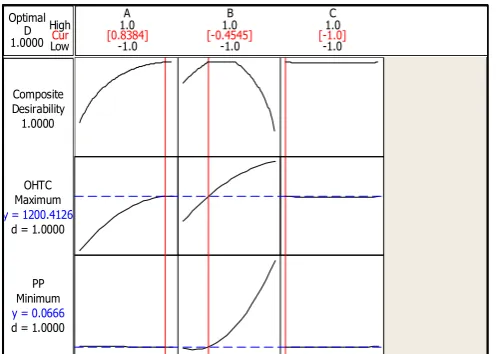
Optimization plot
The optimization chart based on the RSM design is shown below.
The optimum values, to obtain the maximum overall heat transfer coefficient , as inferred from the optimisation plot are,
Hot fluid flow rate = 0.8470 kg/s, Cold fluid flow rate = 0.3182 kg/s. Hot fluid inlet temperature = 60°C.
Under these conditions, the Umax value predicted by the RSM
design is 1200.4126 W/m2K. To verify the accuracy of optimisation by RSM design,experiments are carried out with the above proposed conditions and the experimental value of Umax was found to be 1286.985 W/m2 K. It is observed that the
RSM predicted value of OHTC is 93.27 % accurate to the experimental value.
Fitting models for pumping power for Sea Water (3%)
[image:5.595.316.551.74.190.2]Experiments are performed according to the Box-Behnken experimental design as given in Table. 6 in order to search for the optimim combination of parameters for minimum the pumping power. A Model F-value of 22453.88 implies that the model is significant. There is only a 0.01% chance that the Model F-Value of this large quantity could occur due to noise.The Fisher F test with a probability value as low as 0.0500 demonstrate the significance of the model terms. In this
Table 5. ANOVA for overall heat transfer coefficient
Source Coefficient Factor F Value P Value
Model 2.25E+006 39.68 0.0004
A 1.454E+006 229.99 <0.0001
B 5.05E+005 79.91 0.0003
C 0.5 7.911E-005 0.9932
AB 1.047E+005 16.56 0.0096
AC 210.25 0.033 0.8624
BC 506.25 0.080 0.7885
A2 1.265E+005 20.02 0.0066
B2 75,636.06 11.97 0.0181
C2 520.67 0.082 0.7856
Standard Deviation : 79.50 ; R2 : 0.9862 ; Adjusted R2 : 0.9613 ; Predicted R2 ;
0.7791
Adequate Precision : 20.875 ; C.V.% 7.97.
Table 6. ANOVA for PUMPING POWER
Source Coefficient Factor F Value P Value Model 35.69 22453.88 < 0.0001
A 5.305 E-003 30.04 0.0028
B 29.88 1.692E+005 < 0.0001
C 3.125E-004 1.77 0.2409
AB 4.225E-003 23.92 0.0045
AC 3.600E-005 0.20 0.6705
BC 6.250E-004 3.54 0.1187
A2 5.317E-004 3.01 0.1432
B2 5.75 32537.81 < 0.0001
C2 1.477E-005 0.084 0.7840
Standard Deviation : 0.013 ; R2 : 1.0000 ; Adjusted R2 : 0.9999 ; Predicted R2 :
0.9996;
Adequate Precision ; 363.071 ; C.V.% 0.98.
case, A, B, AB, A2,B2 are the significant model terms. The Goodness of Fit of the model is checked by the Coefficient of Determination ( R2 ). In the present case, R2 is calculated as 1.000. This implies that all of the experimental data were compatible with the data predicted by the model. The R2 value always lies between 0 and 1. A statistical model in which the R2value very closer to1.0 is considered to be an apt model.Here, in this case, the proposed model can be considered as an apt model. The value of Adjusted R2 (0.9999) is also high to advocate for the high level of significance of the model. Also, the Predicted R2 value (0.9996) is also very close to the Adjusted R2 value. The value of CV % is also very low (0.98) which is an indication of the less amount of deviation between the experimental and predicted values. Adequate Precision is a measure of signal to noise ratio.A ratio greater than 4 is desirable. In this work, the ratio is found to be 363.071 which is a clear indication of the adequacy of the model. The experimental results are analyzed using RSM. The results of theoretically predicted responses are as shown in Table.4. The mathematical expression of relationship to the response with variables is
Wp = 0.69-0.026 A+ 1.93 B -6.250E-003 C -0.033AB +3.000
E-003AC -0.012BC+0.012A2 +1.25B2+2.000E-003C2 (6)
where Wp is the pumping power and A,B and C are hot fluid
flowrate (kg/s ), cold fluid flow rate (kg/s) and hot fluid inlet temperature (oC ) respectively.
The response surface and contour plot are generated for different interaction of any two independent variables, while holding the value of the other variables as constant. Such three-dimensional surfaces give accurate geometrical representation and provide useful information about the behaviour of the system within the experimental design. The
0.10 0.30
0.50 0.70
0.90
60.00 65.00 70.00 75.00 80.00
760 895 1030 1165 1300
O
H
TC
,
W
/m
2
K
B: CF flow rate, Kg/s C: HF inlet temperature, oC
Cur
High
Low 1.0000D Optimal
d = 1.0000 Maximum OHTC
y = 1200.4126
d = 1.0000 Minimum
PP
y = 0.0666 1.0000 Desirability Composite
-1.0 1.0
-1.0 1.0
-1.0
[image:5.595.314.554.238.345.2] [image:5.595.40.289.310.487.2]1.0A B C
response surface curves for heat transfer coefficient are shown in Fig.5 to 7. Fig.5 shows the effect of cold fluid and hot fluid flow rates on the pumping power. From the figure, it is observed that an increase in cold fluid flow rate results in a drastic increase of the Wp whereas an increase in the hot fluid
flow rate causes a very slight increase in the Wp. Hence, the
most influential flow rate among the two is found to be the flow rate of the cold fluid. The pumping power consumption is the lowest, within the design profile, when both the cold and hot fluid flow rates are minimum.
Fig.5. 3D plot showing the effect of cold water and hot water flow rate on pumping power
Fig.6. 3D plot showing the effect of hot water inlet temperature and hot water flow rate on pumping power
Fig.7. 3D plot showing the effect of hot water inlet temperature and hot water flow rate on pumping power
The lowest pumping power is noticed when the hot and cold water flow rates are minimum. Figs.6 and 7 show the effect of hot water and cold water flow rates along with hot water inlet temperature on pumping power. From the Fig.6., it is observed that the pumping power consumption decreases as the hot fluid flow rate increases.The hot fluid inlet temperature seems to have no impact on the pumping power.The minimum pumping power conditions are occuring within the design profile. From Fig.7, it is inferred that the hot fluid inlet temperature has almost no impact on the pumping power.Also, the pumping power requirement increases with the increase of cold fluid flow rate. From the pumping power consumption plots, it is confirmed that both the cold and hot fluid flow rates have inflence on the pumping power. Also, among the flow rates, the cold fluid flow rate has comparatively more influence on the pumping power. The optimum values, to run the system with minimum pumping power consumption, as inferred from the optimisation plot are,
Hot fluid flow rate = 0.8470 kg/s , Cold fluid flow rate = 0.3182 kg/s. Hot fluid inlet temperature = 60°C.
Under these conditions, the minimum Wp value predicted by
the RSM design is 0.0666 W.To verify the accuracy of the optimisation by RSM design, a confirmation experiment was carried out with the above proposed conditions and the value of Wp was found to be 0.0525 W. It is observed that the RSM
predicted value of WP is 78.85 % accurate to the experimental
value.
Conclusions
In this study, RSM is used to determine the optimum operating conditions to get the maximum overall heat transfer coefficient while consuming the minimum pumping power in a spiral heat exchnger employing water as the hot fluid and 3% sea water as the cold fluid.Out of the process variables considered for evaluation, the hot fluid flow rate and the cold fluid flow rate are found to be statistically significant.Second order polynomial models were obtained to predict the overall heat transfer coefficient and pumping power.The optimum conditions are found to be : Hot fluid flow rate = 0.8470 kg/s, Cold fluid flow rate = 0.3182 kg/s and Hot fluid inlet temperature = 60 0C. At these optimum conditions, the maximum overall heat transfer coefficient is found to be 1286.985 W/m2 K and is achieved with a minimum pumping power consumption of 0.0525 W.
REFERENCES
Holger Martin, Heat Exchangers, Hemisphere Publishing Corporation, London, 1992.
Rangasamy Rajavel and Kaliannagounder Saravanan, “Heat Transfer Studies on Spiral Plate Heat Exchanger”, Journal of Thermal Science, Vol.12, No.3, pp. 85-90, 2008. Rajavel, R. and K. Saravanan, “An Experimental Study on
Spiral Plate Heat Exchanger for Electrolytes”, Journal of the University of Chemical Technology and Metallurgy, Vol.43, No.2, pp. 255-260, 2008.
Manoharan, K.S. and K. Saravanan, “Experimental Studies in a Spiral Plate Heat Exchanger”, European Journal of Scientific, Vol.75, No.2, pp. 157-162, 2012.
0.10 0.30
0.50 0.70
0.90
0.10 0.30 0.50 0.70 0.90 -0.1 0.925 1.95 2.975 4
P
u
m
p
in
g
p
o
w
e
r,
W
A: HF flow rate, Kg/s B: CF flow rate, Kg/s
0.10 0.30
0.50 0.70
0.90
60.00 65.00 70.00 75.00 80.00 0.672 0.6885 0.705 0.7215 0.738
P
u
m
p
in
g
p
o
w
e
r,
W
A: HF flow rate, Kg/s C: HF inlet temperature, oC
0.10 0.30
0.50 0.70
0.90
60.00 65.00 70.00 75.00 80.00
-0.1 0.9 1.9 2.9 3.9
P
u
m
p
in
g
p
o
w
e
r,
W
Karin Kandananod, “Using the Response Surface Method to Optimize the Turning Process of AISI 12L14 Steel’’, Advances in Mechanical Engineering, Volume 2010, Article ID 392406.
Haghi, A.K. and N.Amanifard, “Analysis of heat and mass transfer during microwave drying of food products’’, Brazilian Journal of Chemical Engineering, Vol.25, No.3, pp.491-501, July-September 2008.