R E S E A R C H
Open Access
Regularized gradient-projection methods for
the constrained convex minimization
problem and the zero points of maximal
monotone operator
Ming Tian
1,2*and Si-Wen Jiao
1*Correspondence:
1College of Science, Civil Aviation
University of China, Tianjin, 300300, China
2Tianjin Key Laboratory for
Advanced Signal Processing, Civil Aviation University of China, Tianjin, 300300, China
Abstract
In this paper, based on the viscosity approximation method and the regularized gradient-projection algorithm, we find a common element of the solution set of a constrained convex minimization problem and the set of zero points of the maximal monotone operator problem. In particular, the set of zero points of the maximal monotone operator problem can be transformed into the equilibrium problem. Under suitable conditions, new strong convergence theorems are obtained, which are useful in nonlinear analysis and optimization. As an application, we apply our algorithm to solving the split feasibility problem and the constrained convex minimization problem in Hilbert spaces.
MSC: 58E35; 47H09; 65J15
Keywords: iterative method; fixed point; constrained convex minimization; maximal monotone operator; resolvent; equilibrium problem; variational inequality
1 Introduction
Throughout this paper, letNandRbe the sets of positive integers and real numbers, respectively. LetHbe a real Hilbert space with the inner product·,·and norm · . Let
Cbe a nonempty, closed, and convex subset ofH. We introduce some operators which will be used in this paper.
A mappingf :C→Cis a contraction if there existsk∈(, ) such thatf(x) –f(y) ≤
kx–yfor allx,y∈C. A nonlinear operatorT:C→Cis called nonexpansive ifTx–
Ty ≤ x–yfor allx,y∈C. The set of fixed points ofTis denoted byFix(T). A nonlinear mappingA:H→His called monotone ifx–y,Ax–Ay ≥ for allx,y∈H.
Firstly, consider the following constrained convex minimization problem:
min
x∈Cg(x), (.)
cursive formula
xn+=PC(I–βn∇g)xn, ∀n≥, (.)
where the parametersβnare real positive numbers, andPCis the metric projection from
H ontoC. It is well known that the convergence of the algorithms (.) depends on the behavior of the gradient ∇g. If the gradient∇g is only assumed to be inverse strongly monotone, then the sequence{xn}defined by the algorithm (.) can only converge weakly
to a minimizer of (.). If the gradient∇gis Lipschitz continuous and strongly monotone, then the sequence generated by (.) can converge strongly to a minimizer of (.) provided the parametersβnsatisfy appropriate conditions.
As we all know, Xu [] gave an averaged mapping approach to the gradient-projection method, and he constructed a counterexample which shows that the sequence generated by the gradient-projection method does not converge strongly in the infinite-dimensional space. Moreover, he presented two modifications of the gradient-projection method which are shown to have strong convergence.
In , motivated by Xu, Cenget al.[] proposed the following iterative algorithm:
xn+=PC
θnγf(xn) + (I–θnμF)Tn(xn)
, n≥, (.)
wheref :C→H is anl-Lipschitzian mapping with a constant l> , andF:C→H is ak-Lipschitzian andη-strongly monotone operator with constantsk,η> . Let <μ< η/k, ≤γl<τ, andτ = – –μ(η–μk). LetT
nandθnsatisfyθn=–λnL,PC(I–
λn∇g) =θnI+ ( –θn)Tn. Under suitable conditions, it is proved that the sequence{xn}∞n=
generated by (.) converges strongly to a minimizerx∗of (.). There are also many other methods for solving constrained convex minimization problems, such as extragradient-projection method (see []) and so on.
However, we all know that the minimization problem (.) has more than one solution under some conditions, so regularization is needed in finding the unique solution of the minimization problem (.). Now, we consider the following regularized minimization problem:
min
x∈Cgα(x) :=g(x) +
α
x
,
whereα> is the regularization parameter,gis a convex function with a /L-ism contin-uous gradient∇g. Then the RGPA generates a sequence{xn}∞n=by the following recursive
formula:
xn+=PC(I–β∇gαn)xn=PC
xn–β(∇g+αnI)(xn)
, (.)
where the parameterαn> ,β is a constant with <β< /L, andPCis the metric
pro-jection fromH ontoC. We all know that the sequence{xn}∞n= generated by algorithm
Secondly, consider the problem of zero points of maximal monotone operator:
B– ={x∈H: ∈Bx}, (.)
where Bis a mapping ofH into H, the effective domain ofBis denoted bydomB or
D(B), that is,domB={x∈H:Bx=∅}. A multi-valued mappingBis said to be a monotone operator onHifx–y,u–v ≥ for allx,y∈domB,u∈Bx,v∈By. A monotone operator
BonHis said to be maximal if its graph is not properly contained in the graph of any other monotone operator onH. For a maximal monotone operatorBonHandr> , we may define a single-valued operatorJr= (I+rB)–:H→domB, which is called the resolvent
ofBforr. We denote byAr=r(I–Jr) the Yosida approximation ofBforr> . We know
from [] that
Arx∈BJrx, ∀x∈H,r> . (.)
LetBbe a maximal monotone operator onH and define the set of zero points ofBas follows:
B– ={x∈H: ∈Bx}.
It is well known thatB– =Fix(Jr) for allr> and the resolventJris firmly nonexpansive,
i.e.,
Jrx–Jry≤ x–y,Jrx–Jry, ∀x,y∈H. (.)
Thirdly, consider the equilibrium problem (EP) which is to findz∈Csuch that
F(z,y)≥, ∀y∈C, (.)
where Fis a bifunction ofC×CintoR, andRis the set of real numbers. We denote the set of solutions of EP byEP(F). Given a mapping T :C→H, letF(x,y) =Tx,y–
x for allx,y∈C, thenz∈EP(F) if and only if Tz,y–z ≥ for ally∈C, i.e., zis a solution of the variational inequality. Numerous problems in physics, optimizations, and economics reduce to finding a solution of (.). Some methods have been proposed to solve the equilibrium problem; see, for instance, [–].
In , Moudafi [] introduced the viscosity approximation method for nonexpansive mappings, extended in []. Letf be a contraction onH, starting with an arbitrary initial
x∈H, define a sequence{xn}recursively by
xn+=αnf(xn) + ( –αn)Txn, n≥, (.)
we useFix(T) to denote the set of fixed points of the mappingT,i.e.,Fix(T) ={x∈H:x=
Tx}.
method in a Hilbert space:x∈Hand
F(un,y) +rny–un,un–xn ≥, ∀y∈C,
xn+=αnf(xn) + ( –αn)T(un), ∀n∈N,
(.)
where{αn} ⊂(, ) and{γn} ⊂(,∞) satisfy some appropriate conditions. Further, they
proved{xn}and{un}converge strongly toz∈Fix(T)∩EP(F), wherez=PFix(T)∩EP(F)f(z).
In , Zenget al.[] proved a strong convergence theorem for finding a common element of the solution set EP of a generalized equilibrium problem and the setT–∩
T– for two maximal monotone operatorsT andTdefined on a Banach spaceX:x∈X
and
xn+=
Hn∩Wn
x, n= , , , . . . ,
where Hn ={z∈ C: φ(z,Krnyn)≤(αn+α˜n–αnα˜n)φ(z,x) + ( –αn)( –α˜n)φ(z,xn)},
Wn={z∈C:xn–z,Jx–Jxn ≥}, x˜n=J–(αnJx+ ( –αn)(βnJxn+ ( –βn)JJrnxn)),
yn=J–(α˜nJx+ ( –α˜n)(β˜nJx˜n+ ( –β˜n)J˜Jrnx˜n)), and{αn},{βn},{ ˜αn},{ ˜βn},{rn}satisfy some appropriate conditions. Then the sequence{xn}converges strongly to
T–∩T–∩EPx,
whereT–∩T–∩EPis the generalized projection ofXontoT–∩T–∩EP.
In , Tian and Liu [] introduced the following iterative method in a Hilbert space:
x∈Cand
F(un,y) +rny–un,un–xn ≥, ∀y∈C,
xn+=αnγf(un) + (I–αnA)Tn(un), ∀n∈N,
(.)
whereF:C×C→R,un=Qβn(xn),PC(I–λn∇g) =θnI+ ( –θn)Tn,θn=–λnL, and{λn} ⊂
(, /L), and{αn},{rn},{θn}, satisfy appropriate conditions. Further, they proved that the
sequence{xn}converges strongly to a pointq∈U∩EP(F), which solves the variational
inequality
(A–γf)q,q–z≤, z∈U∩EP(F).
It is the first time that the equilibrium and constrained convex minimization problems have been solved.
Defining a set-valued mappingAF⊂H×Hby
AFx=
{z∈H:F(x,y)≥ y–x,z,∀y∈C}, ∀x∈C,
∅, ∀x∈/C,
we find from [] thatAFis a maximal monotone operator such that the domain is included
inC; see Lemma . in Section for more details.
In this paper, motivated and inspired by the above results, we introduce a new iterative algorithm:x∈Cand
un=Jrn(xn),
xn+=αnf(xn) + ( –αn)Tλn(un), ∀n∈N
for finding an element ofU∩B–, whereF:C×C→R,T
λn=PC(I–β∇gλn),∇gλn= ∇g+λnI,β∈(, /L). Under appropriate conditions, it is proved that the sequence{xn}
generated by (.) converges strongly to a pointq∈U∩B–, which solves the variational
inequality
(I–f)q,q–z≤, ∀z∈U∩B–.
Equivalently,q=PU∩B–f(q).
Finally, in Section , we apply the above algorithm to the split feasibility problem, and we give concrete examples and the numerical result in Section .
2 Preliminaries
In this section we introduce some properties and lemmas which will be useful in the proofs for the main results in the next section.
Throughout this paper, we always assume thatCis a nonempty closed convex subset of a real Hilbert spaceH. We denote the strong convergence of{xn}tox∈Cbyxn→xand the
weak convergence byxnx. LetFix(T) denote the set of fixed points of the mappingT,
EP(F) denote the solution set of the equilibrium problem (.), andUdenote the solution set of (.). We find that, for anyx,y∈H, the following inequality holds in an inner product spaceX:
x+y≤ x+ y,x+y, ∀x,y∈X. (.)
Firstly, we recall the metric (nearest point) projection fromH ontoCis the mapping
PC:H→Cwhich is defined as follows: givenx∈H,PCxis the unique point inCwith the
property
x–PCx=inf
y∈Cx–y=:d(x,C).
PCis characterized as follows.
Lemma . Given x∈H and y∈C.Then y=PCx if and only if the following inequality
holds:
x–y,y–z ≥, ∀z∈C.
Secondly, we introduce the following lemma, which is about the resolvent of the maxi-mal monotone operator.
Lemma .([, ]; see also []) Let H be a real Hilbert space and let B be a maximal monotone operator on H.For r> and x∈H,define the resolvent Jrx.Then the following
holds:
s–t
s Jsx–Jtx,Jsx–x ≥ Jsx–Jtx
for all s,t> and x∈H.In particular,
Jsx–Jtx ≤
|s–t|/sx–Jsx
Thirdly, for solving the equilibrium problem for a bifunctionF:C×C→R, let us as-sume thatFsatisfies the following conditions:
(A) F(x,x)= for allx∈C;
(A) Fis monotone,i.e.,F(x,y) +F(y,x)≤for allx,y∈C; (A) for eachx,y,z∈C,limt↓F(tz+ ( –t)x,y)≤F(x,y);
(A) for eachx∈C,y→F(x,y)is convex and lower semicontinuous.
Then we have the following lemma, which appears implicitly in Blum and Oettli [].
Lemma .([]) Let F be a bifunction of C×C intoRsatisfying(A)-(A).Let r> and x∈H.Then there exists z∈C such that
F(z,y) +
ry–z,z–x ≥, ∀y∈C.
The following lemma was also given in Combettes and Hirstoaga [].
Lemma .([]) Assume that F:C×C→Rsatisfies(A)-(A).For r> and x∈H,
define a mapping Jr:H→C as follows:
Jr(x) =
z∈C:F(z,y) +
ry–z,z–x ≥,∀y∈C
for all x∈H.Then the following hold:
() Jris single-valued;
() Jris a firmly nonexpansive mapping,i.e.,for allx,y∈H,
Jrx–Jry≤ Jrx–Jry,x–y;
() Fix(Jr) =EP(F);
() EP(F)is closed and convex.
We call suchJrthe resolvent ofFforr> . Using Lemma . and Lemma ., Takahashi
obtained the following lemma. See [] for a more general result.
Lemma .([]) Let H be a Hilbert space and let C be a nonempty,closed,and convex subset of H.Let F:C×C→Rsatisfy(A)-(A).Let AF be a set-valued mapping of H into
itself defined by
AFx=
{z∈H:F(x,y)≥ y–x,z,∀y∈C}, ∀x∈C,
∅, ∀x∈/C.
ThenEP(F) =A–F and AF is a maximal monotone operator withdomAF ⊂C.
Further-more,for any x∈H and r> ,the resolvent Jrof F coincides with the resolvent of AF,i.e.,
Jrx= (I+rAF)–x.
Lemma .([]) Assume that{an}∞n=is a sequence of nonnegative real numbers such that
an+≤( –γn)an+γnδn+βn, n≥,
where{γn}∞n=and{βn}n∞=are sequences in(, )and{δn}∞n=is a sequence inRsuch that (i) ∞n=γn=∞;
(ii) eitherlim supn→∞δn≤or
∞
n=γn|δn|<∞;
(iii) ∞n=βn<∞.
Thenlimn→∞an= .
The so-called demiclosed principle for nonexpansive mappings will often be used.
Lemma .(Demiclosed principle []) Let T:C→C be a nonexpansive mapping with F(T)=∅.If{xn}∞n=is a sequence in C weakly converging to x and if{(I–T)xn}∞n=converges strongly to y,then(I–T)x=y.In particular,if y= ,then x∈F(T).
Lemma .([]) Let C be a nonempty,closed,and convex subset of H and let iCbe the
indicator function of C,then iCis a proper lower semicontinuous convex function on H and
the subdifferential∂iCof iCis a maximal monotone operator.Define Jλx= (I+λ∂iC)–x,for
all x∈H.We see that,for any x∈H and u∈C,u=Jλx⇐⇒u=PCx.
3 Main results
In this section, we will give our main results of this paper. LetBbe a maximal monotone operator onHsuch that the domain ofBis included inC, and define the set of zero points ofBas follows:
B– ={x∈H: ∈Bx}.
We always denoteFix(T) as the fixed point set of the nonexpansive mappingT, denote
U as the solution set of the constrained convex minimization problem (.), and denote
EP(F) as the solution set of the equilibrium problem (.).
Letf be a contraction onCwith the constantk∈(, ). Suppose that ∇g is /L-ism continuous. LetJrn be a sequence of mappings defined as in Lemma .. Consider the mappingGnonCdefined by
Gn(x) =αnf(x) + ( –αn)TλnJrn(x), ∀x∈C,n∈N,
wherePC(I–β∇gλn) =Tλn,∇gλn=∇g+λnI,λn⊂(, /β–L),β∈(, /L),{αn} ⊂(, ). It is easy to prove that∇gλnis
L+λn-ism,Tλnis nonexpansive. It is easy to see thatGnis a contraction. Indeed, by Lemma ., we have, for eachx,y∈C,
Gn(x) –Gn(y)=αnf(x) –αnf(y)
+ ( –αn)
TλnJrn(x) –TλnJrn(y) ≤αnkx–y+ ( –αn)x–y
= –αn( –k)
Since < –αn( –k) < , it follows thatGnis a contraction. Therefore, by the Banach
contraction principle,Gnhas a unique fixed pointxfn∈Csuch that
xfn=αnf
xfn+ ( –αn)TλnJrn
xfn.
For simplicity, we will writexnforxfnprovided no confusion occurs. Then we prove the
convergence of{xn}, while we claim the existence of theq∈U∩B–, which solves the
variational inequality
(I–f)q,p–q≥, ∀p∈U∩B–. (.)
Equivalently,q=PU∩B–f(q).
Theorem . Let H be a real Hilbert space and let C be a nonempty closed convex subset of H.Let B be a maximal monotone operator on H such that the domain of B is included in C.Let Jr= (I+rB)–be the resolvent of B for r> .Let g be a real-valued convex function
of C intoR,and the gradient∇g be a/L-ism with L> .Let f be a contraction with the constant k∈(, ).Assume that U∩B–=∅.Let the sequences{un}and{xn}be generated
by
un=Jrn(xn),
xn=αnf(xn) + ( –αn)Tλn(un), ∀n∈N,
(.)
where Tλn=PC(I–β∇gλn),∇gλn=∇g+λnI,β ∈(, /L).Let{rn},{αn},{λn}satisfy the
following conditions:
(i) {rn} ⊂(,∞),lim infn→∞rn> ;
(ii) {αn} ⊂(, ),limn→∞αn= ;
(iii) {λn} ⊂(, /β–L),λn=o(αn).
Then the sequence{xn}converges strongly to a point q∈U∩B–,which solves the
varia-tional inequality(.).
Proof It is well known thatxˆ∈Csolves the minimization problem (.) if and only if for each fixed <β< /L,xˆsolves the fixed point equation
ˆ
x=PC(I–β∇g)xˆ=Txˆ.
It is clear thatxˆ=Txˆ,i.e.,xˆ∈U=Fix(T).
First, we claim that{xn}is bounded. Indeed, pick anyp∈U∩B–, sinceun=Jrn(xn), andp=Jrn(p), we know that, for anyn∈N,
un–p=Jrn(xn) –Jrn(p)≤ xn–p. (.)
Thus, we derive that
xn–p=αnf(xn) + ( –αn)Tλn(un) –p
+ ( –αn)Tλn(p) –T(p)
≤αnkxn–p+αn(I–f)p+ ( –αn)un–p
+ ( –αn)Tλn(p) –T(p) ≤ –αn( –k)
xn–p+αn(I–f)p+ ( –αn)Tλn(p) –T(p).
It follows that
xn–p ≤
–k(I–f)p+
–αn
αn( –k)
Tλn(p) –T(p). (.)
Forx∈C, note that
PC(I–β∇gλn)x=Tλnx
and
PC(I–β∇g)x=Tx.
Then we get
Tλnx–Tx=PC(I–β∇gλn)x–PC(I–β∇g)x
≤λnβx. (.)
It follows from (.) and (.) that
xn–p ≤
–k(I–f)p+
( –αn)β
–k · λn
αn
p.
Sinceλn=o(αn), there exists a real numberM> such thatλαnn≤M, and
xn–p ≤
–k(I–f)p+
( –αn)β
–k Mp
= (I–f)p+ ( –αn)βMp
–k .
Hence{xn}is bounded and we also find that{un}is bounded.
Next, we show thatxn–un →. Indeed, for anyp∈U∩B–, by Lemma ., we have
un–p=Jrn(xn) –Jrn(p)
≤ xn–p,un–p
=
xn–p+un–p–un–xn
.
This implies that
Then from (.), (.), and (.), we derive that
xn–p=αnf(xn) + ( –αn)Tλn(un) –p
=αnf(xn) –αnp+ ( –αn)
Tλn(un) –p
≤( –αn)Tλn(un) –Tλn(p) +Tλn(p) –T(p)
+ αnf(xn) –p,xn–p
≤( –αn)
un–p+ un–p ·Tλn(p) –T(p)+Tλn(p) –T(p)
+ αnf(xn) –p· xn–p
≤( –αn)
xn–p–un–xn+ un–p ·λnβp+λnβp
+ αn
kxn–p+(I–f)p· xn–p.
Hence, we obtain
( –αn)un–xn≤(αnk–αn)xn–p+ ( –αn)λnβun–p · p
+ ( –αn)λnβp+ αn(I–f)p· xn–p.
Since both{xn}and{un}are bounded andαn→,λn→, it follows thatun–xn →.
Then we show thatxn–Tλn(xn) →. Indeed,
xn–Tλn(xn)=xn–Tλn(un) +Tλn(un) –Tλn(xn)
≤xn–Tλn(un)+Tλn(un) –Tλn(xn)
≤αnf(xn) + ( –αn)Tλn(un) –Tλn(un)+un–xn ≤αnf(xn) –Tλn(un)+un–xn.
Sinceαn→ andun–xn →, we obtainxn–Tλn(xn) →. Thus,
un–Tλn(un)=un–xn+xn–Tλn(xn) +Tλn(xn) –Tλn(un) ≤ un–xn+xn–Tλn(xn)+Tλn(xn) –Tλn(un) ≤ un–xn+xn–Tλn(xn)+xn–un
and
xn–Tλn(un)≤ un–xn+Tλn(un) –un,
we haveun–Tλn(un) → andxn–Tλn(un) →.
Since{un}is bounded, without loss of generality, we can assume thatuniq. Next, we show thatq∈U∩B–.
By (.), we have
un–T(un)≤un–Tλn(un)+Tλn(un) –T(un) ≤un–Tλn(un)+λnβun.
So, by Lemma ., we getq∈Fix(T) =U. Next, we show thatq∈B–. Sinceu
n=Jrn(xn),Bis a maximal monotone operator, we have from (.) Arnixni∈BJrnixni, whereAr is the Yosida approximation ofBforr> . Furthermore, we have, for any (u,v)∈B,
u–uni,v–
xni–uni
rni
≥.
Sincelim infn→∞rn> ,unijqandxnij–unij→, we have
u–q,v ≥.
SinceBis a maximal monotone operator, we have ∈Bqand henceq∈B–. Thus we
haveq∈U∩B–.
On the other hand, we note that
xn–q=αnf(xn) + ( –αn)Tλn(un) –q
=αnf(xn) –αnf(q) +αnf(q) –αnq+ ( –αn)
Tλn(un) –q
.
Hence, we obtain from (.) and (.)
xn–q =αn(f–I)q,xn–q
+ αn
f(xn) –f(q)
+ ( –αn)
Tλn(un) –T(q)
,xn–q
≤αn(f–I)q,xn–q
+αnkxn–q+ ( –αn)Tλn(un) –Tλn(q) +Tλn(q) –T(q)· xn–q
≤αn(f–I)q,xn–q
+αnkxn–q
+ ( –αn)un–q · xn–q+ ( –αn)λnβq · xn–q
≤αn(f–I)q,xn–q
+ ( –αn+αnk)xn–q
+ ( –αn)λnβq · xn–q.
It follows that
xn–q≤
(f –I)q,xn–q
–k +
( –αn)λnβq · xn–q
( –k)αn
.
In particular,
xni–q
≤( –αn)β
–k · λni
αni
q · xni–q+
–k (f–I)q,xni–q
. (.)
Sincexniqandλn=o(αn), it follows from (.) thatxni→qasi→ ∞. Next, we show thatqsolves the variational inequality (.).
Observe that
Hence, we conclude that
(I–f)(xn) = –
αn
(I–TλnJrn)(xn) –TλnJrn(xn) +xn.
SinceTλnJrnis nonexpansive, we find thatI–TλnJrnis monotone. Note that, for any given
z∈U∩B–,
(I–f)(xn),xn–z
= –
αn
(I–TλnJrn)(xn) – (I–TλnJrn)z,xn–z
–
αn
(I–TλnJrn)z,xn–z
– Tλn(un) –xn,xn–z
≤–
αn
(I–TλnJrn)z,xn–z
– Tλn(un) –xn,xn–z
≤
αn
z–Tλn(z)· xn–z+Tλn(un) –xn· xn–z
≤λn
αn
βz · xn–z+Tλn(un) –xn· xn–z.
Now, replacing nwith ni in the above inequality, and lettingi→ ∞, since λn=o(αn),
Tλn(un) –xn →, we have
(I–f)q,q–z=lim
i→∞(I–f)xni,xni–z
≤.
From the arbitrariness ofz∈U∩B–, it follows thatq∈U∩B– is a solution of the
variational inequality (.). Further, by the uniqueness of the solution of the variational inequality (.), we conclude thatxn→qasn→ ∞.
The variational inequality (.) can be rewritten as
f(q) –q,q–z≥, ∀z∈U∩B–.
By Lemma ., it is equivalent to the following fixed point equation:
PU∩B–f(q) =q.
This completes the proof.
Theorem . Let H be a real Hilbert space and let C be a nonempty closed convex subset of H.Let B be a maximal monotone operator on H such that the domain of B is included in C.Let Jr= (I+rB)–be the resolvent of B for r> .Let g be a real-valued convex function
of C intoR,and the gradient∇g be a/L-ism with L> .Let f be a contraction with the constant k∈(, ).Assume that U∩B–=∅.Let the sequences{u
n}and{xn}be generated
by x∈C and
un=Jrn(xn),
xn+=αnf(xn) + ( –αn)Tλn(un), ∀n∈N,
(.)
where Tλn=PC(I–β∇gλn),∇gλn=∇g+λnI,β ∈(, /L).Let{rn},{αn},{λn}satisfy the
(C) {rn} ⊂(,∞),lim infn→∞rn> ,
∞
n=|rn+–rn|<∞;
(C) {αn} ⊂(, ),limn→∞αn= ,
∞
n=αn=∞,
∞
n=|αn+–αn|<∞;
(C) {λn} ⊂(, /β–L),λn=o(αn),
∞
n=|λn+–λn|<∞.
Then the sequence{xn}converges strongly to a point q∈U∩B–,which solves the
varia-tional inequality(.).
Proof It is clear thatxˆ∈Csolves the minimization problem (.) if and only if for each fixed <β< /L,xˆsolves the fixed point equation
ˆ
x=PC(I–β∇g)xˆ=Txˆ,
andxˆ=Txˆ,i.e.,xˆ∈U=Fix(T).
Now, we first show that{xn}is bounded. Indeed, pick anyp∈U∩B–, sinceun=Jrn(xn), by Lemma ., we know that
un–p=Jrn(xn) –Jrn(p)≤ xn–p. (.)
Thus, we derive from (.) that
xn+–p=αnf(xn) + ( –αn)Tλn(un) –p =( –αn)
Tλn(un) –p
+αn
f(xn) –p
≤( –αn)Tλn(un) –Tλn(p) +Tλn(p) –T(p) +αnf(xn) –f(p) +f(p) –p
≤( –αn)
un–p+Tλn(p) –T(p)
+αn
kxn–p+f(p) –p
≤( –αn)
xn–p+λnβp
+αn
kxn–p+f(p) –p
≤ –αn( –k)
xn–p
+αn( –k)
λnβ( –αn)
αn( –k)
p+ αn
αn( –k)
·f(p) –p
.
Sinceλn=o(αn), there exists a real numberE> such thatλαnn≤E. Thus,
xn+–p ≤
–αn( –k)
xn–p+αn( –k)
Eβp+f(p) –p
–k .
By induction, we have
xn–p ≤max
x–p,
–k
Eβp+f(p) –p
, n≥.
Hence,{xn}is bounded. From (.), we also find that{un}is bounded.
Indeed, since∇gis /L-ism,PC(I–β∇gλn) =Tλnis nonexpansive, we derive that
Tλn(un–) –Tλn–(un–)=PC(I–β∇gλn)un––PC(I–β∇gλn–)un–
≤(I–β∇gλn)un–– (I–β∇gλn–)un–
=β∇g(un–) +λn–un––∇g(un–) –λnun–
=β|λn–λn–|un–.
Thus, we get
xn+–xn=αnf(xn) + ( –αn)Tλn(un)
–αn–f(xn–)
+ ( –αn–)Tλn–(un–)
≤αnf(xn) –αnf(xn–)
+αnf(xn–) –αn–f(xn–)
+( –αn)
Tλn(un) –Tλn(un–)
+( –αn)Tλn(un–) – ( –αn)Tλn–(un–)
+( –αn)Tλn–(un–) – ( –αn–)Tλn–(un–)
≤αnkxn–xn–+|αn–αn–| ·f(xn–)
+ ( –αn)un–un–+ ( –αn)Tλn(un–) –Tλn–(un–)
+|αn–αn–| ·Tλn–(un–)
≤αnkxn–xn–+ ( –αn)un–un–
+ ( –αn)β|λn–λn–| · un–
+|αn–αn–|f(xn–)+Tλn–(un–)
≤αnkxn–xn–+ ( –αn)un–un–
+M
|λn–λn–|+|αn–αn–|
(.)
for some appropriate constantM> such that
M≥max
βun–,f(xn–)+Tλn–(un–), ∀n≥.
Sinceun+=Jrn+(xn+) andun=Jrn(xn), we have from Lemma . un+–un=Jrn+xn+–Jrnxn
=Jrn+xn+–Jrn+xn+Jrn+xn–Jrnxn ≤ xn+–xn+|
rn+–rn|
rn+
Jrn+xn–xn.
Sincelim infn→∞rn> , without loss of generality, we may assume that there exists a real
Thus, we have
un+–un ≤ xn+–xn+|
rn+–rn|
a Jrn+xn–xn
≤ xn+–xn+|rn+–rn|M, (.)
whereM=sup{aJrn+xn–xn:n∈N}. From (.) and (.), we obtain
xn+–xn ≤αnkxn–xn–+ ( –αn)un–un–
+M
|λn–λn–|+|αn–αn–|
≤αnkxn–xn–+ ( –αn)
xn–xn–+|rn–rn–|M
+M
|λn–λn–|+|αn–αn–|
≤ –αn( –k)
xn–xn–+M|rn–rn–|
+M
|λn–λn–|+|αn–αn–|
≤ –αn( –k)
xn–xn–
+M
|rn–rn–|+|λn–λn–|+|αn–αn–|
,
whereM=max{M,M}. Hence by Lemma ., we have
lim
n→∞xn+–xn= . (.)
Then, from (.), (.), and|rn+–rn| →, we have
lim
n→∞un+–un= . (.)
For anyp∈U∩B–, in the same way as in the proof of Theorem ., we have
un–p≤ xn–p–un–xn. (.)
Then, from (.) and (.), by the same argument as in the proof of Theorem ., we derive that
xn+–p =( –αn)
Tλn(un) –p
+αn
f(xn) –p
≤Tλn(un) –Tλn(p) +Tλn(p) –T(p)
+ αnTλn(un) –p·f(xn) –p+αnf(xn) –p
≤ xn–p–un–xn+ un–p ·λnβp+λnβp
+αn
un–p+λnβp
·f(xn) –p+f(xn) –p
and hence
xn–un≤ xn–p–xn+–p+ βλnun–p · p+λnβp
+αn
un–p+βλnp
·f(xn) –p+f(xn) –p
≤ xn+–xn
xn–p+xn+–p
+ βλnun–p · p+λnβp
+αn
un–p+βλnp
·f(xn) –p+f(xn) –p
.
Since both{xn},{f(xn)}and{un}are bounded,αn→,λn→, andxn+–xn →, we
have
lim
n→∞xn–un= . (.)
Next, we derive that
xn–Tλn(xn)=xn–xn++xn+–Tλn(un) +Tλn(un) –Tλn(xn)
≤ xn–xn++xn+–Tλn(un)+Tλn(un) –Tλn(xn)
≤ xn–xn++αnf(xn) –Tλn(un)+un–xn.
From (.), (.), andαn→, we have
xn–Tλn(xn)→.
It follows thatun–Tλn(un) →.
Now we show that
lim sup
n→∞
xn–q, –(I–f)q
≤,
whereq∈U∩B– is a unique solution of the variational inequality (.).
Indeed, take a subsequence{xnk}of{xn}such that
lim sup
n→∞
xn–q, –(I–f)q
= lim
k→∞xnk–q, –(I–f)q
. (.)
Since{xn}is bounded, without loss of generality, we may assume thatxnkx˜. By the same argument as in the proof of Theorem ., we havex˜∈U∩B–.
Sinceq=PU∩B–f(q), it follows that
lim sup
n→∞
(I–f)q,q–xn
= (I–f)q,q–x˜≤. (.)
Finally, we show thatxn→q.
In fact,
xn+–q=αnf(xn) + ( –αn)Tλn(un) –q =αn
f(xn) –f(q)
+αn
f(q) –q
+ ( –αn)
Tλn(un) –Tλn(q)
+ ( –αn)
Tλn(q) –T(q)
So, from (.) and (.), we derive
xn+–q= ( –αn) Tλn(un) –Tλn(q)
+Tλn(q) –T(q)
,xn+–q
+αnf(xn) –f(q),xn+–q
+αn–(I–f)q,xn+–q
≤( –αn)
un–q+λnβq
xn+–q
+αnkxn–q · xn+–q+αn–(I–f)q,xn+–q
≤( –αn)xn–q · xn+–q+ ( –αn)λnβq · xn+–q
+αnkxn–q · xn+–q+αn–(I–f)q,xn+–q
≤ –αn( –k)
xn–q · xn+–q+λnβq · xn+–q
+αn–(I–f)q,xn+–q
≤ –αn( –k)
xn–q+xn+–q
+αn –(I–f)q,xn+–q
+λn
αn
βq · xn+–q
.
It follows that
xn+–q≤
–αn( –k)
+αn( –k)
xn–q
+ αn
+αn( –k)
–(I–f)q,xn+–q
+λn
αn
βq · xn+–q
≤ –αn( –k)
xn–q
+ αn
+αn( –k)
–(I–f)q,xn+–q
+λn
αn
βq · xn+–q
;
since{xn}is bounded, we can take a constantM> such that
M≥ xn+–q, n≥.
Then we obtain
xn+–q≤
–αn( –k)
xn–q+αnδn, (.)
whereδn=+αn(–k)[–(I–f)q,xn+–q+
λn
αnβqM].
By (.) andλn=o(αn), we getlim supn→∞δn≤. Now applying Lemma . to (.)
one concludes thatxn→qasn→ ∞. The variational inequality (.) can be rewritten as
f(q) –q,q–z≥, ∀z∈U∩B–.
By Lemma ., it is equivalent to the following fixed point equation:
PU∩B–f(q) =q.
4 Applications
In this section, we will give some applications, which are useful in nonlinear analysis and optimization.
Theorem . Let H be a real Hilbert space and let C be a nonempty closed convex subset of H.Let F be a bifunction of C×C intoRsatisfying(A)-(A).Let Jrbe the resolvent of F for
r> .Let g be a real-valued convex function of C intoR,and the gradient∇g be a/L-ism with L> .Let f be a contraction with the constant k∈(, ).Assume that U∩EP(F)=∅.
Let the sequences{un}and{xn}be generated by x∈C and
F(un,y) +rny–un,un–xn ≥, ∀y∈C,
xn+=αnf(xn) + ( –αn)Tλn(un), ∀n∈N,
(.)
where Tλn=PC(I–β∇gλn),∇gλn=∇g+λnI,β ∈(, /L).Let{rn},{αn},{λn}satisfy the
conditions(C)-(C).Then the sequence{xn}converges strongly to a point q∈U∩EP(F),
where q=PU∩EP(F)f(q).
Proof For a bifunctionFofC×CintoRsatisfying (A)-(A), we can define a maximal monotone operatorAFwithdomAF⊂C. PutB=AFin Theorem .. Then by Lemma .,
we haveun=Jrn(xn). Thus we obtain the desired result by Theorem ..
On the other hand, based on Theorem . and Theorem ., we will give another two applications of it. In , Censor and Elfving [] introduced the split feasibility problem (SFP). Then various algorithms were introduced by some authors to solve it (see [] and [–]). Recently, many authors have paid attention to the SFP due to its application in signal processing and image reconstructions (see [, , ]).
LetCandQbe nonempty, closed, and convex subset of real Hilbert spacesHandH,
respectively. Then the SFP under consideration in this paper can mathematically be for-mulated as finding a pointxsatisfying the following property:
x∈C and Ax∈Q, (.)
whereA:H→His a bounded linear operator. It is clear thatx∗is a solution to the split
feasibility problem (.) if and only ifx∗∈CandAx∗–PQAx∗= . We define the proximity
functiongby
g(x) =
Ax–PQAx
.
Then consider the constrained convex minimization problem
min
x∈Cg(x) =minx∈C
Ax–PQAx
. (.)
Thenx∗solves the SFP (.) if and only ifx∗solves the minimization problem (.) with the minimum equal to .
In particular, the so-calledCQalgorithm was introduced by Byrne []. Take the initial guessx∈Harbitrarily, and define{xn}recursively as follows:
xn+=PC
I–βA∗(I–PQ)A
where <β< /AandP
Cdenotes the projector ontoC. Then the sequence{xn}
gen-erated by (.) converges weakly to a solution of the SFP.
LetBbe a maximal monotone operator on Hilbert spaceH. LetJr= (I+rB)–be the
resolvent ofBforr> . In order to obtain a strong convergence iterative sequence to solve the SFP, we propose a new algorithm as follows:x∈C,
un=Jrn(xn),
xn+=αnf(xn) + ( –αn)Tλn(un), ∀n∈N,
(.)
where f :C→C is a contraction with the constantk∈(, ), and{Tλn}satisfy PC(I–
β(A∗(I–PQ)A+λnI)) =Tλnfor alln, andβ∈(, /A). We can show that the sequence {xn}generated by (.) converges strongly to a solution of the SFP (.) if the sequence
{αn} ⊂(, ) and the sequence{λn}of parameters satisfy appropriate conditions. Applying
Theorem ., we obtain the following result.
Theorem . Assume that the split feasibility problem(.)is consistent.Let the sequence
{xn}be generated by(.).Here the sequences{rn}and{αn} ⊂(, ),and the sequence{λn}
satisfy the conditions(C)-(C).Then the sequence{xn}converges strongly to a point q∈
W∩B–,where W denotes the solution set of SFP(.).
Proof By the definition of the proximity functiong, we have
∇g(x) =A∗(I–PQ)Ax,
sincePQis /-averaged mapping, thenI–PQis -ism, for∀x,y∈C, we obtain
∇g(x) –∇g(y),x–y– /A·∇g(x) –∇g(y)
= A∗(I–PQ)Ax–A∗(I–PQ)Ay,x–y
– /A·A∗(I–PQ)Ax–A∗(I–PQ)Ay
= A∗(I–PQ)Ax– (I–PQ)Ay
,x–y
– /A·A∗(I–PQ)Ax– (I–PQ)Ay
= (I–PQ)Ax– (I–PQ)Ay,Ax–Ay
– /A·A∗(I–PQ)Ax– (I–PQ)Ay
≥(I–PQ)Ax– (I–PQ)Ay
–(I–PQ)Ax– (I–PQ)Ay
= .
So,∇gis /A-ism.
Setgλn(x) =g(x) +λnx, consequently,
∇gλn(x) =∇g(x) +λnI(x)
Then the iterative scheme (.) is equivalent to
un=Jrn(xn),
xn+=αnf(xn) + ( –αn)Tλn(un), ∀n∈N,
where{Tλn}satisfyPC(I–β(A∗(I–PQ)A+λnI)) =Tλnfor alln, andβ∈(, /A
).
However, in order to obtain a strong convergence iterative sequence to solve the SFP, we propose another new algorithm as follows:x∈C,
F(un,y) +rny–un,un–xn ≥, ∀y∈C,
xn+=αnf(xn) + ( –αn)Tλn(un), ∀n∈N,
(.)
where f :C→C is a contraction with the constantk∈(, ), and{Tλn}satisfy PC(I–
β(A∗(I–PQ)A+λnI)) =Tλnfor alln, andβ∈(, /A). We can show that the sequence {xn}generated by (.) converges strongly to a solution of the SFP (.) if the sequence
{αn} ⊂(, ) and the sequence{λn}of parameters satisfy appropriate conditions. Applying
Theorem ., we obtain the following result.
Theorem . Assume that the split feasibility problem(.)is consistent.Let the sequence
{xn} be generated by(.).Here the sequences {rn}and{αn} ⊂(, ),the sequence {λn}
satisfies the conditions (C)-(C). Then the sequence {xn} converges strongly to a point
q∈W∩EP(F),where W denotes the solution set of SFP(.).
Proof For a bifunctionFofC×CintoRsatisfying (A)-(A), we can define a maximal monotone operatorAFwithdomAF⊂C. PutF=AFin Theorem .. Then by Lemma .,
we haveun=Jrn(xn). Thus we obtain the desired result by Theorem . and Theorem ..
5 Numerical results
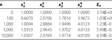
In this section, we present the following concrete examples to judge the numerical per-formance of our algorithm. By using the algorithm in Theorem . and Theorem ., we illustrate its realization, effectiveness, and convergence in solving a system of linear equa-tions and a constrained convex minimization problem.
The first example is the × system of linear equations, which use the algorithm in Theorem ..
Example In Theorem ., we assume thatH=H=R. Takef =I, whereIdenotes
the × identity matrix. Given the parametersαn= n+, λn= (n+) for every n≥.
β= . Take
A=
⎛ ⎜ ⎜ ⎜ ⎝
– –
– –
–
⎞ ⎟ ⎟ ⎟
⎠, (.)
b=
⎛ ⎜ ⎜ ⎜ ⎝
– –
⎞ ⎟ ⎟ ⎟
Table 1 Numerical results as regards Example 1
n x1
n x2n xn3 xn4 En
0 1.0000 1.0000 1.0000 1.0000 3.74E+00 100 0.6070 2.0706 1.7816 3.9672 1.03E+00 1,000 1.0094 2.8884 1.9496 4.0123 1.23E–01 5,000 1.0353 2.9643 1.9702 4.0133 5.99E–02 10,000 1.0307 2.9769 1.9774 4.0109 4.59E–02
The SFP can be formulated as the problem of finding a pointx∗with the property
x∗∈C and Ax∗∈Q,
whereC=H,Q={b} ⊂H. That is,x∗is the solution of the system of linear equations Ax=b, and
x∗=
⎛ ⎜ ⎜ ⎜ ⎝ ⎞ ⎟ ⎟ ⎟ ⎠. (.)
Then by Theorem . and Lemma ., the sequence{xn}is generated by
xn+=
(n+ )xn+
n+
n+
xn–
A ∗Ax n+ A
∗b– (n+ )xn
.
Asn→ ∞, we have{xn} →x∗= (, , , )T.
From Table , we can easily see that with iterative number increasing,xnapproaches the
exact solutionx∗and the errors gradually approach zero.
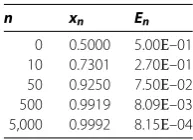
The second example is also the constrained convex minimization problem, which uses the algorithm in Theorem ..
Example In Theorem ., we assume thatH=RandC= [, ]. Take f =I, where
I denotes the unit function. Given the parametersαn=n+,λn=(n+) for everyn≥.
β=. Consider the problem (.) and take the function
g(x) =–x
ex, ∀x∈C. (.)
The problem (.) can be written as
min
x∈[,]
–x
ex. (.)
It is easy to see that∇gis /-ism, that is,L= . In order to solve the problem (.), we can find a pointx∗∈[, ], such thatg(x) reaches the minimum atx∗, andx∗= .
Then by Theorem . and Lemma ., the sequence{xn}is generated by
xn+=
(n+ )xn+
n+
n+ PC
xn–
xn
exn –
exn + (n+ )xn
.
Table 2 Numerical results as regards Example 2
n xn En
0 0.5000 5.00E–01 10 0.7301 2.70E–01 50 0.9250 7.50E–02 500 0.9919 8.09E–03 5,000 0.9992 8.15E–04
From Table , we easily see that by using the regularization method and with iterative number increasing,xnapproaches tox∗and the errors gradually approach to zero.
From the computer programming’s point of view, the above algorithms in the concrete examples are easier to implement in this paper.
6 Conclusion
In a real Hilbert space, methods for solving the equilibrium problem and constrained con-vex minimization problem have been extensively studied, respectively. Recently, Tian and Liu were first to propose composite iterative algorithms for finding a common solution of an equilibrium and a constrained convex minimization problem. However, in this paper, we use the regularized gradient-projection algorithm to find the unique solution of the problems of constrained convex minimization problem and the zero points of maximal monotone operator, which also solves a certain variational inequality. In particular, un-der suitable conditions, the zero points of a maximal monotone operator problem can be transformed into the equilibrium problem. Then new strong convergence theorems and applications are obtained, which also solve a certain variational inequality. Finally, we ap-ply this algorithm to the split feasibility problem and the constrained convex minimization problem, and we illustrate the effectiveness, realization, and convergence of our algorithm by giving concrete examples and numerical results.
Competing interests
The author declare that they have no competing interests.
Authors’ contributions
All the authors read and approved the final manuscript.
Acknowledgements
The authors thank the referees for their helping comments, which notably improved the presentation of this paper. This work was supported by the Foundation of Tianjin Key Laboratory for Advanced Signal Processing.
Received: 19 September 2014 Accepted: 2 January 2015 References
1. Xu, HK: Averaged mappings and the gradient-projection algorithm. J. Optim. Theory Appl.150, 360-378 (2011) 2. Ceng, LC, Ansari, QH, Yao, JC: Some iterative methods for finding fixed points and for solving constrained convex
minimization problems. Nonlinear Anal.74, 5286-5302 (2011)
3. Ceng, LC, Ansari, QH, Yao, JC: Extragradient-projection method for solving constrained convex minimization problems. Numer. Algebra Control Optim.1(3), 341-359 (2011)
4. Xu, HK: Iterative methods for the split feasibility problem in infinite-dimensional Hilbert spaces. Inverse Probl.26, 105018 (2010)
5. Ceng, LC, Ansari, QH, Wen, CF: Multi-step implicit iterative methods with regularization for minimization problems and fixed point problems. J. Inequal. Appl.2013, Article ID 240 (2013)
6. Takahashi, W: Convex Analysis and Approximation of Fixed Points. Yokohama Publishers, Yokohama (2000) 7. Flam, SD, Antipin, AS: Equilibrium programming using proximal-like algorithms. Math. Program.78, 29-41 (1997) 8. Takahashi, S, Takahashi, W: Viscosity approximation methods for equilibrium problems and fixed point problems in
Hilbert spaces. J. Math. Anal. Appl.331, 506-515 (2007)
10. Qin, XL, Cho, YJ, Kang, SM: Convergence analysis on hybrid projection algorithms for equilibrium problems and variational inequality problems. Math. Model. Anal.14, 335-351 (2009)
11. Combettes, PL, Hirstoaga, SA: Equilibrium programming in Hilbert spaces. J. Nonlinear Convex Anal.6, 117-136 (2005) 12. Moudafi, A: Viscosity approximation method for fixed-points problems. J. Math. Anal. Appl.241, 46-55 (2000) 13. Marino, G, Xu, HK: A general method for nonexpansive mappings in Hilbert space. J. Math. Anal. Appl.318, 43-52
(2006)
14. Zeng, LC, Ansari, QH, Shyu, DS, Yao, JC: Strong and weak convergence theorems for common solutions of generalized equilibrium problems and zeros of maximal monotone operators. Fixed Point Theory Appl.2010, Article ID 590278 (2010)
15. Tian, M, Liu, L: General iterative methods for equilibrium and constrained convex minimization problem. Optimization63(9), 1367-1385 (2014)
16. Takahashi, S, Takahashi, W, Toyoda, M: Strong convergence theorems for maximal monotone operators with nonlinear mappings in Hilbert spaces. J. Optim. Theory Appl.147, 27-41 (2010)
17. Eshita, K, Takahashi, W: Approximating zero points of accretive operators in general Banach spaces. JP J. Fixed Point Theory Appl.2, 105-116 (2007)
18. Takahashi, W: Nonlinear Functional Analysis. Yokohama Publishers, Yokohama (2000)
19. Blum, E, Oettli, W: From optimization and variational inequalities to a equilibrium problems. Math. Stud.63, 123-145 (1994)
20. Aoyama, K, Kimura, Y, Takahashi, W: Maximal monotone operators and maximal monotone functions for equilibrium problems. J. Convex Anal.15, 395-409 (2008)
21. Hundal, H: An alternating projection that does not converge in norm. Nonlinear Anal.57, 35-61 (2004)
22. Lin, LJ, Takahashi, W: A general iterative method for hierarchical variational inequality problems in Hilbert spaces and applications. Positivity16, 429-453 (2012)
23. Censor, Y, Elfving, T: A multiprojection algorithm using Bregman projections in a product space. Numer. Algorithms8, 221-239 (1994)
24. Byrne, C: A unified treatment of some iterative algorithms in signal processing and image reconstruction. Inverse Probl.20, 103-120 (2004)
25. Byrne, C: Iterative oblique projection onto convex sets and the split feasibility problem. Inverse Probl.18(2), 441-453 (2002)
26. Qu, B, Xiu, N: A note on the CQ algorithm for the split feasibility problem. Inverse Probl.21(5), 1655-1662 (2005) 27. Xu, HK: A variable Krasnosel’skii-Mann algorithm and the multiple-set split feasibility problem. Inverse Probl.22(6),
2021-2034 (2006)
28. Yang, Q: The relaxed CQ algorithm solving the split feasibility problem. Inverse Probl.20(4), 1261-1266 (2004) 29. Yang, Q, Zhao, J: Generalized KM theorems and their applications. Inverse Probl.22(3), 833-844 (2006) 30. Lopez, G, Martin-Marquez, V, Wang, FH, Xu, HK: Solving the split feasibility problem without prior knowledge of
matrix norms. Inverse Probl.28, 085004 (2012)