R E S E A R C H
Open Access
Iterative methods for solving the
multiple-sets split feasibility problem with
splitting self-adaptive step size
Yuchao Tang
1*, Chuanxi Zhu
1and Hui Yu
2*Correspondence:
1Department of Mathematics,
Nanchang University, Nanchang, 330031, P.R. China
Full list of author information is available at the end of the article
Abstract
We introduce an iterative algorithm for solving the multiple-sets split feasibility problem with splitting self-adaptive step size. This step size is calculated directly from the iteration process without need to know the spectral norm of linear operators. We also generalize the chosen step size to a relaxed iterative algorithm. Theoretical convergence is proved in an infinite dimensional Hilbert space. Some numerical experiments are presented to verify the effectiveness of our proposed methods.
MSC: 90C25; 90C30; 47J25
Keywords: multiple-sets split feasibility problem; self-adaptive step size; compressive sensing; lasso problem
1 Introduction
Linear inverse problems often arise in many real-world application problems such as sig-nal and image processing, medical image reconstruction,etc.In , Censoret al.[] first introduced the multiple-sets split feasibility problem, which was motivated by the in-verse problem of intensity modulated radiation therapy (IMRT). The multiple-sets split feasibility problem (MSSFP for short) required to find a point closest to the intersection of a family of closed convex sets in one space such that its image under a linear transfor-mationAwill be closest to the intersection of another family of closed convex sets in the image space. The MSSFP includes the two-set split feasibility problem as its special case, which was originally proposed by Censor and Elfving []. The two-set split feasibility prob-lem is usually called the split feasibility probprob-lem (SFP) for simple. Byrne [, ] proposed the so-called CQ algorithm to solve the SFP. It has been proved that the CQ algorithm is equivalent to the gradient projection algorithms for solving a constrained optimization problem, see, for example, Xu [].
The CQ algorithm used a fixed step size, which relies on the spectral norm of the linear operatorA. Qu and Xiu [] improved it by using the Armijo-like search method to solve the SFP, for which there is no need to know the prior norm ofA. They also used the Armijo-like search way to a relaxed CQ algorithm. The relaxed CQ algorithm with constant step size was introduced by Yang []. It was used to solve the SFP, where the closed convex sets are level sets of convex functions. In comparison with the CQ algorithm, the relaxed
CQ algorithm used orthogonal projections onto half-spaces instead of projections onto the original convex sets. Since projections onto half-spaces can be directly calculated, it reduced a lot of work for computing projections. Lopezet al.[] introduced a new self-adaptive step size to improve the CQ and the relaxed CQ algorithm, which also did not require to know the norm ofA. This step size is a modification of Yang []. They proved the convergence of an iterative sequence with the new self-adaptive step size and weakened the assumptions used by Yang [].
Since the intersection of a family of closed convex sets is also a closed convex set, the MSSFP could be viewed as the SFP as well. However, the iterative projection methods for solving the SFP cannot be directly transferred to solve the MSSFP because one needs to calculate the projection of the intersection of a family of sets instead of a single set. To solve the MSSFP, Censoret al.[] defined a function (see ()) to measure the distance of a point to all sets and proposed a gradient projection algorithm. In [], Xu transferred the MSSFP to finding a common fixed point of a finite family of averaged mappings. Then, he proposed several iterative algorithms to solve the MSSFP, which was inspired by fixed point searching methods. Note that these iterative algorithms also used a fixed step size. To overcome this shortage, Zhanget al.[] proposed a self-adaptive projection method for solving the MSSFP, which was inspired by the work of Heet al.[]. Zhao and Yang [] generalized the method used in [] to solve the MSSFP and also gave a self-adaptive projection method. These iterative algorithms have a common feature that an inner iter-ation number should be chosen before the updated iterative sequence. See also [–]. Recently, Zhao and Yang [] introduced a simple self-adaptive step size way to solve the MSSFP. The new step size is computed by the objective function and its gradient informa-tion without an inner iterainforma-tion number. Inspired by this idea, Wenet al.[] also suggested a self-adaptive step size to improve the results of Xu []. They proposed a cyclic and si-multaneous iterative sequence with self-adaptive step size to solve the MSSFP.
In this paper, we propose a new iterative algorithm for solving the multiple-sets split feasibility problem. The new iterative algorithm is combined with a splitting self-adaptive step size. Thus, we need not know the prior norm of the linear operator. Further, we give a relaxed version of this iterative algorithm to solve the MSSFP where the closed convex sets are level sets of convex functions. The theoretical convergence results are proved in infinite dimensional Hilbert spaces. To verify the effectiveness of our proposed methods, we also give some numerical experiments.
The paper is organized as follows. In the next section, we introduce some definitions and lemmas, which will be used in the following. In Section , we propose an iterative al-gorithm with splitting self-adaptive step size and prove its convergence. Further, a relaxed iterative algorithm with splitting self-adaptive step size will be proposed in Section . In Section , we present some preliminary numerical experiments to test these proposed methods and compare with other methods. We give some conclusions in the final section.
2 Preliminaries
LetHbe a real Hilbert space,·,·and·be the inner product and the norm, respectively, inH. We adopt the following notations:denotes the solution set of the MSSFP;xk→x
(xkx) represents{xk}converging strongly (weakly) tox, respectively;ω
w(xk) means the
weak cluster of the sequence{xk}.
Definition .([]) LetT be a mapping fromC⊆HintoH. Then (i) Tis said to be nonexpansive ifTx–Ty ≤ x–y,∀x,y∈C;
(ii) Tis said to be firmly nonexpansive ifx–y,Tx–Ty ≥ Tx–Ty,∀x,y∈C;
(iii) Tis said to be an averaged mapping if there exist a nonexpansive mappingSand a real numbert∈(, )satisfyingT= ( –t)I+tS, whereIrepresents the identity mapping.
It is easily seen that a firmly nonexpansive mapping is nonexpansive due to the Cauchy-Schwarz inequality. Recall that the orthogonal projectionPC fromH onto a nonempty
closed convex subsetC⊂His defined by the following:
PC(x) =arg min y∈Cx–y.
The orthogonal projection has the following well-known properties.
Lemma .([]) Let C be a nonempty closed and convex set in H,then for all x,y∈H and z∈C,
(i) x–PCx,z–PCx ≤;
(ii) PCx–PCy≤ PCx–PCy,x–y;
(iii) PCx–z≤ x–z–PCx–x.
We see from Lemma . that the orthogonal projection mapping is firmly nonexpansive and nonexpansive. Moreover, it is not hard to show thatI–PCis also firmly nonexpansive
and nonexpansive.
The mathematical form of the MSSFP can be formulated as finding a pointx∗with the property
x∗∈ t
i=
Cisuch thatAx∗∈ r
j=
Qj, ()
wheret,r≥ are nonnegative integers,{Ci}ti=⊆H,{Qj}rj=⊆Hare closed convex sets
of Hilbert spacesHandH, respectively, andA:H→His a bounded linear operator.
Lettingt=r= , then the MSSFP reduces to the split feasibility problem (SFP) as follows:
Find a pointx∗∈Csuch thatAx∗∈Q, ()
whereC⊆HandQ⊆Hare nonempty, closed and convex sets, respectively.
Censoret al.[] first defined a functiong(x) to measure the distance of a point to all sets
g(x) :=
t
i=
αix–PCi(x)
+
r
j=
βjAx–PQj(Ax)
, ()
whereαi> ,βj> for alliandj, respectively, and
t
i=αi+
r
j=βj= . They proved the
following results.
(i) x∗is a solution of the MSSFP iffg(x∗) = ;
(ii) the proximity functiong(x)is convex and differentiable with gradient
∇g(x) =
t
i=
αi(x–PCix) +
r
j=
βjA∗(I–PQj)(Ax), ()
and the Lipschitz constant of∇g(x)isL=ti=αi+A
r
j=βj.
Fejér monotone sequences are very useful in the analysis of optimization iterative algo-rithms.
Definition .([]) LetCbe a nonempty subset ofHand let{xk}be a sequence inH.
Then{xk}is Fejér monotone with respect toCif
xk+–z≤xk–z, ∀z∈C.
It is easy to see that a Fejér monotone sequence {xk} is bounded and the limit
limk→∞xk–zexists.
The demiclosedness principle for nonexpansive mappings is well known in the Hilbert spaces.
Lemma .(Demiclosedness principle of nonexpansive mappings []) Let C be a closed convex subset of H,T:C→C be a nonexpansive mapping with nonempty fixed point sets.
If{xk}is a sequence in C converging weakly to x and{(I–T)xk}converges strongly to y,then
(I–T)x=y.In particular,if y= ,then x=Tx.
The following lemma is essential in establishing theoretical convergence results for some iteration methods.
Lemma .([]) Let K be a nonempty,closed and convex subset of a Hilbert space H.Let
{xk}be a sequence in H satisfying the properties: (i) limk→∞xk–xexists for eachx∈K;
(ii) ωw(xk)⊂K.
Then{xk}converges weakly to a point in K.
We will use convex functions to define the closed convex sets{Ci}ti=and{Qj}rj=. Recall
that a functionϕ:H→Ris said to be convex if
ϕλx+ ( –λ)y≤λϕ(x) + ( –λ)ϕ(y) ()
for allλ∈[, ] and for allx,y∈H. Letx∈H. We say thatϕis subdifferentiable atxif
there existsξ∈Hsuch that
ϕ(y)≥ϕ(x) +ξ,y–x for ally∈H. ()
The subdifferential ofϕatxis denoted by∂ϕ(x) which consists of allξsatisfying
The following lemma provides an important boundedness property of the subdifferen-tial in finite-dimensional Hilbert spaces.
Lemma .([]) Suppose that f :Rn→Ris a convex function,then it is subdifferentiable everywhere and its subdifferentials are uniformly bounded on any bounded subset ofRn.
3 An iterative algorithm with splitting self-adaptive step size for solving the MSSFP
In this section, we propose a new iteration method with splitting self-adaptive step size for solving the MSSFP.
Theorem . Assume that MSSFP()is consistent(i.e.,the solution setis nonempty).
For any initial x∈H,the iteration scheme{xk}with splitting self-adaptive step size is
defined by the following:
xk+=xk+ρ
k
t
i=αiPCi(x
k) –xk
t
i=αi(PCi(xk) –xk)
t
i=
αi
PCi
xk–xk
+ ρ
k
r
j=βjPQj(Axk) –Axk r
j=βjA∗(PQj(Axk) –Axk)
r
j=
βjA∗
PQj
Axk–Axk, ()
where <ρ
≤ρ
k
≤ρ< , <ρ ≤ρk≤ρ< , and the parameters{αi}ti=> and
{βj}rj=> ,then the iterative sequence{xk}converges weakly to a solution of the MSSFP.
Proof In order to facilitate our proof, we introduce some notations first. LetdkCi=PCi(xk) –
xkanddk
Qj=PQj(Axk) –Axkfori= , , . . . ,tandj= , , . . . ,r, respectively. Define
λk=ρ
k
t
i=αidCki
t
i=αidkCi
and λ
k
=
ρkrj=βjdkQj
r
j=βjA∗dQkj
.
Then the iterative sequence{xk}in () can be rewritten as follows:
xk+=xk+λk
t
i=
αidkCi+λ
k
r
j=
βjA∗dQkj. ()
Letp∈(the set ofis the solution set of MSSFP ()). By (), we have
xk+–p=
xk+λk
t
i=
αidkCi+λ
k
r
j=
βjA∗dkQj–p
=xk–p+
xk–p,λk
t
i=
αidCki
+
xk–p,λk
r
j=
βjA∗dkQj +
λk
t
i=
αidkCi
+ λk
r
j=
βjA∗dQkj
+ λk
t
i=
αidCki,λ
k
r
j=
≤xk–p+
xk–p,λk
t
i=
αidCki
+
xk–p,λk
r
j=
βjA∗dkQj +
λk
t
i=
αidkCi
+ λk
r
j=
βjA∗dkQj
. ()
In order to prove that the iterative sequence{xk}is Fejér-monotone with respect to, we
make the following estimations, which are based on the property of projection operator (Lemma .(i)),
xk–p,λk
t
i=
αidkCi =λ
k t i= αi
xk–p,dkCi
=λk
t
i=
αi
xk–PCi
xk,dkCi+PCi
xk–p,dCki
≤–λk
t
i=
αidkCi
()
and
xk–p,λk
r
j=
βjA∗dkQj
=λk
r
j=
βj
Axk–Ap,dQkj
=λk
r
j=
βj
Axk–PQj
Axk,dkQj+PQj
Axk–Ap,dkQj
≤–λk
r
j=
βjdkQj
. ()
Inserting () and () into () yields
xk+–p≤xk–p– λk
t
i=
αidkCi
– λk
r
j=
βjdkQj
+
λk
t
i=
αidCki
+ λk
r
j=
βjA∗dkQj
=xk–p– ρk –ρk(
t
i=αidkCi
)
t
i=αidkCi
– ρk –ρk
(rj=βjdQkj
)
r
j=βjA∗dQkj
Since <ρ
≤ρ
k
≤ρ< and <ρ≤ρk≤ρ< , it follows from () that
xk+–p≤xk–p.
Therefore, the iterative sequence{xk}is Fejér-monotone with respect top∈. As a
con-sequence,limk→∞xk–pexists.
Noticing thatρk∈[ρ
,ρ]⊂(, ), we can obtain from () that
ρ
( –ρ)
(ti=αidCki
)
t
i=αidCki
≤ρ
k
–ρk(
t
i=αidCki
)
t
i=αidCki
≤xk–p–xk+–p. ()
This implies that
lim
k→∞
(ti=αidkCi
)
t
i=αidkCi
= . ()
SincedkCiis -Lipschitz continuous and the sequence{xk}is bounded, there exists a con-stantM> such thatti=αidkCi
≤M. Then we can deduce from () that
lim
k→∞
t
i=
αidkCi
= .
Hence, fori= , , . . . ,t, we obtain
lim
k→∞
dkCi= . ()
Similarly, we can prove that
lim
k→∞
dkQj= ()
for anyj= , , . . . ,r.
Next, we show that the weak limit points of{xk}belong to,i.e.,ω
w(xk)⊂. Indeed,
since the iterative sequence{xk}is bounded, thenω
w(xk)=∅. Letxˆ∈ωw(xk) and{xkn}be
a subsequence of{xk}which converges weakly toxˆ. Using the demiclosedness principle of
nonexpansive mappings, we can conclude from () and () that
ˆ
x∈ t
i=
Ci and Axˆ∈ r
j=
Qj,
i.e.,xˆ∈. Soωw(xk)⊂.
Since conditions (i) and (ii) of Lemma . are satisfied, by Lemma . we can get that the iterative sequence{xk}converges weakly to a solution of MSSFP (). This completes
the proof.
Corollary . Assume that SFP()is consistent. For any initial x∈H,the iteration
scheme{xk}with splitting self-adaptive step size is defined by the following:
xk+=xk+ρkPC
xk–xk
+ρk PQ(Ax
k) –Axk
A∗(PQ(Axk) –Axk) A∗PQ
Axk–Axk, ()
where <ρ
≤ρ
k
≤ρ< , <ρ≤ρk≤ρ< ,then the iterative sequence{xk}converges
weakly to a solution of the SFP.
4 A relaxed iterative algorithm with splitting self-adaptive step size for solving the MSSFP
In this section, we give a relaxed projection scheme of (). The relaxed projection scheme uses orthogonal projections onto half-spaces instead of projections onto the original closed convex sets. In what follows, we assume that the convex sets {Ci}ti= and{Qj}rj=
satisfy the following assumptions (A) and (A).
(A) Define the closed convex sets{Ci}ti=as the level sets:
Ci=
x∈H:ci(x)≤
,
whereci:H→R,i= , , . . . ,t, are convex functions. The set{Qj}rj=is given by
Qj=
y∈H:qj(y)≤
,
whereqj:H→R,j= , , . . . ,r, are convex functions. Assume that bothciandqjare
sub-differentiable onHandH, respectively, and that∂ciand∂qjare bounded operators (i.e.,
bounded on bounded sets). It is worth mentioning that these assumptions are automati-cally satisfied ifHandHare finite dimensional Hilbert spaces (see Lemma .). Namely,
the subdifferentials
∂ci(x) =
ξi∈H:ci(z)≥ci(x) +ξi,z–x,∀z∈H
for allx∈Ci,i= , , . . . ,t, and
∂qj(y) =
ηj∈H:qj(u)≥qj(y) +ηj,u–y,∀u∈H
for ally∈Qj,j= , , . . . ,r.
(A) DefineCikandQkj to be the following half-spaces:
Cik=x∈H:ci
xk+ξik,x–xk≤,
whereξik∈∂ci(xk),i= , , . . . ,t, and
Qkj =y∈H:qj
Axk+ηkj,y–Axk≤,
By the definition of the subgradient, it is clear thatCi⊆Cik,Qj⊆Qkj, and the orthogonal
projections ontoCikandQkj can be directly calculated. Since the projections onto half-spacesCk
i andQkj have closed-form expressions, the
fol-lowing algorithm is easy to be implemented.
Theorem . Assume that MSSFP()is consistent(i.e.,the solution setis nonempty).
For any initial x∈H,define the iteration scheme with splitting self-adaptive step size as
follows:
xk+=xk+
ρkti=αiPCki(xk) –xk
t i=αi(PCk
i(x
k) –xk)
t
i=
αi
PCk
i
xk–xk
+
ρkrj=βjPQkj(Axk) –Axk
r
j=βjA∗(PQk j(Ax
k) –Axk)
r
j=
βjA∗
PQk
j
Axk–Axk, ()
where <ρ
≤ρ
k
≤ρ< , <ρ ≤ρk≤ρ< , and the parameters{αi}ti=> and
{βj}rj=> .Assume that conditions(A)and(A)hold, then the iterative sequence{xk}
converges weakly to a solution of the MSSFP.
Proof For convenience, we define some notations first. Let dk
Cik =PCki(xk) –xk fori=
, , . . . ,t,dk
Qkj =PQkj(Ax
k) –Axkforj= , , . . . ,r, and
λk=
ρkti=αidCkk i
t i=αidkCk
i
, λ
k
=
ρkrj=βjdkQk j
r
j=βjA∗dQkk j
,
respectively.
Then the iterative sequence{xk}of () can be reformulated as follows:
xk+=xk+λk
t
i=
αidkCk i
+λk
r
j=
βjA∗dkQk j
. ()
Letp∈, by the same argument of Theorem ., we can obtain the following inequality:
xk+–p≤xk–p– ρk –ρk
(ti=αidkCk i
)
t i=αidkCk
i
– ρk –ρk
(rj=βjdQkk j
)
r
j=βjA∗dQkk j
. ()
Notice the conditions of{ρk}and{ρk}, we can see from () that the iterative sequence {xk}is a Fejér-monotone sequence, and the limitlim
k→∞xk–pexists.
From () and <ρ
≤ρ
k
≤ρ< , we obtain
ρ
( –ρ)
(ti=αidCkk i
)
t i=αidCkk
i
≤ρ
k
–ρk
(ti=αidkCk i
)
t i=αidkCk
i
Lettingk→ ∞on both sides of the above inequality, we have
lim
k→∞
(ti=αidkCk i
)
t i=αidkCk
i
= . ()
Similarly, we can get that
lim
k→∞
(rj=βjdk Qkj
)
r
j=βjA∗dQkk j
= . ()
Since {dk
Cik} and {d k
Qkj} are -Lipschitz continuous and the iterative sequence {x k} is
bounded, thenti=αidk Cki and
r
j=βjA∗dk
Qkj are bounded. Therefore, we can get from ()
and () that
lim
k→∞
dk
Cki= fori= , , . . . ,t ()
and
lim
k→∞d
k
Qkj= forj= , , . . . ,r. ()
Next, we will prove thatωw(xk)⊂. For eachj= , , . . . ,r, since ∂qj is bounded on
bounded sets, there existsη> such thatηjk ≤η, whereηkj ∈∂qj(Axk). Then, forj=
, , . . . ,r, notice thatPQk j(Ax
k)∈Qk
j, we have
qj
Axk≤ηkj,Axk–PQk j
Axk
≤ηAxk–PQk j
Axk. ()
By (), we know that
lim sup
k→∞
qj
Axk≤ ()
for anyj= , , . . . ,r.
Letxˆ∈ωw(xk), there exists a subsequence{xkn} ⊂ {xk}such thatxknxˆasn→ ∞. By
the weak lower semicontinuity of the convex functionqjand (), we have
qj(Axˆ)≤lim inf
n→∞ qj
Axkn≤,
which means thatAxˆ∈Qjforj= , , . . . ,r,i.e.,Axˆ∈
r
j=Qj.
Similarly, sinceik∈∂ci(xk) is bounded,PCki(xk)∈Cikand (), for eachi= , , . . . ,t, we
obtain
ci
xk≤ik,xk–PCk i
xk
≤ikxk–PCk i
xk
By the weak lower semicontinuity of the convex functionci, we get
ci(xˆ)≤lim inf
n→∞ ci
xkn≤. ()
Consequently, xˆ ∈ Ci, i = , , . . . ,t. Therefore, xˆ ∈ . Notice that for any p ∈ ,
limk→∞xk–pexists andωw(xk)⊂. Now we can apply Lemma . to get that the
full iterative sequence{xk}converges weakly to a solution of MSSFP (). This completes
the proof.
Based on Theorem ., we can obtain the following corollary immediately.
Corollary . Assume that SFP()is consistent.For any initial x∈H,define the
itera-tion scheme with splitting self-adaptive step size as follows:
xk+=xk+ρkPCk
xk–xk
+ρk PQk(Ax
k) –Axk
A∗(PQk(Axk) –Axk)
A∗PQk
Axk–Axk, ()
where <ρ
≤ρ
k
≤ρ< , <ρ≤ρk≤ρ< .Assume that conditions(A)and(A)
hold,where r=t= .Then the iterative sequence{xk}converges weakly to a solution of the SFP.
5 Numerical experiments
In this section, we present some preliminary numerical results and show the efficiency of our proposed methods. All the experiments are performed on a personal Lenovo ThinkStation computer with Intel Core i- CPU . GHz and RAM . GB.
We make two experiments: the first is LASSO problem, the second is two examples of MSSFP introduced by Zhao and Yang [].
5.1 LASSO problem
In this part, we consider the least absolute shrinkage and selection operator (LASSO) problem
min
x
Ax–b
subject tox≤, ()
whereAis anm×nfeature matrix,bism× observed data, predictorsxisn×, and > is a tuning parameter. LASSO () was first introduced by Tibshirani []. It pre-sented good performance in the variable selection problem of an ordinary linear regres-sion model. Some properties of the LASSO model were established in Xu [].
A closely related problem of LASSO is the basis pursuit denoising (BPDN) [] problem,
min
x x subject to
Ax–b
≤t, ()
wheret> .
It has been proved that the LASSO and BPDN can be solved by the following uncon-strained optimization problem under a proper choice of parameterλ> ,
min
x
Ax–b
However, there does not exist a safe rule to choose the regularization parameterλin prac-tice. The LASSO is still promising, especially when the prior norm ofxis known in
advance.
If the objective function reaches zero, then the LASSO problem is a special case of SFP (), whereQ:={b},C:={x|x≤}. Thus,PC(·) is the Euclidean projection onto the
-ball. We compare three methods to solve the LASSO problem.
() The CQ algorithm with constant step size of Byrne []. () Self-adaptive step size of the CQ algorithm by Lopezet al.[].
() The proposed iterative algorithm () with splitting self-adaptive step size.
The data were generated from the modelb=Ax, whereAm×nis generated randomly
from a standard normal distributionN(, ), and theK-sparse signalxn×is constructed
from a uniform distribution in the interval [–, ] withK-values not equal to zero. The stopping criteria for all methods is set asxk+–xk
≤e–. The comparison results of
the three iterative algorithms are reported in Table .
Figure , Figure and Figure show the simulated example withm= ,n= , andK= by the above three iterative methods. Since we found that all the three itera-tive methods exhibit nearly the same performance when theK-sparse signal is recovered, so we report the objective function values when the iteration process is stopped under
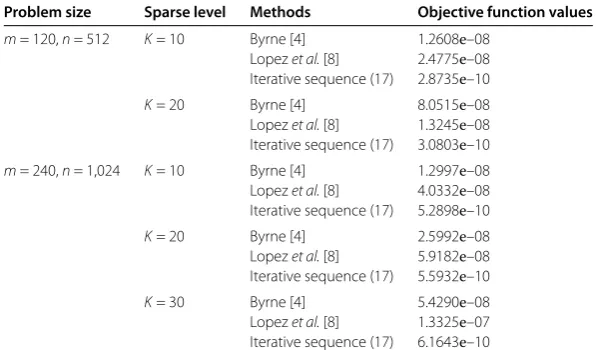
Table 1 The performance of the three iterative algorithms solving the LASSO in terms of the objective function values
Problem size Sparse level Methods Objective function values
m= 120,n= 512 K= 10 Byrne [4] 1.2608e–08
Lopezet al.[8] 2.4775e–08 Iterative sequence (17) 2.8735e–10
K= 20 Byrne [4] 8.0515e–08
Lopezet al.[8] 1.3245e–08 Iterative sequence (17) 3.0803e–10
m= 240,n= 1,024 K= 10 Byrne [4] 1.2997e–08
Lopezet al.[8] 4.0332e–08 Iterative sequence (17) 5.2898e–10
K= 20 Byrne [4] 2.5992e–08
Lopezet al.[8] 5.9182e–08 Iterative sequence (17) 5.5932e–10
K= 30 Byrne [4] 5.4290e–08
Lopezet al.[8] 1.3325e–07 Iterative sequence (17) 6.1643e–10
Figure 2 The random sparse signal is recovered by Byrne [4].
Figure 3 The random sparse signal is recovered by Lopezet al.[8].
the given criteria. We can see from Table that our proposed iterative sequence reaches smaller values than the other two methods.
5.2 Two MSSFP problems
In this part, we present two examples of MSSFP and compare several existing iterative algorithms.
() Self-adaptive methods proposed by Zhao and Yang [].
() Cyclic iterative algorithm and simultaneous iterative algorithm with self-adaptive step size proposed by Wenet al.[].
() Our proposed iterative algorithms () and ().
In what follows, we define a vector e={, , . . . , }T and chooseρk = . andρk= . in the iterative sequences () and (), respectively. The iterative parameters in Zhao and Yang [] and Wenet al.[] were chosen as suggested by the authors.
Example . The MSSFP withCi={x∈Rn|x–di≤ri},i= , , . . . ,t, andQj={y∈
Rm|L
j≤y≤Uj},j= , , . . . ,r. LetA= (aij)m×nandaij∈[, ], wheredi∈[e, e],ri∈
[, ],Lj∈[e, e] andUj∈[e, e] are all generated randomly.
Example . The MSSFP with Ci ={x ∈Rn|x–di ≤ri}, i = , , . . . ,t, and Qj =
{y∈Rm|
yTBjy+b
T
j y+cj≤},j= , , . . . ,r, wheredi∈(e, e),ri∈(, ), bj∈
(–e, –e),cj∈(–, –), and all elements of the matrixBj(in the interval (, ))
are all generated randomly. The matrixAis the same as in Example ..
Table 2 Example 5.1 witht=r= 20,m= 60,n= 80
Methods Initial point δ= 10–5 δ= 10–6 δ= 10–7 δ= 10–8
k k k k
Zhao and Yang [17] e 311 433 539 629
100e 318 366 447 527
–100e 214 276 321 353
Cyclic of Wenet al.[18] e 119 145 170 196
100e 139 169 198 227
–100e 128 156 183 210
Simultaneous of Wenet al.[18] e 1,743 2,431 3,135 3,841
100e 1,991 2,724 3,473 4,226
–100e 1,819 2,589 3,354 4,131
Iterative sequence (7) e 494 613 725 834
100e 514 640 762 878
–100e 513 643 762 878
The number ofkis the iteration number when the objection functiong(x)of (3) satisfiesg(x)≤δfor some given smallδ.
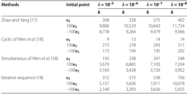
Table 3 Example 5.2 witht=r= 30,m= 50,n= 60
Methods Initial point δ= 10–5 δ= 10–6 δ= 10–7 δ= 10–8
k k k k
Zhao and Yang [17] e 268 328 375 402
100e 9,806 10,529 10,643 11,724
–100e 8,778 9,264 9,479 9,566
Cyclic of Wenet al.[18] e 9 13 14 14
100e 273 278 293 311
–100e 173 194 195 202
Simultaneous of Wenet al.[18] e 192 238 247 248
100e 5,679 6,865 7,103 7,334
–100e 3,163 3,428 3,726 3,952
Iterative sequence (18) e 312 515 538 756
100e 5,157 5,636 7,017 10,078
–100e 2,140 3,393 3,656 5,925
The numerical results obtained by the relaxed iterative algorithm of Zhao and Yang [17], Wenet al.[18] and iterative sequence (18), wherekis the same as in Table 2.
It follows from Table and Table that we find the (relaxed) cyclic iterative sequence of Wenet al.[] converges with less iteration numbers than the other iterative sequences. Because of the (relaxed) cyclic iteration method, an updated iteration number after all constrained sets is calculated. Our new proposed iterative sequence () and relaxed itera-tive sequence () are better than the simultaneous iteraitera-tive sequence of Wenet al.[] in Example . and Zhao and Yang [] in Example ., respectively. From a practical point of view, it is better to use all the proposed methods to solve a desired problem in practice and decide to choose a suitable one.
6 Conclusions
with the new step size and proved its convergence. Numerical experiments in the LASSO problem and two MSSFP examples showed that our proposed methods perform better than other methods in some ways.
Competing interests
The authors declare that they have no competing interests.
Authors’ contributions
All authors contributed equally and significantly in writing this article. All authors read and approved the final manuscript.
Author details
1Department of Mathematics, Nanchang University, Nanchang, 330031, P.R. China.2School of Information Engineering,
Nanchang University, Nanchang, 330031, P.R. China.
Acknowledgements
The authors wish to thank the editor and referees for their helpful comments and suggestions. This work was also supported by the National Natural Science Foundation of China (11361042, 11071108, 11401293, 11461046) and the Natural Science Foundation of Jiangxi Province (20151BAB211010, 20142BAB211016, 20132BAB201001).
Received: 22 May 2015 Accepted: 24 September 2015 References
1. Censor, Y, Elfving, T, Kopf, N, Bortfeld, T: The multiple-sets split feasibility problem and its applications for inverse problems. Inverse Probl.21, 2071-2084 (2005)
2. Censor, Y, Elfving, T: A multiprojection algorithm using Bregman projections in a product space. Numer. Algorithms8, 221-239 (1994)
3. Byrne, C: Iterative oblique projection onto convex sets and the split feasibility problem. Inverse Probl.18, 441-453 (2002)
4. Byrne, C: A unified treatment of some iterative algorithms in signal processing and image reconstruction. Inverse Probl.20, 103-120 (2004)
5. Xu, HK: Iterative methods for the split feasibility problem in infinite dimensional Hilbert spaces. Inverse Probl.26, 105018 (2010)
6. Qu, B, Xiu, N: A note on the CQ algorithm for the split feasibility problem. Inverse Probl.21, 1655-1665 (2005) 7. Yang, Q: The relaxed CQ algorithm solving the split feasibility problem. Inverse Probl.20, 1261-1266 (2004) 8. Lopez, G, Martin-Marquez, V, Wang, F, Xu, HK: Solving the split feasibility problem without prior knowledge of matrix
norms. Inverse Probl.28, 085004 (2012)
9. Yang, Q: On variable-step relaxed projection algorithm for variational inequalities. J. Math. Anal. Appl.302, 166-179 (2005)
10. Xu, HK: A variable Krasnoselskii-Mann algorithm and the multiple-set split feasibility problem. Inverse Probl.22, 2021-2034 (2006)
11. Zhang, W, Han, D, Li, Z: A self-adaptive projection method for solving the multiple-sets split feasibility problem. Inverse Probl.25, 115001 (2009)
12. He, BS, He, XZ, Liu, HX, Wu, T: Self-adaptive projection method for co-coercive variational inequalities. Eur. J. Oper. Res.
196, 43-48 (2009)
13. Zhao, J, Yang, Q: Self-adaptive projection methods for the multiple-sets split feasibility problem. Inverse Probl.27, 035009 (2011)
14. Chen, Y, Guo, YS, Yu, YR, Chen, RD: Self-adaptive and relaxed self-adaptive projection methods for solving the multiple-set split feasibility problem. Abstr. Appl. Anal.2012, 958040 (2012)
15. Zhao, JL, Yang, QZ: Several acceleration schemes for solving the multiple-sets split feasibility problem. Linear Algebra Appl.437, 1648-1657 (2012)
16. Zhao, JL, Zhang, YJ, Yang, Q: Modified projection methods for the split feasibility problem and the multiple-sets split feasibility problem. Appl. Math. Comput.219, 1644-1653 (2012)
17. Zhao, JL, Yang, Q: A simple projection method for solving the multiple-sets split feasibility problem. Inverse Probl. Sci. Eng.21, 537-546 (2013)
18. Wen, M, Peng, JG, Tang, YC: A cyclic and simultaneous iterative method for solving the multiple-sets split feasibility problem. J. Optim. Theory Appl.166(3), 844-860 (2015)
19. Bauschke, HH, Combettes, PL: Convex Analysis and Monotone Operator Theory in Hilbert Spaces. Springer, London (2011)
![Figure 2 The random sparse signal is recovered by Byrne [4].](https://thumb-us.123doks.com/thumbv2/123dok_us/9619082.1944129/13.595.116.479.80.368/figure-random-sparse-signal-recovered-byrne.webp)