1
Antenna Beamforming and Power
Control for Ad Hoc Networks
RAM RAMANATHAN
BBN Technologies Cambridge, Massachusetts
1.1 INTRODUCTION
The physical layer underlying ad hoc networks has a number of parameters that can be controlled for improved performance. Such parameters include modulation, transmit power, spreading code, and antenna beams. By controlling these transceiver parameters adaptively, and in an intelligent manner, one can increase the capacity of the system tremendously.
This chapter addresses the question: how do we control the physical layer
pa-rameters for best performance? We consider two papa-rameters – transmit power, and
antenna beam direction – and present state-of-the-art methods for their control, and their results on the performance. While control of other parameters (such as mod-ulation, coding, etc.) can also yield benefits, we shall focus on antenna and power control as they have been the most studied, perhaps because they are intuitively the easiest to exploit. Further, as we shall examine in considerable detail later, power control and beamforming are highly synergistic. It is therefore useful to study these parameters jointly, as this chapter does.
The benefits of antenna beamforming include reduced interference due to the narrower beamwidth, longer range due to higher signal-to-noise ratio (by virtue of higher gain and lesser multipath), and improved resistance to jamming. The bene-fits of power control includes reduced interference and lower energy consumption. Beamforming and lower powers are also good for covertness (often referred to as low probability of detection (LPD)). In sum, using antenna and power control enables higher capacity due to increased spatial reuse, lower latency and better connectivity, longer battery lifetime, and better security.
Controlling antenna and transmit power judiciously is far from easy. Improper control may result in performance that is poorer than without such control. For instance, reducing the power too much may leave the network unconnected, or
ii
duce excessive delays. Further, directional transmissions introduce new hidden and exposed terminal problems which may cause a decrease in capacity if not addressed. Thus, while the use of directional communications and power control appears to have potential, a number of questions need to be answered: What techniques are required for power and beamforming control? What are the tradeoffs involved in such control? Do existing network- and link-layer protocols have to be changed drastically? Does the performance improvement depend on the kind of antennas used, or the granularity of power control? Is this kind of control feasible in practice, has it been demonstrated? What kinds of performance improvements are possible, and what has been shown?
This chapter presents an overview of the work done toward answering these and other such questions. The goal is to provide the reader with an understanding of the problems encountered in the exploitation of beamforming antennas and power control, solution approaches to these problems, and their performance benefits. It is targeted toward the mobile ad hoc networking protocol researcher, providing her the necessary background, design tools, ideas and insights for exploiting beamforming and power control at the medium access and network layers.
We note that this is not a chapter on the physical layer. Rather, it is on how higher layers such as the medium access control (MAC) and network layers can control the parameters of physical layer technologies. One can think of the details of the particular technology itself as a black-box that offers “knobs” for control by higher layers. Such a control may be provided, architecturally, by way of Application Program Interfaces (APIs) above the physical and the medium access layer. Use of such APIs facilitates a clean way of controlling the transceiver parameters without layering violations.
This is also not a chapter on power conservation. While battery savings may occur as a side benefit of interference-reducing mechanisms, that is not a focus. Rather, the focus is on using antenna and power control for increasing the capacity, reducing delay, and increasing the connectivity of ad hoc networks.
A typical ad hoc network needs a number of mechanisms at the link and network layers working in cohesion to provide data communications. The medium access control (MAC) module provides distributed access to the channel; neighbor discovery is responsible for identifying nodes within one hop; routing determines routes to destinations and the forwarding module uses this information for, say, hop-by-hop packet forwarding. The exact functions performed by these modules is obviously system- and protocol-specific. For instance, in some reactive (on-demand) protocols, there is no explicit neighbor discovery, but this is implicitly done as part of routing.
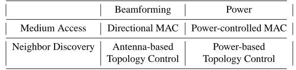
The majority of this chapter is thus devoted to a presentation of the problems in, and state-of-the-art solutions for, the 4 combinations shown in Table 1.1.
Table 1.1 The four different areas arising out of a combination of modules, and physical layer parameters, that are the subject of this chapter
Beamforming Power
Medium Access Directional MAC Power-controlled MAC
Neighbor Discovery Antenna-based Power-based Topology Control Topology Control
The rest of this chapter is organized as follows. We begin with a brief and very informal tutorial on beamforming antennas. Then, in section 1.3, we discuss medium access control, in particular, directional MAC, power-controlled MAC and the benefits of combining the two controls. In section 1.4, we discuss neighbor discovery, which results in a mechanism for topology control. We first discuss power-based topology control and then antenna-based topology control. Section 1.5 summarizes the chapter and overviews some open problems and interesting areas of research.
1.2 BEAMFORMING ANTENNAS
Of the two transceiver parameters that are the subject of this chapter, namely trans-mit power and beamforming antennas, transtrans-mit power control is easily understood. Beamforming antennas, however, are a complex and intriguing subject that is not very well understood by the typical ad hoc neworking researcher. We therefore de-vote this section to a brief tutorial on beamforming antennas. This is not intended to cover all aspects of this technology, nor do we cover it precisely or formally. Rather, the idea is to give the basics in an informal and intuitive fashion to equip the reader unfamiliar with this topic with just enough knowledge to understand the remainder of this chapter. Readers familiar with beamforming antennas may skip this section. Readers wishing to explore this field in detail are referred to [1] and the citations therein.
1.2.1 Antenna Concepts
iv
The gain of an antenna is an important concept, and is used to quantify the directionality of an antenna. The gain of an antenna in a particular direction
= is given [1] by
(1.1)
where
is the power density in the direction
, is the average power density over all directions, and
is the efficiency of the antenna which accounts for losses. Informally, gain measures the relative power in one direction compared to an omnidirectional antenna. Thus, the higher the gain, the more directional is the antenna. The peak gain is the maximum gain taken over all directions. When a single value is given for the gain of an antenna, it usually refers to the peak gain. Gain is often measured in unitless decibels (dBi), that is,
10! #"$&%
')( , where
')( is the absolute value of gain. An isotropic antenna has a gain of 0 dBi. The “i” following the “dB” stands for “isotropic”.
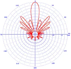
An antenna pattern is the specification of the gain values in each direction in space, sometimes depicted as projections on the azimuthal and elevation planes. It typically has a main lobe of peak gain and (smaller gain) side lobes. An example antenna pattern is shown in figure 1.2.1. As is common practice, we use the word beam as a synonym for “lobe”, especially when discussing antennas with multiple/controllable beams/lobes. A null is a direction of negative (in dBi) gain. For example, the pattern in figure 1.2.1 has a null at 30 degrees.
Fig. 1.1 An example “polar” pattern, with a main lobe at 0 degrees, and multiple sidelobes of varying gains.
same (you only have so much dough), the lobes have to balance each other out, that is, preserve the law of conservation of power.
A related concept is the antenna beamwidth. Typically, this means the “3 dB beam width”, which refers to the angle subtended by the two directions on either side of the direction of peak gain that are 3 dB down in gain. Gain and beamwidth are related. Typically, the more directional the antenna, higher the gain and smaller the beamwidth. However, two antennas with the same gain could have different beamwidths – for instance, the antenna with the smaller main lobe width may have more or larger sidelobes.
1.2.2 “Smart” Beamforming Antennas
The simplest way of improving the “intelligence” of antennas is to have multiple elements. The slight physical separation between elements results in signal diversity and can be used to counteract multipath effects. There are two well-known methods. In switched diversity the system continually switches between elements so as to always use the element with the best signal. While this reduces the negative effects of multipath fading, there is no increase in gain. In diversity combining, the phase error of multipath signals is corrected and the power combined to both reduce multipath and fading, as well as increase the gain.
The next step in sophistication involves incorporating more control in the way the signals from multiple elements (the antenna array) are used to provide increased gain, more beams and beam agility. Again, there are two main classes of techniques, as described below.
In switched beam systems, multiple fixed beams are formed by shifting the phase of each element’s signal by a predetermined amount (this is done by a beamforming
network), or simply by switching between several fixed directional antennas. The
transceiver can then choose between one or more beams/antennas for transmitting or receiving. While providing increased spatial reuse, switched beam systems cannot track moving nodes which therefore experience periods of lower gain as they move between beams.
In a steered beam system, the main lobe can be pointed virtually in any direc-tion, and often automatically using the received signal from the target. One may distinguish between two kinds of steered beam systems – dynamic phased arrays which maximizes the gain toward the target, and adaptive arrays which additionally minimize the gain (produce nulls) toward interfering sources. The former allows
beam steering, and the latter additionally provides adaptive beamforming.
In this paper, we consider switched beam and steered beam antennas, jointly referred to as a beamforming antenna.
1.2.3 Relevance for Ad Hoc Networks
vi
In this section, we argue that there do exist antenna techniques with suitable price and form-factor combinations.
Applications for ad hoc networking may be classified broadly into three categories: military, commercial outdoor, and commerical indoor, each with its own distinctive profile, and able to accommodate different antenna technologies.
Military networks, which are by far the most prevalent application of mobile ad hoc networks, contain a significant number of large nodes (such as tanks, airplanes). The size of these platforms makes the form factor of most antennas quite irrelevant. Further, each platform by itself is so expensive that the cost of even the most sophisti-cated antenna is dwarfed by comparison. Thus, beamforming antennas are extremely relevant to military networks.
Fixed ad hoc networks for commercial outdoor insfrastructure extend the reach of base stations using wireless repeaters organized into an ad hoc network. Packets are multi-hop routed through these repeater nodes with dynamic path selection. In some commercial approaches, the end-user terminals themselves serve as repeaters. Here steered beam approaches may be too expensive. However, switched beams using inexpensive beamforming networks such as the Butler matrix [2] are easily manufac-tured using inexpensive hybrid couplers etc. [1] making switched beamforming quite relevant.
The biggest deterrent to using beamforming antennas for networking small nodes such as PDAs and laptops within an indoor environment is the size. At 2.4 GHz, and the typical half-wavelength element spacing, an eight element cylindrical array would have a radius of about 8 cm, making it quite unwieldy. However, as the operating frequency continues to increase (already the IEEE 802.11a is working on wireless LANs in the 5 GHz band), the antenna sizes will shrink. At the 5.8 GHz ISM band, the 8-element cylindrical array will have a radius of only 3.3 cm, and at the 24 GHz ISM band, a mere 0.8 cm. Thus, the future looks bright for applying beamforming technology even to such applications.
Thus, while at first glance it may seem that ad hoc networks and beamforming antennas are not compatible, a more careful examination opens up a number of possibilities.
1.3 MEDIUM ACCESS CONTROL
The goal of the medium access control (MAC) is to enable efficient sharing of the common wireless channel between nodes that need access to it. In order to be efficient, the MAC typically needs to employ spatial reuse of the channel, that is, having as many simultaneous communications as possible.
Harnessing this potential, however, is non-trivial. Many MAC solutions tacitly assume homogeneous transmit power and/or omnidirectional transmissions. When these assumptions are violated, performance may deteriorate to below the perfor-mance when no control is used. We shall discuss these pitfalls in more detail later. For now, it suffices to say that techniques specifically targeted at supporting and exploiting power and beam control are required. Such techniques are the subject of this section.
Medium access control approaches may be broadly classified into two – contention-based and contention-free. For ad hoc networks, the most commonly considered contention-based approach is CSMA/CA (Carrier Sense Multiple Access with Col-lision Avoidance), and the most commonly considered contention-free approach is TDMA (Time Division Multiple Access). We shall survey adaptations of both CSMA/CA and TDMA, although focusing more on CSMA/CA because, being the basis for the IEEE 802.11 standard, it has received far greater attention.
We begin with a treatment of directional medium access control, and then survey power-controlled MAC. Finally, we consider MAC solutions that exploit both beam and power control.
1.3.1 Directional MAC
We first consider CSMA/CA. Protocols in the literature that are based on this ap-proach include MACAW [4], FAMA [5]. The IEEE 802.11 standard Distributed Coordination Function (DCF) is based on CSMA/CA and is a good example of this approach. We describe it briefly below. Details can be found in [6, 7].
The IEEE 802.11 MAC protocol The IEEE 802.11 DCF used up to four frames for each data packet transfer. A sender first transmits a Request-to-Send (RTS), and the receiver responds with a Clear-to-Send (CTS). Then the sender sends the DATA and finally the receiver completes the transaction with an Acknowledgment (ACK). Both RTS and CTS contain the proposed duration of the data frame. Nodes located in the vicinity of the sender and the receiver that overhear one or both of the RTS/CTS store the duration information in a network allocation vector (NAV), and defer transmission for the proposed duration. This is called virtual carrier sensing (VCS).
The IEEE 802.11 protocol uses a backoff mechanism to resolve contentions. Before initiating transmission, the sender first waits for a short time to see if the channel is idle (this “inter-frame spacing” is different for different kinds of frames). Then, the sender chooses a random backoff interval from a range [0,CW], where CW is the contention window. The sender then decrements the backoff counter once every “slot time”. When the backoff counter reaches 0, the sender transmits the frame. During this backoff stage, if a node senses the channel as busy, it freezes the backoff counter. When the channel is once again idle for a duration called DIFS (DCF Interframe Spacing), the node continues counting down from its previous (frozen) value.
viii
contention window is doubled upon each such event until it reaches a maximum threshold. Upon successful delivery of a packet, the contention window is reset to CW.
We now consider the problem of adapting CSMA/CA, and in particular, 802.11 to the directional regime. An obvious solution to the problem is to do exactly as in IEEE 802.11, but simply send all of the RTS/CTS/DATA/ACK packets directionally. Unfortunately, this has a number of problems. We discuss some of these problems below.
1.3.1.1 Problems with CSMA/CA when beamforming is used We present exam-ples of four kinds of problems due to directionality of transmission/reception. The scenarios are taken from [8] and [9].
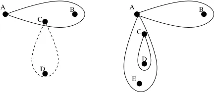
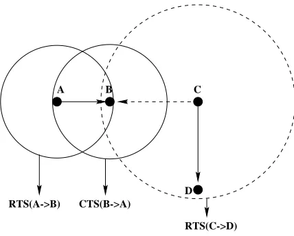
The first two examples are based on figure 1.2. In figure 1.2(left), * wants to send a packet to + , and, wants to send a packet to - . The RTS from * is sent omnidirectionally or directionally to+ , but is heard by, , and , is inhibited from sending even though it can do so without interfering with the transmission from* to
+ . We term this the directional exposed terminal.
E
A B
C
D
A B
C
D
Fig. 1.2 Examples when traditional CSMA/CA is insufficient when beamforming is em-ployed. In the example on the left, termed “directional exposed terminal”,. is prevented from sending when it can. In the example on the right, termed “loss in channel state”, there is a collision at D.
In figure 1.2(right), suppose* is sending a packet to+ after having initiated an RTS-CTS exchange. Neither the RTS nor the CTS is heard by, , which proceeds to initiate a transmission to- . The RTS-CTS exchange between, and- is directional and not heard by* , which, after completing its transmission to+ , now initiates a transmission to/ . The RTS from* to/ interferes with the data being received by
- from, . We refer to this situation as loss in channel state by node* .
For the next two examples, we refer to figure 1.3. The first of these examples is as follows. Assume all nodes in figure 1.3 when idle, are receiving using an omnidirectional beam which has an azimuthal gain of0
. Now, suppose+ transmits a directional RTS to 1 , and 1 responds with a directional CTS. Suppose node A is far enough from node F so as to not be able to hear this CTS. + begins DATA transmission to F, both nodes pointing at each other with gain
this DATA transmission. While this is in progress, suppose* wants to send to / . When it sends the RTS directionally toward/ (and it does so because it cannot sense anything), it interferes with the reception at1 . This can happen because beams of both1 and* are pointed toward each other. In other words, sender and receiver nodes with a combined gain of 2 0
may be out of range of each other, but within range with a combined range of34
(note that
is by definition greater than % ). We term this the directional hidden terminal problem1.
E
A
F
C
B
Fig. 1.3 Figure to illustrate “directional hidden terminal” and “deafness” (refer text)
For the final example, refer again to figure 1.3. Suppose+ initiates communication with/ and starts sending a DATA to/ . Further suppose that, is on a null for this transmission and so cannot hear these. While the+ -/ communication is ongoing,, wishes to send a DATA packet to+ , and so sends an RTS to+ . Since+ is beamformed in the direction of/ , it does not receive the RTS and so does not respond with a CTS. Node , , upon not receiving the CTS, retransmits the RTS. This goes on until the RTS retranmission limit is exceeded. This wastes network capacity in unproductive control packets. Furthermore, , increases its backoff interval on each attempt and thus unfairness is introduced. This problem has been termed deafness in [9].
In addition to all this, there are some aspects of CSMA/CA protocol design that don’t quite work when beamforming antennas are used. Consider the backoff scheme in IEEE 802.11 for example. This involves picking a random number of slots and counting down, freezing the count whenever the channel is busy. This is straightforward when there is only one beam that can be formed (omni), but is not so straightforward when beamforming is possible (steered or switched). While backing off, what beam should the node pick/form? Should it be omnidirectional, or should it continue to be beamformed in the direction of the intended transmission? If the former, the node misses the activity in the vicinity of the intended receiver. If the latter, then it may not be able to receive RTSs from nodes in other directions.
Last but not least, there is the issue of determining the direction in which the beam should be pointed to send to a target node, or in switched beams, which beam should be selected.
1This example does not apply to systems in which the beam automatically changes from omni to a
x
The examples outlined are by no means the only problems. However, they should have given the reader a flavor of the kinds of issues that researchers have grappled with in adapting CSMA/CA to beamformed transmissions. We now present a survey of research on solving these problems, under the informal umbrella of "directional CSMA/CA".
1.3.1.2 Directional CSMA/CA The examples above indicate that the RTS/CTS handshake as used in traditional CSMA/CA is insufficient to overcome the new “directional” hidden and exposed terminal problems. In general, as the number of nodes hearing the RTS/CTS increases, the severity of the exposed terminal prob-lem increases, and that of the hidden terminal probprob-lem decreases (the reader should examine the above examples again to grasp this intuition). Thus, one idea is to attempt to find an optimum point by exploring the various combinations of omnidi-rectional/directional RTS/CTS.
The other, largely orthogonal, approach to the problem is to introduce mechanisms that explicitly try and reduce the exposed or hidden terminal problems. For instance, an exposed terminal may violate the protocol rules and transmit anyway to get the spatial reuse.
These ideas, or a combination thereof, form the underlying rationale behind many of the schemes in the literature. A specific example is a simple scheme where nodes send omnidirectional RTS/CTS, but nodes never honor the NAV - i.e., they always
violate the virtual carrier sensing - and the RTS/CTS is used merely to assist in the
pointing of antennas for the subsequent DATA/ACK exchange and for power control. This was suggested as a simple baseline scheme in [8].
Ideas for determining the steering direction or beam selection include using the positions of the target node and reference node to derive the angle, using angle-of-arrival (AOA) facilities in steered (smart/array) antennas, etc. Directional MACs are generally agonstic as to which method is used, as long as the relative angle is obtained with reasonable accuracy. Note that it is the RTS direction that poses a challeng-ing problem – the CTS/DATA/ACK can use position information placed in, or the angle-of-arrival of, the RTS/CTS/DATA (respectively) for determining the sending direction. To determine the RTS direction in the first place, one may use angle-of-arrival from overheard packets, obtain position information from overheard pack-ets or (omnidirectional) beacons specifically used for this purpose, use piggybacked position information in routing control packets, or simply send the RTS omnidirec-tionally. Each of these techniques have their advantages and disadvantages. In the ensuing discussion, we focus more on the spatial reuse qualities of various schemes, relegating the mechanics of direction determination as a largely orthogonal issue.
With this background in mind, let us now examine the ideas studied in the litera-ture. We first consider the theme of omnidirectional/directional RTS/CTS, and then consider mechanisms for reducing collisions and increasing spatial reuse.
is heard only on one antenna, an RTS may be sent out all other antennas except that one. Two schemes are described, both of which use directional DATA/ACK and omnidirectional CTS, but differ in the choice of how the RTS is sent - omnidirec-tionally or direcomnidirec-tionally. Simulations done with a mesh topology show, as expected, a throughput improvement over 802.11 with omnidirectional antennas. The relative performance of the two schemes is topology dependent. While [10] was one of the early works on the problem and really kick-started this field, it makes a few assumptions that were later learnt to be unrealistic. For instance, it was assumed that the node can identify the antenna through which a packet was received, and that the omnidirectional antenna range is equal to the directional range.
The omnidirectional versus directional issue is examined more closely in [11]. Here, each node is assumed to have a switched beam antenna using a beamforming matrix. Two schemes are compared. In both, CTS, DATA, and ACK are sent direc-tionally. The difference is in the RTS – in one, called Di-RTS, it is sent directionally, and in the other, called omni-RTS it is sent omnidirectionally. Simulations reported show that the Di-RTS scheme outperforms the omni-RTS scheme significantly in all cases. The authors suggest that this is because the directional RTS’s generate less interference. Another way of looking at this is that the exposed terminal problem affects throughput more than the hidden terminal.
Both RTS and CTS are sent omnidirectionally in the scheme in [26]. The authors consider an ad hoc network with steered beam antennas. In order to alleviate the exposed terminal problem caused by the omnidirectionality of the RTS and CTS, the traditional backoff due to virtual carrier sensing is violated by using a shorter NAV for nodes not wanting to send to the source or destination of an ongoing communication. Thus, if a node C wanting to send to D hears an RTS from A to B, it will defer until the CTS from B to A is complete, and then will proceed to send an RTS to D even while A is sending DATA to B. Nodes A and B lock themselves into a tight directional transmit/ receive link during data transfer and are largely immune to the communication between C and D. Power control is also used to reduce the signature of the DATA/ACK. Performance improvements over 802.11 of up to 130% in a 25 node grid and up to 260% in a 225 node grid are reported, even without power control. The power control aspect of this paper will be addressed in section 1.3.2.1.
Omnidirectional RTS/CTS has the advantage that one need not know the position of the intended target. However, it cannot exploit the range advantage of directional antennas, that is, when two nodes can talk with each other only when one of them beamforms to get the additional gain.
xii
field, and deferring only if the intended direction is within a threshold (for error margin) of that direction.
The scheme using such a DNAV in [12] improves network capacity by a factor of 3 to 4 over 802.11 for a 100 node network. This scheme uses “cached directions” based on angle-of-arrival information from overheard packets. This is used to send the RTS directionally. If the cache is empty, or if more than four RTS transmissions don’t elicit a response, omnidirectional RTS is used. A hallmark of this work is the very comprehensive physical layer and antenna modeling that provides a high level of confidence in the results. The performance results in [9] indicate a throughput increase by a factor of about 2 over traditional IEEE 802.11, but the antenna gains used were only 10 dBi. An interesting insight, pointed out in [9], is that if the flows are “aligned”, directional transmissions perform much worse since packets from the same flow contend along the transmission direction.
There are a number of other works that consider directional CSMA/CA. In [13], signal strength information is used in lieu of position information to determine the angles. The novelty in [14] is in the use of an “Angle-SINR” table that keeps track of the communiation events and their directionality at any point in time. In [9], multi-hop RTS’s are proposed for sending DATA to a receiver when both sender and receiver need to beamform toward each other for successful data transfer. Finally, a host of issues in directional CSMA/CA, including a comparison between switched and steered beams is presented in [8].
Are there any lessons learnt from the research, and is there a convergence in thinking? While this is still a very young field, some insights are emerging. First, there is a bunch of “low hanging fruit” available for the taking – that is, even with simple modifications to CSMA/CA and moderate gain beams a capacity improvement of 2 to 4 is obtained. More sophisticated schemes should be able to increase this further. Second, as many packets should be sent directionally as possible (unless lack of position or other means forces one to use omnidirectional RTS). Third, a directional NAV and/or a short NAV is a good idea for exploiting the spatial reuse. Finally, and this will be discussed more in section 1.3.2.1, augmenting beamforming with power control makes significant difference to the performance.
1.3.1.3 Directional TDMA An alternative approach to channel access in ad hoc networks is the fixed, or contention-free approach. The most studied manifestation of this approach in ad hoc networks is as Time Division Multiple Access (TDMA). While TDMA has not been studied as much as CSMA/CA (at least in recent times), there is no evidence that this is due to any inherent demerits2of TDMA. Rather, the
relative simplicity of CSMA/CA and its adaptation by the IEEE 802.11 subcommittee is the likely cause of this relative imbalance in research.
2Some demerits are sensitivity to topological change, and unsuitability to highly bursty traffic. However,
In TDMA, time is divided into repeating frames. Each frame is divided into time
slots, which are at least approximately synchronized. Transmissions start and end
within slots. In a sufficiently spread out ad hoc network, slots can be reused by (adequately distant) nodes. Some researchers (e.g. [20]) refer to this specifically as
spatial reuse TDMA. In the reminder of this discussion, we use TDMA as a synonymn
for spatial-reuse TDMA.
The use of TDMA in ad hoc networks with omnidirectional antennas has been extensively studied. This includes theoretical studies based on a graph-coloring paradigm [15, 16, 17], and distributed procedures [18, 19]. Slots can be assigned to nodes – called broadcast scheduling (which is more suitable for broadcast packets), or link scheduling (which is more suitable for unicast packets). In both cases, the
activations (assignments of transmissions to a slot) must be made in a conflict-free
manner: that is, the activations must adhere to a a set of constraints. An example of a constraint is “Do not schedule concurrent transmissions at two nodes that are within 2 hops of each other”. Another example is “With all scheduled transmissions active, the Signal-to-Interference-Noise-Ratio (SINR) at all receivers must be above a certain threshold”.
The use of beamforming antennas in TDMA poses problems that are completely different than with CSMA/CA. This is a consequence of the entirely different ap-proach used for resolving contention – while CSMA/CA does this “on the fly” based on overheard control packets, TDMA does it apriori by coordinated decisions based on constraint information. In particular, the deafness and loss-in-state types of prob-lems cease to be an issue. Although hidden and exposed terminals exist, the problem is different since this is resolved while setting up the schedule (and factored in as part of the “constraints”).
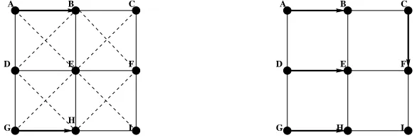
With beamforming antennas, what changes is the nature of constraints for con-current transmissions. For instance, consider figure 1.4. In the figure, two links are constrained if they are adjacent, or if there is a line from a transmitter to a receiver. For instance, in figure 1.4 (left)*657+ and-857/ are constrained, but*957+ and/6571 are not. Suppose all horizontal and vertical links need to be activated. The figure on the left shows interference constraints when omnidirectional tranmsis-sions are used and the figure on the right shows constraints when highly directional transmissions are used. With omnidirectional transmissions (left), many more links are constrained when compared to highly directional transmissions (right).
When scheduling, we need to ensure that there is no constraint line between a transmitter and its intended receiver. When omnidirectional antennas are used, only 2 links can be concurrently activated (figure 1.4 (left)), namely*:5;+ , and
5=< . However, with directional communications (figure 1.4 (right)), 4 links *>5?+ ,
-@5A/ ,
5B< , and,C5A1 can concurrently activated, giving a 100% increase in capacity.
xiv
Given an existing omnidirectional TDMA design, and thus an extant vehicle for translating constraints into dynamic schedules, it appears incrementally less complex to accommodate directional antennas. What is needed is to determine the new set of constraints accurately. We discuss ideas to do this by describing two representative works [20, 21].
I
A B C
D E F
G H I
A B C
D E F
G H
Fig. 1.4 Constraints, and activated links for a network with omnidirectional (left) and highly directional (right) beamforming. The reduction in constraints (indicated by solid or dashed lines) in the directional case allows four links to be simultaneoously activated compared to two in the omnidirectional case. Activated links are shown in bold
In [20], the authors study the performance of ad hoc networks with a TDMA MAC and two kinds of beamforming antennas – beam steering and adaptive beamforming. The algorithm used is a centralized one that uses two constraints: (1) in each slot links are activated such that the SINR is above a certain threshold; (2) a node can either transmit or receive one packet in a slot. The difference between directional and omnidirectional antennas is mostly in (1). With beamforming, interference is significantly reduced at many nodes, thereby increasing SINR, and allowing more simultaneous activations. Simulation results show that with beam steering for trans-mitting and adaptive beamforming for receiving, a capacity gain of about 980% over omnidirectional antennas is obtained.
1.3.2 Power-controlled MAC
Traditional versions of CSMA/CA, including IEEE 802.11, FAMA, MACAW, etc. assume that all nodes transmit all packets with the same power. However, this does not fully exploit the potential for spatial reuse. Spatial reuse using power control is possible at two levels: first, each node can be assigned a different maximum power that it must not exceed, but all packets from that node get sent with this power; second, within a given maximum power, a node modulates the individual powers of each packet – including control and DATA – so as to cause the least interference.
It is the second topic that is the subject of this section – the first problem of picking the right maximum power is addressed later in 1.4. We note that one can be done independent of the other and have their individual benefits.
We primarily consider CSMA/CA MACs here because, as with beamforming, most of the research has been done in this context. Further, we assume that all nodes only use omnidirectional transmissions. The combination of directional antennas and power control will be considered in section 1.3.2.1.
A simple idea is to send the RTS and CTS at the maximum power, and using their received signal strengths, reduce the power of the DATA and ACK to the minimum required. However, this does not affect spatial reuse because the number of other nodes that defer based on the RTS and CTS is not reduced, and thus, there is no improvement in spectral reuse3. Thus, in order to obtain spatial reuse we need to
send the RTS and CTS also at a reduced power. Ideally, this power should be just enough to reach the neighbors, and therefore might need to be different for different node pairs.
Unfortunately, CSMA/CA is inherently incompatible with such an approach. To see why, consider the example illustrated in figure 1.5. Consider two nodes* and
+ that are close to each other, and suppose that* wishes to send to+ . The CTS from+ to* uses a (low) power, sayD
$ which is less than the maximum possible powerDFE
G . Now, suppose another node
, that cannot hear the RTS/CTS exchange between* and+ wishes to send to a distant node- such that it has to useDFE
G . If+ is within range of, withDFE
G , then the RTS and the DATA from
, to- will collide with the DATA from* to+ .
In other words, the RTS/CTS exchange does not prevent hidden terminal problem when heterogenous power levels are used. In general, the control and data packets in a CSMA/CA regime must be transmitted with the largest power that any node can use [22], in order to guarantee collision-free floor acquisition. However, this brings us back to the original problem – sending only RTS/CTSs at the maximum power yields little additional benefit over no power control.
This dilemma has been addressed in [22, 23]. Both solutions make use of busy
tones for virtual carrier sensing, and utilize the RTS/CTS more as a way of negotiating
the correct power level for DATA. In a way, this is similar to the violation of the virtual carrier sensing described in the context of beamforming in section 1.3.1.2.
3In practice, depending upon the carrier sense threshold, one may see a slight improvement because nodes
xvi
RTS(C->D)
A B C
D RTS(A->B) CTS(B->A)
Fig. 1.5 Heterogeneous transmit powers resulting from power control causes problems for CSMA/CA. NodesH andI reduce power when sending RTS/CTS, which is not heard by. . When. transmits to a distant nodeJ it needs to use a high power, causing collision atI .
We describe the solution below, based on [22], and called Power Controlled Multiple Access (PCMA).
In PCMA, collision avoidance is generalized to power control. Unlike the “on/off” model of conventional CSMA/CA, PCMA uses a “bounded power” model using two main mechanisms:
1. A Request-Power-to-Send (RPTS) and Acceptable-Power-to-Send (APTS) handshake used to determine the minimum power that will result in a succesful transmission. The RPTS/APTS transmission occurs in the data channel.
2. Each active receiver advertises its noise tolerance, given its current received signal and noise levels. This is done using pulses in the busy tone channel, where the strength of the pulse indicates the tolerance to additional noise.
A sender node continuously monitors the busy tone channel to determine its power bound by measuring the maximum power received on the busy tone channel over a threshold time window. Then, using a backoff similar to (but not identical) traditional 802.11, the sender transmits an RPTS at a power level slightly below the bound.
The solution in [23] also uses busy tones to coordinate power control, but the tones here are continuous. Two busy tones are used: transmit busy tone, sent by an active transmitter, and a receive busy tone, sent by an active receiver. Different power levels are used for the tones by the transmitter and the receiver, and tuned appropriately.
Both [22] and [23] show significant performance gains from the respective methods using simulation. A throughput improvement by a factor of 2 over non-power controlled IEEE 802.11 is achieved using the mechanism in [22]. The approach of [23] is shown to provide approximately twice the peak channel utilization when compared to a non-power controlled dual busy tone technique, namely the one in [24]. While the above solutions manage to avoid collisions, they require the use of a second channel for busy tones. This implies a second transceiver since the busy tones and transmission/reception may need to happen simultaneously. Thus, this is not possible with the off-the-shelf 802.11 wireless cards, and indeed, one might argue that with two channels and two transceivers, non-power controlled 802.11 might itself exhibit close to factor-of-2 performance gains. From a practical viewpoint, the problem that would be of most interest is a power-controlled CSMA/CA with a single
channel and transceiver. As far as we know, this is an open problem. However, a
trivial solution to this problem is to not address the collisions, resolving them by means of backoffs and retransmissions. Our experience, reported in [8], and in other unpublished research is that one can still get substantial gains in performance.
Thus far we have considered power control in the context of CSMA/CA. One of the few works that addresses power control in the TDMA context is in [25]. The authors present a two-phase algorithm that searches for an admissible set of users in a slot, along with their transmission power. In the first phase, a scheduling algorithm is used to eliminate “strong” or “primary” constraints – for example, a node cannot simultaneously transmit and receive. In the second phase, a distributed algorithm is executed to control the admissible set of powers that could be used by nodes scheduled in phase 1. As in the case of TDMA with beamforming, power computation simply translates into a new set of constraints that need to be accommodated. In this case, the constraint is that the powers should be such that the SINR at every receiver must be greater than a given threshold.
1.3.2.1 Power-controlled Directional MAC Although beam and power control by themselves can improve spatial reuse considerably, it is when both are employed simultaneously that the full potential is realized. Figure 1.6 illustrates this very informally by comparing the four combinations – no power or beamforming control, only power control, only beamforming, and both. Ignoring a number of details such as sidelobes, one can take the ratio of the areas occupied by two schemes as a measure of the relative spatial reuse. Suppose that a node wants to send to a node that is at half the range of its maximum power (top left). With power control (top right), the relative area decreases by a factor of KMLON
KQP!LRST
N
or 4. With only beamforming with a beamwidth of 10 degrees (bottom left), energy is redirected but the same energy is emanated. Assuming, and because of, UWV propagation, the energy interferes with less area than without power control or beamforming but still interferes significantly. Specifically, the range is
YX#ZM[\]^[
$
xviii
power control or beamforming, which is 50% better than with only power control. When both power and beamforming control are used (bottom right), the area occupied is approximately $_%
`a
%
cb
U
\
3
S , or a reduction in the area by a factor of 144!
Area = A/144
r r/2
10 degrees
No power or beamforming control
Only power control
Only
beamforming Both powercontrol and
beamforming
Area = A/6
Area = A Area = A/4
Fig. 1.6 A rough comparison of relative interference reduction potential with power control, beamforming, and both together. Assuming a beamwidth of 10 degrees anddfe propagation, and many simplifying assumptions, the area of interference is reduced by a factor of 4 with power control only, a factor of 6 with beamforming only, and a dramatic 144 with both together.
0 50 100 150 200 250 300
10 20 30 40 50 60 70 80 90 100 110 120
Delay-ms
g
Density
Delay-ms vs Density for various Gain; 40 nodes; NumAnt=1 ’Gain=0’ ’Gain=10’ ’Gain=14’ ’Gain=20’ ’Gain=26’
0 50 100 150 200 250 300
10 20 30 40 50 60 70 80 90 100 110 120
Delay-ms
g
Density
Delay-ms vs Density for various Gain; 40 nodes; NumAnt=1 ’Gain=0’ ’Gain=10’ ’Gain=14’ ’Gain=20’ ’Gain=26’
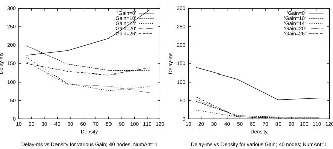
Fig. 1.7 Performance of beamforming without (left) and with (right) power control: 40 node stationary ad hoc network with steered beams.
Because of the large packet buffers used, packets are delayed rather than dropped, and therefore the delay metric is a better indicator of performance here [8]. We note that without power control (left) there is a factor of 2 to 3 reduction in delay, whereas with power control (right), there is a factor of about 28 reduction in delay.
We now summarize the results from [26]. As mentioned earlier, in the protocol proposed here, RTS and CTS are sent using omnidirectional antenna, and a short NAV is used to mitigate the exposed terminal problem. In this context, the authors study two power control schemes – global and local. In both cases, power control is applied only to the DATA/ACK packets. In global power control (GPC), the DATA/ACK transmitter power is reduced to the same level for all nodes, in particular, to a value
h
Di whereDFi is the transmitter power of RTS/CTS. In the local power control (LPC) scheme, the transmit power is set for each transmission so that the SNR across the link is a predetermined value. This is done by using the values of the received RTS/CTS power levels to compute how much power reduction is required.
xx
1.4 NEIGHBOR DISCOVERY: TOPOLOGY CONTROL
In the previous section, we studied the issues related to the spatial-reuse of spectrum. In this section, we consider the other dimension, namely communication range, and relatedly, connectivity control opportunities provided by antenna beam and power control.
The goal of neighbor discovery at each node is to determine the set of other nodes within direct communication range (within one hop). Neighbor discovery is an inherent part of most proactive protocols and uses a technique called beaconing to advertise itself and discover other nodes. In some reactive protocols, there is no explicit neighbor discovery. However, the process of building on-demand routes using route queries essentially discovers neighbors (that are in many cases cached for later use). One might therefore consider neighbor discovery as an implicit part of reactive protocols. Our description in this section is in the context of a proactive protocol, but we note that many of the ideas and issues are applicable in a modified form to reactive protocols as well.
The set of potential neighbors depends upon "uncontrollable" factors such as mobility, weather, noise, interference etc. as well as "controllable" ones such as transmit power and antenna direction. For instance, increasing the transmit power of beacons typically increases the number of neighbors. Similarly, depending upon whether the beaconing employs beamforming at one or both ends, different neighbors can be discovered.
The topology of the network is union ofj
, wherej
is the set of links discovered by a nodek. More generally, the topology of a network is the set of communication links used explicitly or implicitly by a routing mechanism [27]. Controlling the neighborhood of each node using power and beamforming obviously also controls the topology. This leads us to the notion of topology control, which is the problem of controlling the topology of the network to the desired form by changing the radio parameters – in this chapter, we only consider transmit power and antenna beam.
Why do we need topology control? Simply because the wrong topology can con-siderably reduce the effective capacity, increase the latency, and reduce the robustness of the network. For instance, if the topology is too sparse, there is a danger of loss in connectivity, and higher chances of congestion at a single node. On the other hand, a dense topology often implies reduced spatial reuse and increased battery consump-tion. Further, routing protocols might incur too much overhead in maintaining the topology, and this may overwhelm the routing process.
We observe that topology control can by accomplished in two ways:
l
Restrict the parameters to physically discover only some of the potential neigh-bors. We call this physical topology control.
l
Given a set of discovered neighbors, filter or refer only a subset of these neighbors to the routing process. We call this routing topology control.
topology control. Both techniques can be used for controlling the set of links seen by routing. The techniques are orthogonal, and thus, one can employ both physical and routing topology control to control the topology at two levels. In this chapter, we study only physical topology control. Unless explicitly mentioned, the term "topology control" will mean physical topology control.
In the next subsection, we shall discuss topology control based on power adjust-ment. The basic problem here is how to pick the right range for each node to balance connectivity, energy and spatial reuse. Following that, we shall discuss topology control based on antenna beam pointing. The issue here is less about which nodes to pick4but how to form neighbors when one or both have to beamform toward the
other.
1.4.1 Power-based Topology Control
The generalized problem of power-based5topology control (recall that we are con-sidering on physical topology control in this chapter) is as follows [29, 27]: Given an ad hoc network, determine and adaptively adjust the transmit power of each node in the network so as to meet a given minimization objective and adhere to a given
connectivity constraint.
The above is a generalized definition and subsumes a number of specific prob-lems depending upon what is considered for the minimization objective and the connectivity constraint. Possibilities include:
l
Minimization objectives. Maximum power, average power, maximum degree,
average degree, maximum diameter, etc.
l
Connectivity constraints. Connectivity, biconnectivity, etc.
An example of a specific topology control problem is one of dynamically adjusting transmit powers such that the maximum power used is minimized while keeping the network biconnected. This was first studied in [27]. Clearly, a number of other combinations are possible.
There is a further dimension to the problem relating to the dynamism of topology control. That is, just as many other distributed control problems, one can consider the static version of the problem, or consider the dynamic version. In the static version, global topological information is available, the computation is “one-time” only, and it can use a centralized solution. In the dynamic version, only local information is available, the computation is continuous, and typically requires a distributed algorithm. Although the dynamic version is more useful for mobile ad hoc networks, a study of the static version gives valuable insight, is useful to define the upper bound on performance, has some applicability to stationary ad hoc
4Because in this case, acquiring distant nodes as neighbors does not impact the spatial reuse nearly as
much since transmissions are directional.
xxii
networks such as commercial mesh-based broadband wireless solutions, and is simple to understand.
In this subsection, we first examine the static version of the problem, and examine some algorithmic issues. We shall then consider the dynamic version and survey some decentralized and distributed approaches.
1.4.1.1 Static Topology Control We first introduce some terminology that will make the subsequent discussion less ambiguous.
First, an ad hoc network is represented as M = (N, L), where N is a set of nodes and L : N5 (mon% ,mpn% ) is a set of coordinates on the plane denoting the locations of the nodes.
The least-power functionq
gives the minimum power needed to communicate a distance of
. The function q
is dependent upon the propagation loss and the receiver sensitivity, and essentially maps from range to power (see [27] for details).
Using these, a graph theoretic representation is used as follows. Given a multihop wireless network M = (N, L), a transmit power functionr , and a least-power function
q , the induced graph is represented as G = (V, E), where V is a set of vertices corresponding to nodes in N, and E is a set of undirected6edges such thatYsFOtQ u
E if and only ifr
sv w
q
sxytz y , andr
tz w q YsFOtQ O .
We use standard graph-theoretic terminology from [30]. In particular, a graph is said to be k-vertex/edge-connected if and only if there are{ vertex/edge-disjoint paths between every pair of vertices. Note that if a graph is{ -vertex connected, then it is also{ -edge connected, but the converse is not true. For this reason, and because vertex connectivity is important for resilience to node failures and hotspots, we shall consider only vertex connectivity. We shall omit the word “vertex” for brevity. Thus, if { is 1, the graph is connected, and if { is 2, it is biconnected. The degree of a vertex is the number of edges incident on that vertex. We only consider undirected graphs, that is, all edge-relations on vertex pairs are symmetric.
Let us now consider a specific topology control problem, namely the one consid-ered in [27]. In this problem, the constraint is 1-connectivity, and the objective is minimization of maximum power. Formally,
Definition 1.4.1 Problem Connected MinMax Power (C-MMP). Given an M =
(N, L), and a least-power functionq , find a per-node minimal assignment of transmit powersr : N 5|m
n , such that the induced graph of (M,
q ,r ) is connected, and MAX}#~
r
Ys O
is a minimum.
An algorithm, called CONNECT, for this problem is given in the box below. It is a simple “greedy” algorithm, similar to the minimum cost spanning tree algorithm. It works by iteratively merging connected components until there is just one. Initially,
6An alternate, and arguably superior representation would use directed edges to include unidirectional
each node is its own component. Node pairs are selected in non-decreasing order of their mutual distance. If the nodes are in different components, then the transmit power of each is increased to be able to just reach the other. This is done until the network is connected. The description assumes for simplicity that network connectivity can be achieved without exceeding the maximum possible transmission powers. However, the algorithm can be easily modified to return a failure indication if this is not true.
Algorithm CONNECT
Input: (1) Multihop wireless network M = (N, L) (2)
Least-power functionq
Output: Power levelsr for each node that induces a connected
graph
begin
1. sort node pairs in non-decreasing order of mutual distance 2. initialize clusters, one per node
3. for each (u,v) in sorted order do
4. if cluster(u)
cluster(v)
5. r
Ys =r
tz =q
k_ f_v sxytz y
6. merge cluster(u) with cluster(v)
7. if number of clusters is 1
then end
8. perNodeMinimalize(M,q ,r , 1)
end
While this produces a minimum maximum power, it leaves some scope for reduc-ing the powers of some nodes without affectreduc-ing the connectivity. Line 8 in algorithm CONNECT is a procedure that exploits the presence of “side-effect edges” to mini-malize the power of each node resulting in a reduced average power. The details of this procedure can be found in [27].
This algorithm is provably optimal [27]. Algorithms for related problems, for example, the Biconnected Minimum Maximum Power (B-MMP), the Connected
Minimum Average Power (C-MAP) and the Connected Minimum Maximum Degree
(C-MMD) are of a similar flavor. Algorithms for these problems are given in [29]. However, unlike the C-MMP, not all of them are amenable to optimal solutions. The algorithm for B-MMP is provably optimal [27], but C-MAP has been proven to be NP-complete in a variety of settings [31, 32], making it highly unlikely that there is a polynomial-time optimal solution.
xxiv
Fig. 1.8 Uncontrolled network topology (left), connected topology using C-MMP solution (middle), and biconnected topology using B-MMP solution (right).
The algorithmic aspects of topology control are studied thoroughly in [33]. There a general approach leading to an optimum polynomial-time algorithm is presented for minimizing maximum power for a class of graph properties called monotone properties. A propertyD is monotone if the property continues to hold even when the powers assigned to some nodes are increased while the powers assigned to other nodes remain unchanged. For example, k-connectivity is monotone. Thus, the paper generalizes the results of [27] to hold for any k-connectivity constraint. They also give an approximation algorithm for the C-MAP problem that has a constant-times-optimum performance guarantee.
1.4.1.2 Dynamic Topology Control For dynamic networks, there are two ap-proaches to doing topology control.
l
Fully Distributed. Nodes only know local information. All nodes execute the
same (distributed) algorithm to produce the result.
l
Decentralized. All nodes have the global topology information through a
flooded exchange, and run the same algorithm to produce the same result, after which each node uses the part of the result that pertains to itself. This is similar to the way the traditional link-state routing protocol works.
A “zero overhead” distributed algorithm called Local Information No Topology (LINT) is described in [27]. In LINT, a node is configured with three parameters – the “desired” node degree
, a high threshold on the node degree
, and a low threshold
. Periodically, the node checks the number of active neighbors (degree) in its neighbor table (built by the routing mechanism). If the degree is greater than
, the node reduces its operational power. If the degree is less than
, the node increases its operational power. If neither is true, no action is taken. The magnitude of the power change is a function of desired degree
and current degree . In particular, the further apart
and
In [34], the concepts of a relay region and enclosure are used to select neighbors. A relay region for a node pair
k
U is the region such that, for any node in that region, it is more efficient for ank5 transmission to be relayed throughU than be sent directly. An enclosure for a nodek is computed based on the relay regions of
k
for each neighbor ofk. Intuitively, the enclosure is a region beyond which it is not power-efficient to have neighbors. One of the key results is that if every node maintains communication links with the nodes in its enclosure, the network is strongly connected. The authors provide a distributed algorithm based on this that yields strong connectivity.
In [35], a cone-based distributed algorithm is described. A node continues to grow its power until its neighbor set is big enough such that, for any cone with angle there is at least one neighbor or until the node hits the maximum allowable power. They provide simulation results that outperform the algorithm in [34] in the scenarios studied.
The decentralized approach is inherently more overhead-intensive, and less re-sponsive to changes. On the other hand, it allows for direct execution of the static algorithms. A decentralized topology control algorithm is described in [29]. The execution of that algorithm can be perceived as “punctuated equilibrium”, with events happening at globally synchronized periodic intervals (only rough synchronization is required, as might be provided by a GPS clock). At these topology reformation
moments (TRM), local state7is flooded, all nodes collect the individual local states to
form the current snapshot of the global topology, execute a heuristic (e.g. algorithm CONNECT), and use the result for itself as the new power. Until the next TRM, this new set of powers is used.
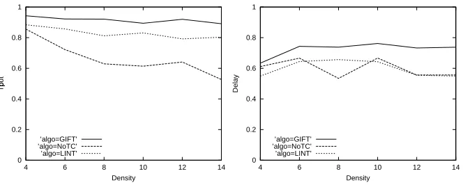
In [29], the decentralized solution to B-MMP (called GIFT for “Global Informa-tion Full Topology”) is compared with the Local InformaInforma-tion No Topology (LINT) algorithm, and to the performance when no topology control is employed. We reproduce those results in figure 1.9. All results reported here are for 60 nodes.
We note from figure 1.9 that the decentralized algorithm yields the best throughput. The throughput at density 14 is about 11% better than that of LINT, and about 71% better than no topology control. However, the delay is also slightly higher, about 27% more than LINT. The increased delay is a result of being less densely connected (giving rise to larger number of hops between node pairs).
Although it appears wasteful, the decentralized approach exploits the fact that after the powers are set the first time, one can have considerable interval between resets – that is, the TRMs can be fairly widely spaced apart. For instance, in the results discussed in the above paragraph, a 20 second interval was used. With this, the decentralized approach handily outperforms the LINT distributed algorithm for mobile networks, yet only uses about 0.5% of the capacity of a 2 Mbps transceiver. Thus, this is a simple yet scalable approach for at least non-highly-mobile ad hoc network applications.
xxvi
0 0.2 0.4 0.6 0.8 1
4 6 8 10 12 14
Tput
Density
Tput vs Density for various nbrMax; 60 nodes; Mobility=0.001, VC=N, LST=T ’algo=GIFT’
’algo=NoTC’ ’algo=LINT’
0 0.2 0.4 0.6 0.8 1
4 6 8 10 12 14
Delay
Density
Delay vs Density for various nbrMax; 60 nodes; Mobility=0.001, VC=N, LST=T ’algo=GIFT’
’algo=NoTC’ ’algo=LINT’
Fig. 1.9 A comparison of a decentralized algorithm (GIFT) and a distributed algorithm (LINT) with a no-topology-control (NoTC) in a 60 node mobile ad hoc network.
1.4.2 Topology Control using Beamforming Antennas
Transmitter beamforming provides additional gain in the direction that the packet is sent. Likewise, receiver beamforming provides additional gain in the direction from which a packet is received. These additional gains typically provide a significant increase in the range at which neighbors can be acquired. Moreover, which nodes can be neighbors depends upon whether none, one or both of the nodes beamform. Orthogonally, other mechanisms for increasing the processing gain along the direction of communication also influence the ability to form neighbors.
Conventional neighbor discovery techniques such as in in [36, 37] assume the presence of omnidirectional antennas, and are not sufficient to enable discovery of neighbors with beamforming. Thus, one problem is: How do we discover neighbors
using beamforming? While the problem is one of neighbor discovery, it is directly
related to topology control because differing capabilities in discovering neighbors leads to differences in the way topology control can be effected.
Once neighbors have been discovered, they have to be “maintained”. Such mainte-nance typically uses periodic transmissions of beacons, non receipt of which indicates that the link has gone down. Unlike broadcast beaconing in omnidirectional networks, where a single beacon suffices for all directions, we now may need multiple beacons: one for each direction or neighbor8. Thus, we are led to the next problem: How do we pick and choose the potential neighbors so as to get the desired topology? This may
be thought of as a dynamic degree-constrained network design problem. Very little work has been done on this, and therefore we only discuss the discovery problem in the remainder of this subsection.
8Note that we cannot use omnidirectional beacons because their range may be considerably less and cannot
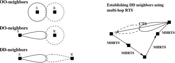
A neighbor relationship may be specified as
(
L
where
( is the beamform of the sender, and
L
is the beamform of the receiver. We consider two possibilities for
( and
L
: Omni (O) and Directional (D). Thus, we have four kinds of neighbors -OO, DO, DD, OD. This terminology was first used in [9]. The OO-neighbors can be discovered using traditional beaconing. Doing OD-neighbor discovery is harder than doing DO, and does not yield additional range or other benefits. Thus, we shall examine only two types in greater detail here: DO and DD. Figure 1.10 (left) illustrates OO, DO and DD neighbors.
We first consider DO-discovery. A key issue here is to know which direction a node * must point to in order to send to a node + . There are two ways of doing this. If+ is equipped with a smart antenna, it can eavesdrop on * ’s transmissions and compute the Angle-of-Arrival (AOA). Another method is to use relayed position information. If a link-state protocol is used, such position information becomes automatically available if current position is included in each update. Alternatively, one may use efficient position dissemination techniques, as in [38, 39]. Using one’s own position and the neighbor’s position, the direction is easily computed. Assume that* knows the direction of+ using one of these, or other techniques. Then DO-discovery is fairly simple:* beamforms towards+ and sends a beacon. We assume that nodes are receiving in omnidirectional mode when not active. Thus, if the gain is sufficient,then+ receives the beacon. The beacon contains* ’s position. + uses that information to beamform toward* and send a beacon, enabling DO neighbor discovery.
DD-discovery is more complicated, especially in a system that uses CSMA/CA at the MAC layer. In addition to the direction issue, which may be addressed in the same manner as for DO, a problem here is that the receiver must be beamformed in the direction of the sender at the precise time the beacon is sent. This is a problem not just for discovery, but for every single data packet transfer – although in a TDMA system, scheduling the pointing could solve the data transfer problem.
multi-hop RTS
MHRTS
MHRTS MHRTS
MHRTS
CTS
S R
S R
S R
OO-neighbors
DO-neighbors
DD-neighbors
Establishing DD neighbors using
Fig. 1.10 Left: OO, DO and DD neighbors. Solid lines indicate transmitter beamforming, dashed lines indicate receiver beamforming. DO has longer range than OO, and DD has longer range than DO. Right: Illustration of multi-hop RTS for establishing DD neighbors.
xxviii
rendezvous packet contains* ’s position and the exact time at which* expects+ to point toward* based on the position. Upon receipt of the rendezvous packet, and at the scheduled time,* and+ can point to each other and try sending beacons to see if they can be DD-neighbors.
In a CSMA/CA based system, a multi-hop RTS may be used in place of a separate rendezvous packet. That is, when the beacon reaches the MAC layer, the MAC protocol determines that this is not a DO or OO neighbor and source-routes the RTS multi-hop to the receiver. During this time,* remains beamformed in the direction of+ . Upon receipt of the RTS, which contains* ’s position, + beamforms toward
* and sends a CTS. If they can be DD-neighbors, then the CTS will reach* and* can directly send the DATA (in this case the beacon). Such a multi-hop RTS scheme is described in [9], and further implementation details may be found there.
Clearly, this approach will only work if the network is connected using only DO and OO links. What if it is not? This is a hard problem. However, if another physical layer parameter, namely spreading gain were controllable, one can trade data rate for increased processing gain (and hence range) just for the RTS, and use that to bootstrap the pointing.
What do DO and DD discovery give us? They essentially provide range extension which in turn provides richer connectivity and a smaller average number of hops. Both of these are beneficial for the performance, but not under all circumstances. In the remainder of this section, we study some performance implications of range extension using beamforming antennas.
In [9] two protocols called DMAC and MMAC are compared. DMAC is a CSMA/CA based protocol that uses a directional NAV table, as described in sec-tion 1.3.1.2. DMAC only implements OO and DO modes. MMAC is an en-hancement of DMAC with multi-hop RTS, which enables the DD mode. Thus, in DMAC, a packet may have to travel multiple hops, each of which involves an RTS/CTS/DATA/ACK exchange whereas in MMAC, the packet may travel only one hop which involves a single MHRTS/CTS/DATA/ACK exchange. Using beamwidth of 45 degrees and a DD-range of about 900 meters when compared to 250 meters for OO and a 25 node random network with random flows, the simulation results show that MMAC outperforms DMAC by a factor of up to 2.5. This clearly indicates the power of longer range transmissions to increase the capacity. MMAC also reduces the end-to-end delay by about 15%. The number is not very high because the queues saturate and packets are dropped (delay is only calculated for delivered packets). Further, the higher failure probability of multi-hop RTS in MMAC causes more time-outs and retransmissions, thereby offsetting some of the reduction in average packet latency.
In [8], the effect of range extension is studied using a model of switched beam antennas. A beacon is sent out on each of beams. Since these beacons travel farther than omni beacons, longer range neighbors and a richer topology are possible. The comparison is between OO- and DO-based topologies. The number of beams