17Giancoli Ch 17 E Potential

(1)

473

C

H

A

P

T

E

R

Electric Potential

We are used to voltage in our lives—a 12-volt car battery, 110 V or 220 V at home, 1.5-volt flashlight batteries, and so on. Here we see displayed the voltage produced across a human heart, known as an electrocardiogram. Voltage is the same as electric potential difference between two points. Electric potential is defined as the potential energy per unit charge.

We discuss voltage and its relation to electric field, as well as electric energy storage, capacitors, and applications including the ECG shown here, binary numbers and digital electronics, TV and computer monitors, and digital TV.

CHAPTER-OPENING QUESTION—Guess now!

When two positively charged small spheres are pushed toward each other, what happens to their potential energy?

(a) It remains unchanged. (b) It decreases.

(c) It increases.

(d) There is no potential energy in this situation.

W

e saw in Chapter 6 that the concept of energy was extremely valuable

in dealing with the subject of mechanics. For one thing, energy is a conserved quantity and is thus an important tool for understanding nature. Furthermore, we saw that many Problems could be solved using the energy concept even though a detailed knowledge of the forces involved was not possible, or when a calculation involving Newton’s laws would have been too difficult.

(2)

17–1

Electric Potential Energy and

Potential Difference

Electric Potential Energy

To apply conservation of energy, we need to define electric potential energy as we did for other types of potential energy. As we saw in Chapter 6, potential energy can be defined only for a conservative force. The work done by a conservative force in moving an object between any two positions is independent of the path

taken. The electrostatic force between any two charges (Eq. 16–1, )

is conservative because the dependence on position is just like the gravitational force (Eq. 5–4), which is conservative. Hence we can define potential energy PE for the electrostatic force.

We saw in Chapter 6 that the change in potential energy between any two points, a and b, equals the negative of the work done by the conservative force on an object as it moves from point a to point b:

Thus we define the change in electric potential energy, when a

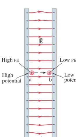
point charge qmoves from some point a to another point b, as the negative of the work done by the electric force on the charge as it moves from point a to point b. For example, consider the electric field between two equally but oppositely charged parallel plates; we assume their separation is small compared to their width and height, so the field will be uniform over most of the region, Fig. 17–1. Now con-sider a tiny positive point charge qplaced at the point “a” very near the positive plate as shown. This charge qis so small that it has no effect on If this charge qat point a is released, the electric force will do work on the charge and accelerate it toward the negative plate. The work Wdone by the electric field Eto move the charge a distance dis (using Eq. 16–5, )

.

The change in electric potential energy equals the negative of the work done by the electric force:

(17;1)

for this case of uniform electric field In the case illustrated, the potential energy decreases ( is negative); and as the charged particle accelerates from point a to point b in Fig. 17–1, the particle’s kinetic energy KEincreases—by an equal amount. In accord with the conservation of energy, electric potential energy is transformed into kinetic energy, and the total energy is conserved. Note that the positive charge qhas its greatest potential energy at point a, near the positive plate.†_{The reverse is true for a negative charge: its potential energy is greatest} near the negative plate.

Electric Potential and Potential Difference

In Chapter 16, we found it useful to define the electric field as the force per unit charge. Similarly, it is useful to define the electric potential (or simply the

potentialwhen “electric” is understood) as the electric potential energy per unit charge. Electric potential is given the symbol V. If a positive test charge qin an electric field has electric potential energy at some point a (relative to some zero potential energy), the electric potential at this point is

(17;2a)

As we discussed in Chapter 6, only differences in potential energy are physically meaningful. Hence only the difference in potential, or the potential difference, between two points a and b (such as those shown in Fig. 17–1) is measurable.

Va =

pe_a

q .

Va pe_a

¢pe

EB.

[uniformEB]

pe_b - pe_a = –qEd

[uniformEB]

W = Fd = qEd

F = qE

EB.

EB

pe_b - pe_a, ¢pe = –W.

F = kQ1Q2兾r2

†_{At point a, the positive charge}_q_{has its greatest ability to do work (on some other object or system).}

d

b

a Lowpotential High

potential

−− −− −− −− −− −− −− −− −− −− −− −− −− −− −− −− +

+ + + + + + + + + + + + + + +

ⴙ ⴙ

EB

HighPE Low PE

FIGURE 17–1 Work is done by the electric field in moving the positive charge from position a to position b.

(3)

When the electric force does positive work on a charge, the kinetic energy increases and the potential energy decreases. The difference in potential energy,

is equal to the negative of the work, done by the electric field to move the charge from a to b; so the potential difference is

(17;2b)

Note that electric potential, like electric field, does not depend on our test charge q.

Vdepends on the other charges that create the field, not on the test charge q;

qacquires potential energy by being in the potential Vdue to the other charges. We can see from our definition that the positive plate in Fig. 17–1 is at a higher potential than the negative plate. Thus a positively charged object moves naturally from a high potential to a low potential. A negative charge does the reverse.

The unit of electric potential, and of potential difference, is joules/coulomb and is given a special name, the volt, in honor of Alessandro Volta (1745–1827) who is best known for inventing the electric battery. The volt is abbreviated V, so Potential difference, since it is measured in volts, is often referred to as voltage. (Be careful not to confuse V for volts, with italic Vfor voltage.)

If we wish to speak of the potential at some point a, we must be aware that depends on where the potential is chosen to be zero. The zero for electric potential in a given situation can be chosen arbitrarily, just as for potential energy, because only differences in potential energy can be measured. Often the ground, or a conductor connected directly to the ground (the Earth), is taken as zero potential, and other potentials are given with respect to ground. (Thus, a point where the voltage is 50 V is one where the difference of potential between it and ground is 50 V.) In other cases, as we shall see, we may choose the potential to be zero at an infinite distance.

Va

1V = 1J兾C.

Vba = Vb - Va =

pe_b _- pe_a

q = – Wqba.

Vba

Wba,

pe_b - pe_a,

SECTION 17–1 Electric Potential Energy and Potential Difference

475

C A U T I O N

A negative charge has high PE

when potential V is low

b a

Low potential

V_b

High potential

V_a

−−

−− +

+

ⴚ

EB

HighPE

for negative charge here

FIGURE 17–2 Central part of Fig. 17–1, showing a negative point charge near the negative plate. Example 17–1.

A negative charge. Suppose a negative charge, such as an electron, is placed near the negative plate in Fig. 17–1, at point b, shown here in Fig. 17–2. If the electron is free to move, will its electric potential energy increase or decrease? How will the electric potential change?

RESPONSE An electron released at point b will be attracted to the positive plate. As the electron accelerates toward the positive plate, its kinetic energy increases,

so its potential energy decreases: and But

note that the electron moves from point b at low potential to point a at higher

potential: (Potentials and are due to the charges on

the plates, not due to the electron.) The signs of and are opposite

because of the negative charge of the electron.

NOTE A positive charge placed next to the negative plate at b would stay there, with no acceleration. A positive charge tends to move from high potential to low.

¢V

¢pe Vb Va

¢V = V_a - V_b 7 0.

¢pe = pe_a - pe_b 6 0. pe_a 6 pe_b

CONCEPTUAL EXAMPLE 17;1

Because the electric potential difference is defined as the potential energy difference per unit charge, then the change in potential energy of a charge q

when it moves from point a to point b is

(17;3)

That is, if an object with charge qmoves through a potential difference its potential energy changes by an amount For example, if the potential dif-ference between the two plates in Fig. 17–1 is 6 V, then a charge moved

from point b to point a will gain of electric potential energy.

(And it will lose 6 J of electric potential energy if it moves from a to b.) Similarly,

a charge will gain , and so on. Thus, electric potential

difference is a measure of how much energy an electric charge can acquire in a given situation. And, since energy is the ability to do work, the electric potential difference is also a measure of how much worka given charge can do. The exact amount of energy or work depends both on the potential difference and on the charge.

¢pe=(2C)(6V)=12 J

±2C

(1C)(6V) = 6J

±1C

qV_ba.

Vba,

(4)

TABLE 17–1 Some Typical Potential Differences (Voltages)

Voltage Source (approx.) Thundercloud to ground

High-voltage power line Automobile ignition Household outlet

Automobile battery 12 V Flashlight battery

(AA, AAA, C, D) 1.5 V Resting potential across

nerve membrane Potential changes on skin

(ECG and EEG) 10–4 V 10–1 V 102 V 104 V 105–106 V 108 V

Electron in TV tube. Suppose an electron is accelerated

from rest through a potential difference (Fig. 17–4).

(a) What is the change in electric potential energy of the electron? What is (b) the kinetic energy, and (c) the speed of the electron

as a result of this acceleration?

APPROACH The electron, accelerated toward the positive plate, will change in

potential energy by an amount (Eq. 17–3). The loss in potential

energy will equal its gain in kinetic energy (energy conservation).

SOLUTION (a) The charge on an electron is Therefore its change in potential energy is

The minus sign indicates that the potential energy decreases. The potential difference, has a positive sign because the final potential is higher than the initial potential Negative electrons are attracted toward a positive electrode (or plate) and repelled away from a negative electrode.

(b) The potential energy lost by the electron becomes kinetic energy KE. From

conservation of energy (Eq. 6–11a), so

where the initial kinetic energy is zero since we are given that the electron started from rest. So the final

(c) In the equation just above we solve for v:

NOTE The electric potential energy does not depend on the mass, only on the charge and voltage. The speed doesdepend on m.

v =

B–

2qV_ba

m = C–

2A–1.6 * 10–19_C_B₍₅₀₀₀_V₎

9.1 * 10–31_kg = 4.2 * 10

7_m_兾_s. ke = –qV_ba = 8.0 * 10–16_J.

1

2mv2 - 0 = –qAVb - VaB = –qVba,

¢ke = –¢pe

¢ke + ¢pe = 0, Va.

Vb Vba,

¢pe = qV_ba = A–1.6 * 10–19_C_B_(±₅₀₀₀_V₎ ₌ _–_8.0 _* ₁₀–16_J.

q = –e = –1.6 * 10–19_C.

¢pe = qV_ba

Am = 9.1 * 10–31_kg_B

Vb - Va = Vba = ±5000V

EXAMPLE 17;2

EXERCISE A Instead of the electron in Example 17–2, suppose a proton was accelerated from rest by a potential difference

What would be the proton’s (a) change in PE, and (b) final speed?

Vba = –5000 V.

Am = 1.67 * 10–27_kg_B High

voltage ⫽ 5000 V

a b

ⴚe−

− − − − − − − −

+ + + + + + + +

V_ba

FIGURE 17–4 Electron accelerated, Example 17–2.

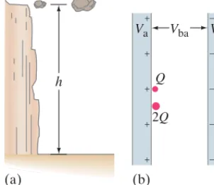
To better understand electric potential, let’s make a comparison to the gravi-tational case when a rock falls from the top of a cliff. The greater the height,h, of a cliff, the more potential energy the rock has at the top of the cliff relative to the bottom, and the more kinetic energy it will have when it reaches the bottom. The actual amount of kinetic energy it will acquire, and the amount of work it can do, depends both on the height of the cliff and the mass mof the rock. A large rock and a small rock can be at the same height h(Fig. 17–3a) and thus have the same “gravitational potential,” but the larger rock has the greater potential energy (it has more mass). The electrical case is similar (Fig. 17–3b): the potential energy change, or the work that can be done, depends both on the potential difference (corresponding to the height of the cliff) and on the charge (corresponding to mass), Eq. 17–3. But note a significant difference: electric charge comes in two types, and whereas gravitational mass is always

Sources of electrical energy such as batteries and electric generators are meant to maintain a potential difference. The actual amount of energy transformed by such a device depends on how much charge flows, as well as the potential dif-ference (Eq. 17–3). For example, consider an automobile headlight connected to a 12.0-V battery. The amount of energy transformed (into light and thermal energy) is proportional to how much charge flows, which in turn depends on how long the light is on. If over a given period of time 5.0 C of charge flows through

the light, the total energy transformed is If the headlight

is left on twice as long, 10.0 C of charge will flow and the energy transformed is Table 17–1 presents some typical voltages.

(10.0C)(12.0V) = 120J.

(5.0C)(12.0V) = 60J.

±.

–,

±

(=mgh)

+

+ + + +

−

− − − −

h

(a)

V_a V_ba V_b

(b)

Q

2Q

(5)

17–2

Relation between Electric Potential

and Electric Field

The effects of any charge distribution can be described either in terms of electric field or in terms of electric potential. Electric potential is often easier to use because it is a scalar, whereas electric field is a vector. There is an intimate connection between the potential and the field. Let us consider the case of a uniform electric field, such as that between the parallel plates of Fig. 17–1 whose difference of potential is The work done by the electric field to move a positive charge qfrom point a to point b is equal to the negative of the change in potential energy (Eq. 17–2b), so

We can also write the work done as the force times distance, where the force on qis so

wheredis the distance (parallel to the field lines) between points a and b. We

now set these two expressions for Wequal and find or

[uniform ] (17;4a)

If we solve for E, we find

[uniform ] (17;4b)

From Eq. 17–4b we see that the units for electric field can be written as volts

per meter , as well as newtons per coulomb ( , from ). These

are equivalent because The minus

sign in Eq. 17–4b tells us that EBpoints in the direction of decreasing potential V.

1N兾C = 1N⭈m兾C⭈m = 1J兾C⭈m = 1V兾m.

E = F兾q

N兾C

(V兾m)

EB

E = – V_dba.

EB

Vba = –Ed.

qV_ba = –qEd,

W = Fd = qEd,

F = qE,

W = –qAVb - VaB = –qVba.

Vba.

SECTION 17–2 Relation between Electric Potential and Electric Field

477

⫽ 50 V

d= 5.0 cm

E= ? + + + + + + + + + +

− − − − − − − − − −

V_ba

FIGURE 17–5 Example 17–3.

Electric field obtained from voltage. Two parallel plates are charged to produce a potential difference of 50 V. If the separation between the plates is 0.050 m, calculate the magnitude of the electric field in the space between the plates (Fig. 17–5).

APPROACH We apply Eq. 17–4b to obtain the magnitude of E, assumed uniform.

SOLUTION The magnitude of the electric field is

NOTE Equations 17–4 apply only for a uniform electric field. The general rela-tionship between EBand Vis more complicated.

E = Vba兾d = (50V兾0.050m) = 1000V兾m.

EXAMPLE 17;3

General Relation between

and

V

In a region where is not uniform, the connection between and Vtakes on a different form than Eqs. 17–4. In general, it is possible to show that the electric field in a given direction at any point in space is equal to the rate at which the electric potential decreases over distance in that direction. For example, the xcomponent

of the electric field is given by where is the change in

poten-tial over a very short distance

Breakdown Voltage

When very high voltages are present, air can become ionized due to the high electric fields. Any odd free electron can be accelerated to sufficient kinetic energy to knock electrons out of and molecules of the air. This breakdownof air occurs

when the electric field exceeds about When electrons recombine with

their molecules, light is emitted. Such breakdown of air is the source of lightning, the spark of a car’s spark plug, and even short sparks between your fingers and a doorknob after you walk across a synthetic rug or slide across a car seat (which can result in a significant transfer of charge to you).

3*106_V_兾_m.

N2

O2

¢x.

¢V

Ex = –¢V兾¢x,

EB EB

(6)

17–3

Equipotential Lines and Surfaces

The electric potential can be represented by drawing equipotential linesor, in three dimensions,equipotential surfaces. An equipotential surface is one on which all points are at the same potential. That is, the potential difference between any two points on the surface is zero, so no work is required to move a charge from one point on the surface to the other. An equipotential surface must be perpendicular to the electric field

at any point. If this were not so—that is, if there were a component of parallel to the surface—it would require work to move the charge along the surface against this component of and this would contradict the idea that it is an equipotential surface. The fact that the electric field lines and equipotential surfaces are mutually perpendicular helps us locate the equipotentials when the electric field lines are known. In a normal two-dimensional drawing, we show equipotential lines, which are the intersections of equipotential surfaces with the plane of the drawing. In Fig. 17–6, a few of the equipotential lines are drawn (dashed green lines) for the electric field (red lines) between two parallel plates at a potential difference of 20 V. The negative plate is arbitrarily chosen to be zero volts and the potential of each equipotential line is indicated. Note that points toward lower values of V. The equipotential lines for the case of two equal but oppositely charged particles are shown in Fig. 17–7 as green dashed lines. (This combination of equal and charges is called an “electric dipole,” as we saw in Section 16–8; see Fig. 16–32a.)

Unlike electric field lines, which start and end on electric charges, equipotential lines and surfaces are always continuous and never end, and so continue beyond the borders of Figs. 17–6 and 17–7. A useful analogy for equipotential lines is a topographic map: the contour lines are gravitational equipotential lines (Fig. 17–8). We saw in Section 16–9 that there can be no electric field within a conductor in the static case, for otherwise the free electrons would feel a force and would move. Indeed theentirevolume of a conductor must be entirely at the same potential in the static case. The surface of a conductor is thus an equipotential surface. (If it weren’t, the free electrons at the surface would move, because whenever there is a potential difference between two points, free charges will move.) This is fully consistent with our result in Section 16–9 that the electric field at the surface of a conductor must be perpendicular to the surface.

– ±

EB EB;

EB

– +

FIGURE 17–7 Equipotential lines (green, dashed) are always perpendicular to the electric field lines (solid red), shown here for two equal but oppositely charged particles (an “electric dipole”).

+ + + + + + + + + + + + + + + +

− − − − − − − − − − − − − − − − 20 V

15 V 10 V

0 V 5 V

EB

FIGURE 17–6 Equipotential lines (the green dashed lines) between two charged parallel plates are always perpendicular to the electric field (solid red lines).

FIGURE 17–8 A topographic map (here, a portion of the Sierra Nevada in California) shows continuous contour lines, each of which is at a fixed height above sea level. Here they are at 80-ft (25-m) intervals. If you walk along one contour line, you neither climb nor descend. If you cross lines, and especially if you climb perpendicular to the lines, you will be changing your gravitational potential (rapidly, if the lines are close together).

17–4

The Electron Volt, a Unit of Energy

The joule is a very large unit for dealing with energies of electrons, atoms, or molecules. For this purpose, the unit electron volt(eV) is used. One electron volt is defined as the energy acquired by a particle carrying a charge whose magnitude equals that on the electron as a result of moving through a potential difference of 1 V.

The charge on an electron has magnitude and the change in potential

energy equals qV. So 1 eV is equal to

An electron that accelerates through a potential difference of 1000 V will lose 1000 eV of potential energy and thus gain 1000 eV or 1 keV (kiloelectron volt) of kinetic energy.

1eV = 1.6022 * 10–19 _L _1.60 _* ₁₀–19_J.

A1.6022*10–19CB(1.00V)=1.6022*10–19J:

1.6022*10–19C,

(q = e)

(7)

On the other hand, if a particle with a charge equal to twice the magnitude of the

charge on the electron moves through a potential

differ-ence of 1000 V, its kinetic energy will increase by

Although the electron volt is handy for statingthe energies of molecules and elementary particles, it is nota proper SI unit. For calculations, electron volts should be converted to joules using the conversion factor just given. In Example 17–2, for

example, the electron acquired a kinetic energy of We can quote

this energy as 5000 eV but when determining

the speed of a particle in SI units, we must use the KEin joules (J). A= 8.0 * 10–16_J_兾_1.6 _* ₁₀–19_J_兾_eV_B_,

8.0 * 10–16_J.

2000eV = 2keV.

A= 2e = 3.2 * 10–19_C_B

SECTION 17–5 Electric Potential Due to Point Charges

479

C A U T I O N

for a point charge

Vr1

r, Er 1 r2

V

r

r V= kQ_r when Q > 0

V= kQ_r when Q < 0 0

V

0

(a)

(b)

FIGURE 17–9 Potential Vas a function of distance rfrom a single point charge Qwhen the charge is (a) positive, (b) negative.

EXERCISE B What is the kinetic energy of a ion released from rest and accelerated through a potential difference of 2.5 kV? (a) 2500 eV, (b) 500 eV, (c) 5000 eV, (d) 10,000 eV, (e) 250 eV.

He2±

17–5

Electric Potential Due to

Point Charges

The electric potential at a distance rfrom a single point charge Qcan be derived from the expression for its electric field (Eq. 16–4, ) using calculus. The potential in this case is usually taken to be zero at infinity ( , which means extremely, indefinitely, far away); this is also where the electric field

is zero. The result is

(17;5)

where We can think of Vhere

as representing the absolute potential at a distance rfrom the charge Q, where at or we can think of Vas the potential difference between rand infinity. (The symbol means infinitely far away.) Notice that the potential V

decreases with the first power of the distance, whereas the electric field (Eq. 16–4) decreases as the squareof the distance. The potential near a positive charge is large and positive, and it decreases toward zero at very large distances, Fig. 17–9a. The potential near a negative charge is negative and increases toward zero at large distances, Fig. 17–9b. Equation 17–5 is sometimes called the Coulomb potential

(it has its origin in Coulomb’s law). q

r = q;

V = 0

k = 8.99 * 109_N_⭈_m2_兾_C2 _L _9.0 _* ₁₀9_N_⭈_m2_兾_C2_.

= 1

4p⑀0

Q

r ,

csingle point charge_V ₌ _{0 at} _r _{= q} d

V = kQ_r

AE = kQ兾r2B

= q

E = kQ兾r2

Potential due to a positive or a negative charge. Deter-mine the potential at a point 0.50 m (a) from a point charge, (b) from a

point charge.

APPROACH The potential due to a point charge is given by Eq. 17–5,

SOLUTION (a) At a distance of 0.50 m from a positive charge, the potential is

(b) For the negative charge,

NOTE Potential can be positive or negative, and we always include a charge’s sign when we find electric potential.

V = A9.0 * 109_N_⭈_m2_兾_C2_B_¢–20 * 10–

6_C

0.50m ≤ = –3.6 * 10

5_V.

= A9.0 * 109_N_⭈_m2_兾_C2_B_¢20 * 10– 6_C

0.50m ≤ = 3.6 * 10

5_V.

V = kQ_r

20mC

V = kQ兾r.

–20mC

±20mC

EXAMPLE 17;4

P R O B L E M S O L V I N G

(8)

Work required to bring two positive charges close together. What minimum work must be done by an external force to bring a

charge from a great distance away (take ) to a point 0.500 m

from a charge

APPROACH To find the work we cannot simply multiply the force times distance because the force is proportional to and so is not constant. Instead we can set the change in potential energy equal to the (positive of the) work required of an

externalforce (Chapter 6, Eq. 6–7a), and Eq. 17–3: We get the potentials and using Eq. 17–5.

SOLUTION The external work required is equal to the change in potential energy:

where and The right-hand term within the parentheses is

zero so

NOTE We could not use Eqs. 17–4 here because they apply only to uniform fields. But we did use Eq. 17–3 because it is always valid.

Wext = A3.00 * 10–6CB

A8.99 * 109_N_⭈_m2_兾_C2_BA_2.00 _* ₁₀–5_C_B

(0.500m) = 1.08J.

(1兾q = 0)

ra = q.

rb = 0.500m

Wext = qAVb - VaB = q¢

kQ

rb

-kQ

ra ≤

, Va

Vb

Wext = ¢pe = qAVb - VaB.

1兾r2

Q = 20.0mC?

r = q

q = 3.00mC

EXAMPLE 17;5

C A U T I O N

We cannot use

if F is not constantW= Fd

C A U T I O N

Potential is a scalar and has no components

EXERCISE C What work is required to bring a charge originally a distance of 1.50 m from a charge Q = 20.0 mCuntil it is 0.50 m away?

q = 3.00 mC

To determine the electric field at points near a collection of two or more point charges requires adding up the electric fields due to each charge. Since the electric field is a vector, this can be time consuming or complicated. To find the electric potential at a point due to a collection of point charges is far easier, because the electric potential is a scalar, and hence you only need to add numbers (with appropriate signs) without concern for direction.

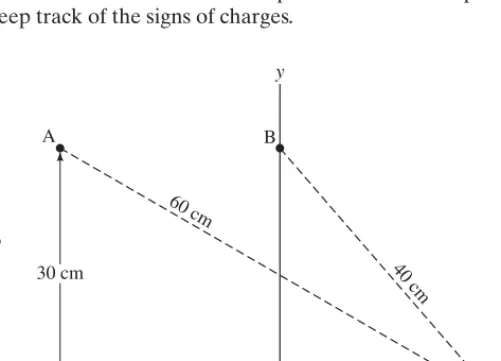
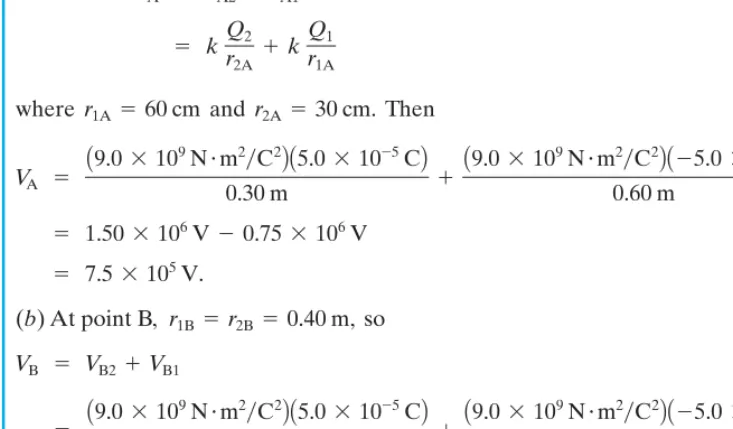
Potential above two charges. Calculate the electric poten-tial (a) at point A in Fig. 17–10 due to the two charges shown, and (b) at point B. [This is the same situation as Examples 16–9 and 16–10, Fig. 16–29, where we calculated the electric field at these points.]

APPROACH The total potential at point A (or at point B) is the algebraic sum of the potentials at that point due to each of the two charges and The potential due to each single charge is given by Eq. 17–5. We do not have to worry about directions because electric potential is a scalar quantity. But we do have to keep track of the signs of charges.

Q2.

Q1

EXAMPLE 17;6

A B

30 cm

26 cm 60 cm

40 cm

26 cm

Q₂= +50mC

x Q₁= −50mC y

(9)

SOLUTION (a) We add the potentials at point A due to each charge and and we use Eq. 17–5 for each:

where r1A = 60cm and Thenr2A = 30cm.

= kQ2

r2A + k

Q1

r1A

VA = VA2 + VA1

Q2,

Q1

SECTION 17–5 Electric Potential Due to Point Charges

481

+ –

+ +

(i)

(ii)

(iii)

FIGURE 17–11 Example 17–7. Simple summations like these can be performed for any number of point

charges.

Potential energies. Consider the three pairs of charges shown in Fig. 17–11. Call them and (a) Which set has a positive potential energy? (b) Which set has the most negative potential energy? (c) Which set requires the most work to separate the charges to infinity? Assume the charges all have the same magnitude.

RESPONSE The potential energy equals the work required to bring the two charges near each other, starting at a great distance Assume the left charge is already there. To bring a second charge close to the first from a great

distance away requires external work

whereris the final distance between them. Thus the potential energy of the two charges is

(a) Set (iii) has a positive potential energy because the charges have the same sign. (b) Both (i) and (ii) have opposite signs of charge and negative . Becauseris smaller in (i), the is most negative for (i). (c) Set (i) will require the most work for separation to infinity. The more negative the potential energy, the more work required to separate the charges and bring the up to zero (r = q),as in Fig. 17–9b.

pe pe

pe pe = kQ1_rQ2.

Wext = Q2V = k

Q1Q2

r

(q)

Q2

Q1

(±)

(q).

Q2.

Q1

CONCEPTUAL EXAMPLE 17;7

EXERCISE D Return to the Chapter-Opening Question, page 473, and answer it again now. Try to explain why you may have answered differently the first time.

(b) At point B, so

= 0V.

+ A9.0 * 10

9_N_⭈_m2_兾_C2_BA_–_5.0 _* ₁₀–5_C_B

0.40m

= A9.0 * 10

9_N_⭈_m2_兾_C2_BA_5.0 _* ₁₀–5_C_B

0.40m

VB = VB2 + VB1

r1B = r2B = 0.40m,

= 7.5 * 105_V.

= 1.50 * 106_V _- _0.75 _* ₁₀6_V

+ A9.0 * 10

9_N_⭈_m2_兾_C2_BA_–_5.0 _* ₁₀–5_C_B

0.60m

VA =

A9.0 * 109_N_⭈_m2_兾_C2_BA_5.0 _* ₁₀–5_C_B

0.30m

NOTE The two terms in the sum in (b) cancel for any point equidistant from

and Thus the potential will be zero everywhere on the plane

equidistant between the two opposite charges. This plane is an equipotential surface with V = 0.

Q2Ar1B = r2BB.

(10)

17–6

Potential Due to Electric Dipole;

Dipole Moment

Two equal point charges Q, of opposite sign, separated by a distance are called anelectric dipole. The electric field lines and equipotential surfaces for a dipole were shown in Fig. 17–7. Because electric dipoles occur often in physics, as well as in other disciplines such as molecular biology, it is useful to examine them more closely.

The electric potential at an arbitrary point P due to a dipole, Fig. 17–12, is the sum of the potentials due to each of the two charges:

whereris the distance from P to the positive charge and is the distance to the negative charge. This equation becomes simpler if we consider points P whose distance from the dipole is much larger than the separation of the two

charges—that is, for From Fig. 17–12 we see that since

we can neglect in the denominator as compared to r. Then we obtain

(17;6a)

We see that the potential decreases as the squareof the distance from the dipole, whereas for a single point charge the potential decreases with the first power of the distance (Eq. 17–5). It is not surprising that the potential should fall off faster for a dipole: when you are far from a dipole, the two equal but opposite charges appear so close together as to tend to neutralize each other.

The product in Eq. 17–6a is referred to as the dipole moment,p, of the dipole. Equation 17–6a in terms of the dipole moment is

(17;6b)

A dipole moment has units of coulomb-meters although for molecules a

smaller unit called a debyeis sometimes used:

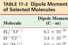
In many molecules, even though they are electrically neutral, the electrons spend more time in the vicinity of one atom than another, which results in a separation of charge. Such molecules have a dipole moment and are called polar molecules. We already saw that water (Fig. 16–4) is a polar molecule, and we have encoun-tered others in our discussion of molecular biology (Section 16–10). Table 17–2 gives the dipole moments for several molecules. The and signs indicate on which atoms these charges lie. The last two entries are a part of many organic molecules and play an important role in molecular biology.

– ±

1debye = 3.33 * 10–30_C_⭈_m.

(C⭈m),

[dipole; r W l]

V L kpcosu

r2 .

Ql

[dipole; r W l]

V L kQlcosu

r2 .

¢r

r W ¢r = lcosu,

¢r = lcosu;

r W l.

r + ¢r

V = kQ_r + k(–Q)_r _{+ ¢}

r = kQa

1

r

-1

r + ¢rb = kQ

¢r

r(r + ¢r),

l,

*

P H Y S I C S A P P L I E D

Dipoles in molecular biology

Uses of capacitors

TABLE 17–2 Dipole Moments of Selected Molecules

Dipole Moment Molecule

‡

‡_{These last two groups often appear on} larger molecules; hence the value for the dipole moment will vary somewhat, depending on the rest of the molecule.

L8.0 * 10–30 »C(±)“O(–)

L3.0 * 10–30 »N(–)¬H(±)

5.0 * 10–30 N(–)H3(±)

3.4 * 10–30 H(±)Cl(–)

6.1 * 10–30 H2(±)O(–)

(Cⴢm)

r r

l

P

u

Δr

−Q +Q

FIGURE 17–12 Electric dipole. Calculation of potential Vat point P.

17–7

Capacitance

(11)

A simple capacitor consists of a pair of parallel plates of area Aseparated by a small distance d(Fig. 17–13a). Often the two plates are rolled into the form of a cylinder with paper or other insulator separating the plates, Fig. 17–13b; Fig. 17–13c is a photo of some actual capacitors used for various applications. In circuit diagrams, the symbol

or [capacitor symbol]

represents a capacitor. A battery, which is a source of voltage, is indicated by the symbol

[battery symbol]

with unequal arms.

If a voltage is applied across a capacitor by connecting the capacitor to a bat-tery with conducting wires as in Fig. 17–14, charge flows from the battery to each of the two plates: one plate acquires a negative charge, the other an equal amount of positive charge. Each battery terminal and the plate of the capacitor connected to it are at the same potential; hence the full battery voltage appears across the capacitor. For a given capacitor, it is found that the amount of charge Qacquired by each plate is proportional to the magnitude of the potential difference Vbetween the plates:

(17;7)

The constant of proportionality, C, in Eq. 17–7 is called the capacitance of the capacitor. The unit of capacitance is coulombs per volt, and this unit is called a farad (F). Common capacitors have capacitance in the range of 1 pF

to The relation, Eq. 17–7,

was first suggested by Volta in the late eighteenth century.

In Eq. 17–7 and from now on, we will use simply V(in italics) to represent a potential difference, such as that produced by a battery, rather than or

as previously.

Also, be sure not to confuse italiclettersVandCwhich stand for voltage and capacitance, with non-italic V and C which stand for the units volts and coulombs. The capacitance Cdoes not in general depend on QorV. Its value depends only on the size, shape, and relative position of the two conductors, and also on the material that separates them. For a parallel-plate capacitor whose plates have area A

and are separated by a distance dof air (Fig. 17–13a), the capacitance is given by

[parallel-plate capacitor] (17;8)

We see that Cdepends only on geometric factors, Aandd, and not on Q orV. We derive this useful relation in the optional subsection at the end of this Section. The constant is the permittivity of free space, which, as we saw in Chapter 16, has the value 8.85 * 10–12C2兾N⭈m2.

⑀0

C = ⑀0A

d.

Vb - Va,

Vba, ¢V,

Amicrofarad = 10–6_F_B_.

103_m_F

Apicofarad = 10–12_F_B

Q = CV.

ⴙ ⴚ

SECTION 17–7 Capacitance

483

C A U T I O N

difference from here on

V = potential

d

(a) (b) (c)

Insulator

A

FIGURE 17–13

Capacitors: diagrams of (a) parallel plate, (b) cylindrical (rolled up parallel plate). (c) Photo of some real capacitors.

EXERCISE E Graphs for charge versus voltage are shown in Fig. 17–15 for three capac-itors, A, B, and C. Which has the greatest capacitance?

12 V

ⴙQⴚQ

C

V

ⴙ ⴚ ⴙ ⴚ

(a) (b)

− − − − − − + + + + + +

FIGURE 17–14 (a) Parallel-plate capacitor connected to a battery. (b) Same circuit shown using symbols.

A

B

C Q

(12)

Capacitor calculations. (a) Calculate the capacitance of a

parallel-plate capacitor whose plates are and are separated by a

1.0-mm air gap. (b) What is the charge on each plate if a 12-V battery is connected across the two plates? (c) What is the electric field between the plates? (d) Esti-mate the area of the plates needed to achieve a capacitance of 1 F, assuming the

air gap dis 100 times smaller, or 10 microns (1 micron .

APPROACH The capacitance is found by using Eq. 17–8, The charge on each plate is obtained from the definition of capacitance, Eq. 17–7, The electric field is uniform, so we can use Eq. 17–4b for the magnitude

In (d) we use Eq. 17–8 again.

SOLUTION (a) The area .

The capacitance Cis then

(b) The charge on each plate is

(c) From Eq. 17–4b for a uniform electric field, the magnitude of Eis

(d) We solve for Ain Eq. 17–8 and substitute and to find that we need plates with an area

NOTE This is the area of a square or 1 km on a side. That is inconven-iently large. Large-capacitance capacitors will not be simple parallel plates.

103_m

A = Cd_⑀

0 L

(1F)A1.0 * 10–5mB

A9 * 10–12_C2_兾_N_⭈_m2_B L 10 6_m2_.

d = 1.0 * 10–5_m

C = 1.0F

E = V_d = 12V

1.0 * 10–3_m = 1.2 * 10

4_V_兾_m.

= A53 * 10–12_F_B₍₁₂_V₎ ₌ _6.4 _* ₁₀–10_C.

Q = CV

= A8.85 * 10–12_C2_兾_N_⭈_m2_B6.0 * 10– 3_m2

1.0 * 10–3_m = 53pF.

C = ⑀0

A d

A = A20 * 10–2_m_BA_3.0 _* ₁₀–2_m_B ₌ _6.0 _* ₁₀–3_m2

E = V兾d.

Q = CV.

C = ⑀0A兾d.

= 1mm = 10–6_m₎

20cm * 3.0cm

EXAMPLE 17;8

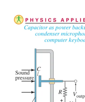
Capacitor as power backup; condenser microphone; computer keyboard

Not long ago, a capacitance greater than a few mF was unusual. Today capacitors are available that are 1 or 2 F, yet they are just a few cm on a side. Such capacitors are used as power backups, for example, in computer memory and electronics where the time and date can be maintained through tiny charge flow. [Capacitors are superior to rechargable batteries for this purpose because they can be recharged more than times with no degradation.] Such high-capacitance capacitors can be made of activated carbonwhich has very high porosity, so that the surface area is very large; one-tenth of a gram of activated carbon can have a surface area of Furthermore, the equal and opposite charges exist in an electric “double layer” about thick. Thus, the capacitance of 0.1 g of activated carbon, whose internal area can be is equivalent to a parallel-plate capacitor with

The proportionality, in Eq. 17–8, is valid also for a parallel-plate capacitor that is rolled up into a spiral cylinder, as in Fig. 17–13b. However, the constant factor, must be replaced if an insulator such as paper separates the plates, as is usual, as discussed in the next Section.

One type of microphone is a condenser, or capacitor,microphone, diagrammed in Fig. 17–16. The changing air pressure in a sound wave causes one plate of the capacitorCto move back and forth. The voltage across the capacitor changes at the same frequency as the sound wave.

Some computer keyboards operate by capacitance. As shown in Fig. 17–17, each key is connected to the upper plate of a capacitor. The upper plate moves down when the key is pressed, reducing the spacing between the capacitor plates, and increasing the capacitance (Eq. 17–8: smaller d, larger C). The change

in capacitance results in an electric signal that is detected by an electronic circuit.

⑀0,

C r A兾d

C L ⑀0A兾d = A8.85 * 10–12C2兾N⭈m2BA102m2B兾A10–9mB L 1F.

102_m2_,

10–9_m

100m2_.

105

Key

Insulator (ﬂexible) Movable plate

Fixed plate Capacitor FIGURE 17–17 Key on a computer keyboard. Pressing the key reduces the plate spacing, increasing the capacitance. FIGURE 17–16 Diagram of a condenser microphone.

Sound pressure

R

V + –

V_output C

(13)

SECTION 17–8

485

TABLE 17–3

Dielectric Constants (at 20°C)

Dielectric Dielectric constant strength Material K

Vacuum 1.0000 Air (1 atm) 1.0006 Paraffin 2.2 Polystyrene 2.6 Vinyl (plastic) 2–4

Paper 3.7 Quartz 4.3 Oil 4 Glass, Pyrex 5

Rubber,

neoprene 6.7 Porcelain 6–8

Mica 7 Water (liquid) 80

Strontium

titanate 300 8 * 106

150 * 106 5 * 106 12 * 106 14 * 106 12 * 106 8 * 106 15 * 106 50 * 106 24 * 106 10 * 106 3 * 106 (V

Ⲑ

m) FIGURE 17–18 A cylindrical capacitor, unrolled from its case to show the dielectric between the plates. See also Fig. 17–13b.

Derivation of Capacitance for Parallel-Plate Capacitor

Equation 17–8 can be derived using the result from Section 16–12 on Gauss’s law, namely that the electric field between two parallel plates is given by Eq. 16–10:

We combine this with Eq. 17–4a, using magnitudes, to obtain

Then, from Eq. 17–7, the definition of capacitance,

which is Eq. 17–8.

17–8

Dielectrics

In most capacitors there is an insulating sheet of material, such as paper or plastic, called a dielectricbetween the plates (Fig. 17–18). This serves several purposes. First, dielectrics break down (allowing electric charge to flow) less readily than air, so higher voltages can be applied without charge passing across the gap. Further-more, a dielectric allows the plates to be placed closer together without touching, thus allowing an increased capacitance because dis smaller in Eq. 17–8. Thirdly, it is found experimentally that if the dielectric fills the space between the two con-ductors, it increases the capacitance by a factor K, known as the dielectric constant. Thus, for a parallel-plate capacitor,

(17;9)

This can be written

where is called the permittivityof the material.

The values of the dielectric constant for various materials are given in Table 17–3. Also shown in Table 17–3 is the dielectric strength, the maximum electric field before breakdown (charge flow) occurs.

⑀ = K⑀0

C = ⑀ A

d,

C = K⑀0A

d.

C = Q_V = Q

AQ兾A⑀0Bd

= ⑀0

A d

V = ¢ Q

A⑀0

≤d.

V = Ed,

E = Q_⑀兾A

0

.

*

Inserting a dielectric at constant V. An air-filled capacitor consisting of two parallel plates separated by a distance dis connected to a battery of constant voltage Vand acquires a charge Q. While it is still connected to the battery, a slab of dielectric material with is inserted between the plates of the capacitor. Will Qincrease, decrease, or stay the same?

RESPONSE Since the capacitor remains connected to the battery, the voltage stays constant and equal to the battery voltage V. The capacitance Cincreases when the dielectric material is inserted because Kin Eq. 17–9 has increased. From the relation if Vstays constant, but Cincreases,Qmust increase as well. As the dielectric is inserted, more charge will be pulled from the battery and deposited onto the plates of the capacitor as its capacitance increases.

Q = CV,

K = 3

CONCEPTUAL EXAMPLE 17;9

EXERCISE F If the dielectric in Example 17–9 fills the space between the plates, by what factor does (a) the capacitance change, (b) the charge on each plate change?

Inserting a dielectric into an isolated capacitor. Suppose the air-filled capacitor of Example 17–9 is charged (to Q) and then disconnected from the battery. Next a dielectric is inserted between the plates. Will Q,C, or Vchange?

RESPONSE The charge Qremains the same—the capacitor is isolated, so there is nowhere for the charge to go. The capacitance increases as a result of inserting the dielectric (Eq. 17–9). The voltage across the capacitor also changes—it

decreases because, by Eq. 17–7, so if Q stays constant andCincreases (it is in the denominator), then Vdecreases.

V = Q兾C;

Q = CV,

(14)

Camera flash

(a)

ⴙ ⴚ

ⴙQ ⴚQ

(b)

ⴙ ⴚ

ⴙ _ⴚⴙⴚⴙ ⴚ

ⴚⴙ ⴚⴙ ⴚⴙ ⴚⴙ ⴚⴙ

ⴚⴙ ⴚⴙ ⴚⴙ ⴚⴙ ⴚⴙ ⴚⴙ ⴚⴙ

ⴚ ⴙ

ⴙ ⴚ

(c)

E₀ E₀

FIGURE 17–19 Molecular view of the effects of a dielectric.

Molecular Description of Dielectrics

Let us examine, from the molecular point of view, why the capacitance of a capacitor should be larger when a dielectric is between the plates. A capacitor whose plates are separated by an air gap has a charge on one plate and on the other (Fig. 17–19a). Assume it is isolated (not connected to a battery) so charge cannot flow to or from the plates. The potential difference between the plates, is given by Eq. 17–7:

where the subscripts refer to air between the plates. Now we insert a dielectric between the plates (Fig. 17–19b). Because of the electric field between the capac-itor plates, the dielectric molecules will tend to become oriented as shown in Fig. 17–19b. If the dielectric molecules are polar, the positive end is attracted to the negative plate and vice versa. Even if the dielectric molecules are not polar, electrons within them will tend to move slightly toward the positive capacitor plate, so the effect is the same. The net effect of the aligned dipoles is a net nega-tive charge on the outer edge of the dielectric facing the posinega-tive plate, and a net positive charge on the opposite side, as shown in Fig. 17–19c.

Some of the electric field lines, then, do not pass through the dielectric but instead end on charges induced on the surface as shown in Fig. 17–19c. Hence the electric field within the dielectric is less than in air. That is, the electric field in the space between the capacitor plates, assumed filled by the dielectric, has been reduced by some factor K. The voltage across the capacitor is reduced by the same factor Kbecause (Eq. 17–4) and hence, by Eq. 17–7,

the capacitance Cmust increase by that same factor Kto keep Qconstant.

17–9

Storage of Electric Energy

A charged capacitor stores electric energy by The

energy stored in a capacitor will be equal to the work done to charge it. The net effect of charging a capacitor is to remove charge from one plate and add it to the other plate. This is what a battery does when it is connected to a capacitor. A capacitor does not become charged instantly. It takes some time, often very little (Section 19–6). Initially, when the capacitor is uncharged, no work is required to move the first bit of charge over. As more charge is transferred, work is needed to move charge against the increasing voltage V. The work needed to add a small amount of charge when a potential difference V is across the plates, is The total work needed to move total charge Q is equivalent to moving all the charge Q across a voltage equal to the average voltage during the process. (This is just like calculating the work done to compress a spring,

Section 6–4, page 148.) The average voltage is where is the

final voltage; so the work to move the total charge Qfrom one plate to the other is

Thus we can say that the electric potential energy,PE, stored in a capacitor is

whereVis the potential difference between the plates (we dropped the subscript),

andQis the charge on each plate. Since we can also write

(17;10)

Energy stored in a capacitor. A camera flash unit (Fig. 17–20) stores energy in a capacitor at 330 V. (a) How much electric energy can be stored? (b) What is the power output if nearly all this energy is released in 1.0 ms?

APPROACH We use Eq. 17–10 in the form because we are given

CandV.

pe ₌ 1 2CV2

660-mF

EXAMPLE 17;11

pe = 1

2QV =

1

2CV

2 ₌ 1

2

Q2

C .

Q = CV,

pe = energy = 12QV,

W = QVf

2.

Vf AVf - 0B兾2 = Vf兾2,

¢W = V¢q.

¢q,

separating + and - charges.

Q = CV,

V = Ed

Q = C0V0,

V0,

–Q

±Q C0

(15)

SECTION 17–9 Storage of Electric Energy

487

FIGURE 17–20 A camera flash unit. The capacitor is the black cylinder.

660-mF

SOLUTION (a) The energy stored is

(b) If this energy is released in of a second the

power output is P = pe兾t = (36J)兾A1.0 * 10–3_sA_B=₌ _36,000_W.

1.0ms = 1.0 * 10–3_s_B_,

1 1000 pe = 1

2CV2 =

1

2A660 * 10–6FB(330V)2 = 36J.

EXERCISE G A capacitor stores 0.50 J of energy at 9.0 V. What is its capacitance?

Capacitor plate separation increased.

A parallel-plate capacitor carries charge Qand is then disconnected from a battery. The two plates are initially separated by a distance d. Suppose the plates are pulled apart until the separation is 2d. How has the energy stored in this capacitor changed?

RESPONSE If we increase the plate separation d, we decrease the capacitance

according to Eq. 17–8, by a factor of 2. The charge Q hasn’t

changed. So according to Eq. 17–10, where we choose the form

because we know Qis the same and Chas been halved, the reduced Cmeans thePEstored increases by a factor of 2.

NOTE We can see why the energy stored increases from a physical point of view: the two plates are charged equal and opposite, so they attract each other. If we pull them apart, we must do work, so we raise the potential energy.

pe = 1 2Q2兾C

C = ⑀0A兾d,

CONCEPTUAL EXAMPLE 17;12

It is useful to think of the energy stored in a capacitor as being stored in the electric field between the plates. As an example let us calculate the energy stored in a parallel-plate capacitor in terms of the electric field.

We have seen that the electric field between two close parallel plates is nearly uniform and its magnitude is related to the potential difference by

(Eq. 17–4), where dis the separation. Also, Eq. 17–8 tells us for a parallel-plate capacitor. Thus

The quantity Adis the volume between the plates in which the electric field E

exists. If we divide both sides of this equation by the volume, we obtain an expression for the energy per unit volume or energy density:

(17;11)

The electric energy stored per unitvolume in any region of space is proportional to the square of the electric fieldin that region. We derived Eq. 17–11 for the special case of a parallel-plate capacitor. But it can be shown to be true for any region of space where there is an electric field. Indeed, we will use this result when we dis-cuss electromagnetic radiation (Chapter 22).

Health Effects

The energy stored in a large capacitance can give you a burn or a shock. One reason you are warned not to touch a circuit, or open an electronic device, is because capacitors may still be carrying charge even if the external power is turned off. On the other hand, the basis of a heart defibrillatoris a capacitor charged to a high voltage. A heart attack can be characterized by fast irregular beating of the heart, known as ventricular(orcardiac)fibrillation. The heart then does not pump blood to the rest of the body properly, and if the interruption lasts for long, death results. A sudden, brief jolt of charge through the heart from a defibrillator can cause complete heart stoppage, sometimes followed by a resumption of normal beating. The defibrillator capacitor is charged to a high voltage, typically a few thousand volts, and is allowed to discharge very rapidly through the heart via a pair of wide contacts known as “pads” or “paddles” that spread out the current over the chest (Fig. 17–21).

energy density = pe

volume =

1 2⑀0E2.

= 1

2⑀0E2Ad. pe = 1₂CV2 ₌ 1

2¢

⑀0A

d ≤AE2d2B

C = ⑀0A兾d

V = Ed

EB

Shocks, burns, defibrillators

(16)

FIGURE 17–22 Two kinds of signal voltage: (a) sinusoidal, (b) a pulse, both analog. Many other shapes are possible.

FIGURE 17–24 The red analog sine wave, which is at a 100-Hz frequency (1 wavelength is done in 0.010 s), has been converted to a 2-bit (4 level) digital signal (blue).

time,t V

0

(a)

time,t V

0

(b)

TABLE 17–4

Binary to Decimal

Binary† _Decimal number number

00000000 0

00000001 1

00000010 2

00000011 3

00000100 4

00000111 7

00001000 8

00100101 37

11111111 255

†_{Note that we start counting from right} to left: the 1’s digit is on the far right, then the 2’s, the 4’s, the 8’s, the 16’s, the 32’s, the 64’s, and the 128’s.

0 s

0.010 s 10

01

00

Bit levels 0V

6V

11

t

A “1” is a positive voltage such as , whereas a “0” is . The brightness signal, for example, that goes to each of the millions of tiny picture elements or “subpixels” of a TV or computer screen (Fig. 17–31, Section 17–11), is contained in a byte. One byte is 8 bits, which means

each byte of 8 bits allows possibilities

(that is, 0 to 255) or 256 shades for each of 3 colors: red, green, blue. The full

color of each pixel (the three subpixel colors) has possibilities.

Digital television signals, which we discuss in the next Section, are transmitted

at about Megabits per second. So pass a given point

per second, or one bit every 53 nanoseconds. We could write this in terms of bytes as 2.4 MB s, where for bytes we use capital B.

When an analog signal, such as the pure sine wave of Fig. 17–22a, is converted to digital (analog-to-digital converter, ADC), the digital signal may look like the blue squared-off curve of Fig. 17–24. The digital signal has a limited number of discrete values. The difference between the original continuous analog signal and its digital approximation is called the quantization errororquantization loss. To min-imize that loss, there are two important factors: (i) the resolutionorbit depth, which is the number of bits or values for the voltage of each sample ( measurement); (ii) the sampling rate, which is the number of times per second the original analog voltage is measured (“sampled”).

Consider a digital approximation for a 100-Hz sine wave: Figure 17–24 shows (i) a 0 to 6-V, 2-bit depth, measuring only 4 possible voltages (00, 01, 10, 11, or 0, 1, 2, 3 in decimal), and (ii) a sampling rate of (9 samples in one cycle or

wavelength 100 cycles ) which is 900 samples s or 900 Hz. This is very

poor quality. For high quality reproduction, a greater bit depth and higher sampling

兾兾s=100Hz

)*(

=

兾

19 * 106_bits

19Mb兾s = 19

(256)3 ₌ ₁₇ _* ₁₀6

28 ₌ ₂₅₆

0V

±5V

17–10

Digital; Binary Numbers;

Signal Voltage

Batteries and a wall plug are meant to provide a constant supply voltageas power to operate a flashlight, an electric heater, and other electric and electronic devices. Asignal voltage, on the other hand, is a voltage intended to affect something else. A signal voltage varies in time and can also be very brief. For example, a sound such as a pure tone, which may be sinusoidal as we discussed in Chapters 11 and 12 (see Figs. 11–24 and 12–14), will produce an output voltage from a high quality microphone that is also sinusoidal. That signal voltage is amplified and reaches a loudspeaker, making it produce the sound we hear. Signal voltages (see Fig. 17–22) are sometimes a simple pulse (as in Figs. 11–23 and 11–33), and often act to change some aspect of an electronic device.

Signal voltages are sent to cell phones (“I’ve got signal”), to computers from the Internet, or to TV sets with the information on the picture and sound. Not long ago, signal voltages were analog—the voltage varied continuously, as in Fig. 17–22. Today, television and computer signals are digitaland use a binary number system to represent a numerical value. In a normal number, such as 609, there are

tenchoices for each digit—from 0 to 9—and normal numbers are called decimal

(Latin for ten). In a binarynumber, each digit or bithas only twopossibilities, 0 or 1 (sometimes referred to as “off” or “on”). In binary, 0001 means “one,”

0010 means 2, 0011 means 3, and 1101 means in decimal.

See Table 17–4, and note that counting starts from the right, just as in regular decimal (the “ones” digit is last, on the far right, then to the left is the “tens” and then “hundreds”: for 609, the “ones” are 9, the “hundreds” are 6). Any value can be represented by a voltage pattern something like that shown in Fig. 17–23.

8 + 4 + 0 + 1 = 13

FIGURE 17–23 A traveling digital signal: voltage vs. position xor time . If standing alone, this sequence would represent 10011001 or 153

0 + 16 + 8 + 0+ 0 + 1).

(⫽ 128 + 0 +

t

t orx

5 V

64’s

128’s 32’s 16’s 8’s 4’s 2’s 1’s

(17)

SECTION 17–10

489

For audio CDs, the sampling rate is 44.1 kHz (44,100 samplings every second) and 16-bit resolution, meaning each sampled voltage can have

different voltage levels between, say, 0 and 5 volts. See Fig. 17–25 for details.

Audio recording today typically uses 96 kHz and 24-bit ( voltage

levels) to give a better approximation of the original analog signal (on super-CDs or solid-state memory), but must be transferred down to 44.1 kHz and 16-bit to produce ordinary CDs. (DVDs can use 192 kHz sampling rate for sound.) But iPods and MP3 players have lower sampling rates and much less detail, which many listeners can notice.

224 _L ₁₇ _* ₁₀6

28_*₂8₌₂16_L _65,000

FIGURE 17–25 The sine wave shown could represent the analog electric signal from a microphone due to a pure 2000-Hz tone. (See Chapters 11 and 12.) The analog-to-digital electronics samplesthe signal—that is, measures and records the signal’s voltage at intervals, many times per second. Each dot on the curve represents the voltage measured (sampled) at that point. The sampling rate in this diagram is 44,100 each second, or 44.1 kHz,

like a CD. That is, a sample is taken every .

In 0.50 ms, as shown here, 22 samples (black dots) are taken. This is an alternate way to represent sampling compared to Fig. 17-24, and shows that we cannot see any changes that might happen between the samplings (dots).

(1 s)兾44,100 = 0.000023 s = 0.023 ms t

V

0

0.25 ms 0.50 ms

Voltage

Figure 17–25 gives some details about a pure 2000-Hz sound sampled at 44.1 kHz. Normal musical sounds are a complex summation of many such sine waves of different frequencies and amplitudes. A simple summation was shown in Fig. 12–14. Another example is shown in Fig. 17–26, where we can see that the fine details may be missed by a digital conversion. Look at Fig. 17–25: if that were 20,000 Hz (highest frequency of human hearing), it would be sampled only about two times per wavelength. Both those samples might be zero volts—obviously missing the entire waveform. Over many wavelengths, it might eventually reproduce the waveform somewhat well. But many sounds only last milliseconds, like the initial attack of a piano note or plucked guitar string. Many audiophiles hear the difference between an original vinyl record and its subsequent release as a CD at 44.1 kHz.

Digital audio signals must be converted back to analog (digital-to-analog converter, DAC) before being sent to a loudspeaker or headset. Even in a TV, the digital signals are converted to analog voltages before addressing the pixels (next Section), although the picture itself might be said to be digital since it is made up of separate pixels.

Digital photographs are made up of millions of “pixels” to produce a sharp image that is not “pixelated” or blurry. Also important (and complicated) are the number of bits provided for colors, plus the ability of the sensors (Chapter 25) to sustain a wide range of brightnesses under dim and bright light conditions.

Digital data has some real advantages: for one, it can be compressed, in the sense that repeated information can be reduced so that less memory space is required—fewer bits and bytes. For example, adjacent “pixels” on a photograph that includes a blue sky may be essentially identical. If 200 almost identical pixels can be coded as identical, that takes up less memory (or “size”) than to specify all the 200 pixels individually. Compression schemes, like jpegfor photos, lose some information and may be noticeable. In audio, MP3 players use one-tenth the space that a CD does, but many listeners don’t notice. Compression is one reason that more data or “information” can be transmitted digitally for a given bandwidth. [Bandwidth is the fixed range of frequencies allotted to each radio or TV station or Internet connection, and limits the number of bits transmitted per second.]

In audio, many listeners claim that digital does not match analog in full sound quality. And what about movies? Will digital ever match Technicolor?

Noise

Digital information transmission has another advantage: any distortion or unwanted (external) electrical signal that intrudes from outside, broadly called noise, can badly corrupt an analog signal: Fig. 17–27a shows a time-varying analog signal, and Fig. 17–27b shows nasty outside noise interfering with it. But a digital signal is still readable unless the noise is very large, on the order of half the bit signal itself (Figs. 17–27c and d).

*

t V

0

FIGURE 17–26 This type of complex signal is much more normal than the pure sine wave of Fig. 17–25.

Sampling may not catch all the details, especially because the waveform is changing very fast in time.

(a) Analog signal

(b) Analog signal plus noise

(c) Digital signal

(d) Digital signal plus noise FIGURE 17–27 (a) Original analog signal and (b) the same signal dirtied up by outside signals ( noise). (c) A digital signal is still readable (d) without error if the noise is not too great.

(18)

17–11

TV and Computer Monitors:

CRTs, Flat Screens

The first television receivers used a cathode ray tube (CRT), and as recently as 2008 they accounted for half of all new TV sales. Two years later it was tough to find a new CRT set to buy. Even though new TV sets are flat screen plasma or

liquid crystal displays(LCD), an understanding of how a CRT works is useful.

CRT

The operation of a CRT depends on thermionic emission, discovered by Thomas Edison (1847–1931). Consider a voltage applied to two small electrodes inside an evacuated glass “tube” as shown in Fig. 17–28: the cathodeis negative, and the

anodeis positive. If the cathode is heated (usually by an electric current) so that it becomes hot and glowing, it is found that negative charges leave the cathode and flow to the positive anode. These negative charges are now called electrons, but originally they were called cathode rays because they seemed to come from the cathode (more detail in Section 27–1 on the discovery of the electron).

Figure 17–29 is a simplified sketch of a CRT which is contained in an evacuated glass tube. A beam of electrons, emitted by the heated cathode, is accelerated by the high-voltage anode and passes through a small hole in that anode. The inside of the tube face on the right (the screen) is coated with a fluorescent material that glows at the spot where the electrons hit. Voltage applied across the horizontal and vertical deflection plates, Fig. 17–29, can be varied to deflect the electron beam to different spots on the screen.

*

CRT

Anode Cathode

Batteryⴚ ⴙ

ⴚ ⴙ

FIGURE 17–28 If the cathode inside the evacuated glass tube is heated to glowing (by an electric current, not shown), negatively charged “cathode rays” ( electrons) are “boiled off” and flow across to the anode to which they are attracted.

(±),

=

Heater current

Cathode Anode

Horizontal deﬂection plates

Bright spot on screen where electrons hit Grid

Vertical deﬂection plates

Path of electrons

Fluorescent screen

FIGURE 17–29 A cathode-ray tube. Magnetic deflection coils are commonly used in place of the electric deflection