Vol. 11, No. 2, 2016, 1-6
ISSN: 2279-087X (P), 2279-0888(online) Published on 2 March 2016
www.researchmathsci.org
1
Annals of
Numerical Solution to Euler–Cauchy Equation with
Neumann Boundary Conditions Using B-Spline
Collocation Method
Y. Rajashekhar Reddy Department of Mathematics, JNTUHCollege of Engineering Jagitial, Nachupally (Kondagattu) Karimnagar, Telangana State, PIN-505501, India
Email: [email protected]
Received 29 January 2016; accepted 18 February 2016
Abstract. Third degree B-spline basis functions are used as basis functions in collocation method to approximate the solution of second order Euler–Cauchy equations with Neumann boundary conditions. Recursive form of B-spline function is used as basis in this present method. This method is demonstrated by considering Euler–Cauchy equations with Neumann boundary condition problems. The results are compared with exact solutions to find its efficiency and consistency. The easiness of the method reduces the complexity and time consuming when compared with other existed methods.
Keywords: B-splines, collocation, Euler–Cauchy equations, Neumann boundary conditions
AMS Mathematics Subject Classification (2010): 34A45 1. Introduction
In this paper Euler- Cauchy’s type of equation of the form
b x a U a dx
U d x a dx
U d x a dx
U d x
a n
n n n n
n n n
n
n + + + + = ≤ ≤
− −
− − −
−
− ... 0,
1 2
2 2 2 1 1 1 1
0 (1)
, where ‘U’ is a function in ‘x’, is considered with the boundary conditions
n
n b k
U k b U k b U k b U k b
U( )= 1, '( )= 2, ''( )= 3, '''( )= 4 ... −1( )= .
The above form of Euler-Cauchy homogeneous linear differential equations are solved by modifying into linear differential equation with constant coefficients. In this process, the solution is obtained to the modified differential equation and processes are involved in finding the solutions for such type of Euler –Cauchy homogeneous linear differential equations.
2
calculations such as integrations, transforming the given equation into linear equation with constant coefficients and suitable substitutions etc.
Let = ∑−
− =
1
2 ,
) ( )
( m
i i i p
h
x N C x
U (2)
where
C
i’s are constants to be determined andN
i,p(
x
)
are B-spline basis functions, be the approximate global solution to the exact solutionU
(x
)
of the considered nth order Euler- Cauchy’s differential equation (1).2. B-splines
In this section, definition and properties of B-spline basis functions [1-3] are given in detail. A zero degree and higher degree B-spline basis functions are defined at
x
i
recursively over the knot vector spaceX ={x1,x2,x3... xm−1,xm} as
i
)
if
p
=
0
1
)
(
,x
=
N
i pif
x
∈
(
x
i,
x
i+i)
0
)
(
,x
=
N
i pif
x
∉
(
x
i,
x
i+i)
ii
)
if
p
≥
1
)
(
)
(
)
(
1, 11 1
1 1
,
,
N
x
x
x
x
x
x
N
x
x
x
x
x
N
i pi p i
p i p
i i p i
i p
i + −
+ + +
+ + −
+
−
−
+
−
−
=
where p is the degree of the B-spline basis function and
x
is the parameter belongs to X. When evaluating these functions, ratios of the form 0/0 are defined as zero.3. B-spline collocation method
Collocation method is widely used in approximation theory particularly to solve differential equations .In collocation method, the assumed approximate solution is made it exact at some nodal points by equating residue zero at that particular node. B-spline basis functions are used as the basis in B-spline collocation method whereas the base functions which are used in normal collocation method are the polynomials vanishes at the boundary values. Residue which is obtained by substituting equation (2) in equation (1) is made equal to zero at nodes in the given domain to determine unknowns in (2). Let
[ b
a
,
]
be the domain of the governing differential equation and is partitioned as} ,
...
{a x0,x1,x2 x 1 x b
X = = m− m =
with equal length
m
a
b
h
=
−
ofm
-subdomains. The
x '
i
s
are known as nodes, the nodes are treated as knots in collocation B-spline method where B-B-spline basis functions are defined and these nodes are used to make the residue equal to zero to determine unknownsC '
i
s
in (2), two extra knot vectors are taken into consideration beside the domain of problem both side when evaluating the second degree B-spline basis functions at the nodes.Using B-Spline Collocation Method 3 0 . . . 1 2 2 2 2 1 1 1 1
0 + + − + + − =
− − − − − h n n h n n n h n n n h n
n a U
dx U d x a dx U d x a dx U d x a i.e. 0 ) ( . . . ) ( ) ( 1 2 , 1 1 2 , 1 1 1 1 2 ,
0 ∑ + ∑ + + ∑ =
− − = − − − = − − − − = m i p i i n m i p i n i n m i p i n i
n C N x a x C N x a C N x
x
a (3)
Equation (3) which is evaluated at
x '
i
s
,i=0, 1, 2,....m-1 gives the system of (m-2) × (m+1) equations in which (m+1) arbitrary constants are involved. Particularly for third degree i.e m=3, three more equations are needed to have (m+1) × (m+1) square matrix which helps to determine the (m+ 1) arbitrary constants. The remaining three equations are obtained using 1 1 2 , k ) ( = ∑− − = mi i i p
b N
C , (4)
1 2 2
,
' ( )= k ∑− − = m i p i iN b
C , (5)
1 3
2 ,
'' ( )= k ∑− − = m i p i
iN b
C (6)
Now using all the above equations (3),(4), (5), (6) i.e. (m+1) a square matrix is obtained which is diagonally dominated matrix because every third degree basis function has values other than zeros only in four intervals and zeros in the remaining intervals, it is a continuing process like when one function is ending its effect in its surrounding region than other function starts its effectiveness as parameter value changing. In other words, every parameter has at most under the four (p=3) basis functions. The systems of equations are easily solved for arbitrary constants Ci’s. Substuiting these constants in (2), the approximation solution is obtained and used to estimate the values at domain points. Absolute Maximum Relative error is evaluated by using the following relationship exact and approximate solutions.
Absolute relative error = U xa t appro U t xa U c e c e − Numerical experiments Example 1.
4 2 0 (1) 2; '(1) 1;
2 2 2
3 − + U = with U = U =
dx dU x dx U d x
Exact solution is given [7] as 2 5 1 3 / 1 5 9 x x
U = +
4
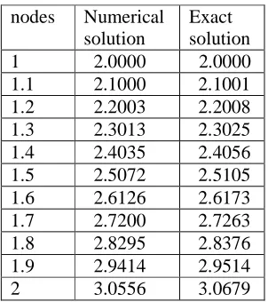
obtained numerical solution is good agreement with the exact solution and the applicability of present method is proved. These solutions are presented in Table1. Solutions for numerical Example 1.
Table 1: Comparison of Exact and Numerical
Table 2: Maximum relative error corresponding number of collocation points
Table 2 presents the number of collocation points and maximum relative error. It is observed from the table 2 that increase in number of collocation points reduce the maximum absolute relative error. This shows convergence of the present method unconditionally.
Example 2.
Third degree Euler-Cauchy differential equation is considered [7] for the applicability of the present proposed numerical method under the various order boundary value problems.
1 ) 1 ( '' 1
) 1 ( ' , 0 ) 1 ( 0
20 20
2 2 2 10 3 3
3 + − + U = withU = U =− andU =
dx dU x dx
U d x dx
U d x
The exact solution is U x x x
11 8 10 44
1 2 4
3 + − +
−
= .
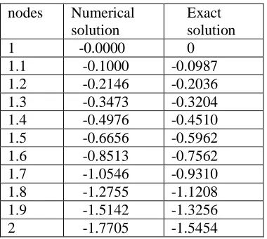
Present numerical method is implemented to the third order Euler –Cauchy equation. The obtained solution is compared with exact solution and presented in Table3. Clearly from
nodes Numerical solution
Exact solution 1 2.0000 2.0000 1.1 2.1000 2.1001 1.2 2.2003 2.2008 1.3 2.3013 2.3025 1.4 2.4035 2.4056 1.5 2.5072 2.5105 1.6 2.6126 2.6173 1.7 2.7200 2.7263 1.8 2.8295 2.8376 1.9 2.9414 2.9514
2 3.0556 3.0679
Number of collocation points
11 21 41 91 201 501
Maximum Relative Error
Using B-Spline Collocation Method
5
the table 3, the numerical solution is close to the exact solution. The proposed third degree B-spline collocation solution is applicable to solve up to the third order boundary value problems.
The increase in number of collocation points improve the exactness of the solution which is shown in the Figure1.It is observed from the figure1 that the present numerical solutions guarantees the convergence when increased the number of collocation points.
Table 3: Comparison of Numerical and Exact solutions
Figure 1: Comparison of numerical and exact solutions for 101colloation points 4. Conclusion
The proposed numerical method is examined to develop numerical solution for Euler-Cauchy boundary value problems by considering numerical examples. The obtained numerical solutions are compared with available exact solutions which are available in
1 1.2 1.4 1.6 1.8 2
-1.6 -1.4 -1.2 -1 -0.8 -0.6 -0.4 -0.2 0
x
U
Numerical solution Exact solution
nodes Numerical solution
Exact solution
1 -0.0000 0
6
literature. The numerical solution is close to exact values and further more applying this method is very easy and simple when compared with the well established numerical methods. This method can be applied to different types of boundary value problems.
REFERENCES
1. T.J.R.Hughes, J.A.Cottrell and Y.Bazilevs, Isgeometric analysis: CAD, finite elements, NURBS, exact geometry and mesh refinement, Comput.Methods Appl. Mech. Engg., 194 (39–41) (2005) 4135–4195.
2. D.F.Rogers and J.Alan Adams, Mathematical Elements for Computer Graphics, 2nd ed., Tata McGraw-Hill Edition, New Delhi.
3. C.de Boor and K. H¨ollig, B-splines from parallelepipeds. J. Analyse Math., 42 (1982) 99– 15.
4. E.Kreyszig, Advanced Engineering Mathematics, Willey (2006).
5. M.L.Abell and James P.Braselton, Introductory Differential Equation with Boundary Value Problems, Acadamic Press, Elsevier 2010.
6. J.K.Zhou, Differential Transformation and its application for electrical circuits’’, Huarjung University Press, Wuuhahn, China (1986).
7. S.O.Edeki, A.A.Opanuga, H.I.Okagbueand G.O.Akinlabi, A numerical-computational technique for solving transformed cauchy-euler equi dimensional equations of homogeneous type, Advanced Studies in Theoretical Physics, 9 (2) (2015) 85-92.