Vol. 7, No. 1, 2014, 47-52
ISSN: 2279-087X (P), 2279-0888(online) Published on 9 September 2014
www.researchmathsci.org
47
Annals of
Multi-objective Cost Varying Transportation Problem
using Fuzzy Programming
Subhrananda Goswami1, Arpita Panda2 and Chandan Bikash Das3
1
Department of Computer Sc. & Engineeing
Haldia Institute Of Technology, Haldia,Purba Midnapore, West Bengal, India email: [email protected]
2
Department of Mathematics, Sonakhali Girls‘s High School, Sonakhali Paschim Midnapore, West Bengal, India
3
Department of Mathematics
Tamralipta Mahavidyalaya, Tamluk, Purba Midnapore-721636, West Bengal, India [email protected]
Received 4 August 2014; accepted 24 August 2014
Abstract. In this paper we represent a multi-objective transportation problem whose transportation cost is varying due to capacity of 2 -vehicles as well as transport quantities. The 2-vehicle multi-objective cost varying transportation problem is a Bi-level Mathematical programming model. To solve this model, use north west corner rule for determining initial basic feasible solution and then set up unit cost (which varies in each iteration) for each cost matrix corresponding to each objective by proper choice of vehicles with our proposed algorithm. Apply optimality test for determining optimal solution for each objective separately. Then apply fuzzy programming technique to sole this model. Numerical examples are presented to illustrate the model.
Keywords: Transportation Problem, Basic Cell, Non-basic Cell, North West Corner Rule AMS Mathematics Subject Classification (2010): 90B
1. Introduction
Transportation problem is a special class of linear programming problem which deals with the distribution of single commodity from various sources of supply to various destination of demand in such a manner that the total transportation cost is minimized. in order to solve a transportation problem, the decision parameters such as availability, requirement and the unit transportation cost of the model must be fixed at crisp values but in real life applications unit transportation cost may be vary due to capacity of vehicles which are transport the commodities from sources to destinations according their demands.
48
then set up unit cost (which varies in each iteration) for each cost matrix corresponding to each objective by proper choice of vehicles with our proposed algorithm. Apply optimality test for determining optimal solution for each objective separately. Then apply fuzzy programming technique to solve this model.
2. Mathematical formulation
A multi-objective transportation problem can be stated in Model 1 as follows:
Model 1
k r
x cr ij
ij n j m i
, 1, = , min
1 = 1 =
…
∑
∑
m i
a x to
subject ij i m
i
, 1, = , =
1 =
…
∑
(1)n j
b xij j n
j
, 1, = , =
1 =
…
∑
(2)j n j i m i
b a
∑
∑
1 = 1 =
= ; xij ≥0 ∀i, ∀j
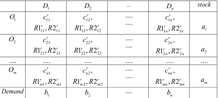
2.2. 2-Vehicle cost varying transportation problem
Suppose there are two types off vehicles V1,V2 from each source to each destination. Let
1
C and C2(>C1) are the capacities(in unit) of the vehicles V1 and V2 respectively. k
r R R
R r
ij r ij r
ij =( 1 , 2 ), =1,…, represent transportation cost for each cell ( ji, ); where
k r
R1ijr, =1,…, are the transportation cost from source O i m
i, =1,…, to the
destination Dj, j=1,…,n by the vehicle .
1
V And R2ijr,r=1,…,k are the transportation cost from source Oi,i=1,…,m to the destination D j n
j, =1,…, by the
vehicle V2. So, for each r=1,…,k cost varying transportation problem can be represent in the following tabulated form.
D1 D2 .. Dn stock
1
O
r c11
r r
R R111, 211
,
12
r c
r r
R R112, 212
....
.... 1 ,
r n c
r n r
n R R11 , 21
1
a
2
O
r c21
r r
R R121, 221
,
22
r c
r r
R R122, 222
....
.... 2 ,
r n c
r n r
n R R12 , 22
2
a
.... .... .... .... .... ....
m O
r n c1
r m r m R R1 1, 2 1
,
2
r n c
r m r m R R1 2, 2 2
....
.... ,
r nn c
r mn r mn R R1 , 2
m a
Demand
1
b b2 .... bn
Multi-objective Cost Varying Transportation Problem using Fuzzy Programming
49
where cijri=1,…,m; j=1,…,n;r=1,…,k are not constants.
2.2.1. Algorithm(CVTP)
Step 1. Since unit cost is not determined (because it depends on quantity of transport), so North-west corner rule (because it does not depend on unit transportation cost) is applicable to allocate initial B.F.S.
Step 2. After the allocate xijr by North-west corner rule, for basic cell we determine cijr (unit transportation cost from source Oi to destination Dj) as
k r
x if
x if x
R p R p
c
ij ij ij
r ij ij r ij ij r
ij =1, ,
0 = 0
0 ,
2 2 1 1
= …
≠ +
(3)
, 1, = ; , 1, = , 2 ,
1 p i m j nareintegersolutionof p
where ij ij … …
r ij ij r ij
ijR p R p1 1 2 2
min + , s.t. xij≤ p1ijC1+p2ijC2
Step 3. For non-basic cell ( ji, ) possible allocation is the minimum of allocations in ith row and jth column (for possible loop). If possible allocation be xijr, then for non-basic cell cijr (unit transportation cost from source Oi to destination Dj) as
k r
x if
x if x
R p R p
c
ij ij ij
r ij ij r ij ij r
ij =1, ,
0 = 0
0 ,
2 2 1 1
= …
≠ +
(4)
, 1, = ; , 1, = , 2 ,
1 p i m j nareintegersolutionof p
where ij ij … …
r ij ij r ij
ijR p R p1 1 2 2
min +
2
1 2
1
.
.t x p C p C
s ij≤ ij + ij
In this manner we convert cost varying transportation problem to a usual transportation problem but cijr is not fixed, it may be changed (when this allocation will not serve optimal value) during optimality test.
Step 4. During optimality test some basic cell changes to non-basic cell and
some non-basic cell changes to basic cell, depends on running basic cell we first fix k
r
cijr, =1,…, by Step 2 and for non-basic we fix c r k
r
50
2.2.2. Bi-level mathematical programming for 2-vehicle multi-objective cost varying transportation problem
The Bi-level mathematical programming for 2-vehicle multi-objective cost varying transportation problem is formulated in Model 2 as follows:
Model 2
k r
x c ij
r ij n j m i
, 1, = , min
1 = 1 =
…
∑
∑
(5)g programmin al
mathematic following
by determined is
c where r
ij
,
k r
x if
x if x
R p R p
c
ij ij ij
r ij ij r ij ij
r
ij =1, ,
0 = 0
0 ,
2 2 1 1
= …
≠ +
r ij ij r ij
ijR p R p1 1 2 2
min + (6)
2
1 2
1
.
.t x p C p C
s ij ≤ ij + ij
m i
a xij i m
i
, 1, = , =
1 =
…
∑
, xij bj j nn j
, 1, = , =
1 =
…
∑
j n j i m i
b a
∑
∑
1 = 1 =
= , xij≥0 ∀i, ∀j
, 1, = ; , 1, = , 2 ,
1 p i m j nareintegersolutionof p
where ij ij … …
2.3. Solution procedure of 2-Vehicle Multi-objective Cost Varying Transportation Problem(TVMOCMTP).
To solve Model 2 first we determine xijr,r−1,…,k for basic each cell ( ji, ) then, determined cijr,r−1,…,k for basic each cell ( ji, ) and for non-basic cell (i,j) (by possible allocation of loop) through Algorithm ) with the help of C-programming then TVMOCMTP converted in linear programming Model 3 with varying unit cost cijras follows:
2.3.1. Linear Programming Formulation of TVMOCMTP
A TVMOCMTP can be stated in Model 3 as follows:
Model 3
k r
x c
Z ij
r ij n j m i
r , =1, ,
min
1 = 1 =
…
∑
∑
Multi-objective Cost Varying Transportation Problem using Fuzzy Programming 51 m i a x to
subject ij i n j , 1, = , = 1 = …
∑
; xij bj j nm i , 1, = , = 1 = …
∑
; j n j i m i b a∑
∑
1 = 1 == ; xij ≥0 ∀i, ∀j
The subscript on Zr and superscript on cijr denote the rth varying unit cost.
Using a linear membership function, the crisp model can be simplified in Model 4 as follows:
Model 4
λ
max (8) k r U L U Z to
subject r+
λ
( r − r)≤ r, =1,…,m i
a xij i n j , 1, = , = 1 = …
∑
; xij bj j nm i , 1, = , = 1 = …
∑
j n j i m i b a∑
∑
1 = 1 == ;xij ≥0 ∀i, ∀j,
λ
≥0where Ur and Lr are the maximum and minimum value of Zr, r=1,2...,k
3. Numerical example
Consider a 2-vehicle cost varying transportation problem as
1
D D2 D3 stock
1
O 5,7 4,6 8,10 14
2
O 2,3 6,8 7,9 16
3
O 3,4 10,12 4,6 12
Deman d
10 15 17
Table 3.1: Table 3.2:
Using our proposed Algorithm , if we consider Table-3.1 as a single objective
2-vehicle cost varying transportation problem then optimal solution is given by
7} = 0, = 0, = 10, = 0, = 6, = 0, = 10, = 4, = {
= 133
1 32 1 31 1 23 1 22 1 21 1 13 1 12 1 11 1 x x x x x x x x x x 4 5 = 1 11 c , 10 4 = 1 12 c , 4 8 = 1 13 c , 1 1 21 3 1 =
c , c122 =1,
10 7 = 1 23 c , 2 1 = 1 31 c , 7 10 = 1 32 c , 7 4 = 1 33 c
Again using our proposed Algorithm, if we consider Table-3.2 as a single objective 2-vehicle cost varying transportation problem then optimal solution is given by
0} = 40, = 0, = 0, = 15, = 45, = 70, = 0, = 5, = {
= 112 122 132 212 222 232 312 322 332
2 x x x x x x x x x x 1 = 2 11 c , 4 11 = 2 12 c , 4 12 = 2 13 c , 3 4 = 2 21
c , c222 =1,
2 1 = 2 23 c , 7 15 = 2 31 c , 6 7 = 2 32 c , 7 4 = 2 33 c 1
D D2 D3 stock
1
O 10,12 11,13 12,14 14
2
O 8,10 6,9 5,7 16
3
O 15,18 14,16 4,6 12
52 Also ( 1)=22
1 x
Z , ( 2)=31.1
1 x
Z , ( 1)=48.5
2 x
Z , ( 2)=36
2 x
Z
Solve by Model 4 by Lingo-13 package. The optimal solution of the problem is 12} = 0, = 0, = 5.0, = 7.84929, = 3.150706, =
0, = 7.150706, =
6.849294, =
{
= 11 12 13 21 22 23 31 32 33
*
x x x x x
x x x
x x
30.67857 =
* 1
Z *=47.92111
2
Z
λ
*=0.04634. Conclusion
In this paper we have developed two-vehicle multi-objective cost varying transportation problem. We transfer this multi-objective cost varying transportation problem to usual multi-objective transportation problem by Northwest corner rule and then apply optimality test where unit transportation cost vary from one table to another table. This problem is more real life problem than usual transportation problem.
REFERENCES
1. F.L.Hitchcock, The distribution of a product from several sources to numerouslocalities, Journal of Mathematical Physics, 20(17) (1941) 224–230. 2. G.B.Dantzig, Linear Programming and Extensions, Princeton University Press,
Princeton, (1963).
3. H.A.Taha, Operation Research: An Introduction, Macmillan, New York, (1992). 4. H.J.Zimmermann, Fuzzy programming and linear programming with several
objective functions, Fuzzy Sets and Systems, 91(1) (1997) 37–43.
5. H.J.Zimmermann, Fuzzy Set Theory and its Applications, 4th ed., Kluwer-Nijhoff, Boston, (2001).
6. A.Panda and C.B.Das, 2-vehicle cost varying transportation problem, Journal of Uncertain Systems, 8(1) (2014) 44–57.
7. A.Panda and C.B.Das, Capacitated Transportation Problem under Vehicles, LAPLAMBERT Academic Publisher, Deutschland/Germany, (2014).
8. A.Panda and C.B.Das, N-vehicle cost varying transportation problem, Advanced Modeling and Optimization, 15( 3) (2013) 583–610 .
9. A.Panda, C.B.Das, Cost varying interval transportation problem under 2-vehicle, Journal of New Results in Sciences, 3(3) (2013) 19–36.
10. A.Panda and C.B.Das, N-vehicle cost varying capacitated transportation problem, Ciit-international Journal of Fuzzy Systems, 5(7) (2013) 191-204.