A MEMS-based smart sensor system for estimation of camera pose for computer

(1)

A MEMS-based Smart Sensor System for Estimation of Camera Pose for Computer

Vision Applications

Dominik Aufderheidea,b, Werner Krybusa, Dennis Doddsb

a_{South Westphalia University of Applied Sciences, Division Soest}

Institute for Computer Science, Vision and Computational Intelligence Luebecker Ring 2, 59494 Soest, Germany

E-Mail: {aufderheide, krybus}@fh-swf.de

b_{The University of Bolton, School of the Built Environment and Engineering}

Deane Road, Bolton BL3 5AB, U.K. E-Mail: {dma1bee, d.dodds}@bolton.ac.uk

Abstract

The estimation of a cameras egomotion during image acquisition is a mandatory task for many different computer vision applications such as Structure from Motion (SfM), Simultaneous Localisation and Mapping (SLAM) or Augmented Reality (AR). The vast majority of the proposed applications are deriving the motion parameters indirectly from the captured images. This paper suggests a smart sensor system (S3) composed from three different micro-electromechanical (MEMS) inertial sensor types as an aiding modality for vision-based camera pose estimation. The S3 implementation contains a signal conditioning unit and a bank of Kalman filters for orientation estimation. The whole system is evaluated by using an industrial robot for the generation of specific motion patterns and the corresponding ground truth orientation measurements.

Keywords: Kalman ﬁlter, MEMS, Smart Sensor Systems, Inertial Navigation, Multi-Sensor Data Fusion,

Camera Egomotion Estimation

1. Introduction

For many different algorithms in the field of com-puter vision (CV) it is necessary to determine the absolute or relative pose (position and orientation) of the camera during the acquisition of a monocu-lar image stream. In most cases the computed pose of the camera is a prerequisite for further computa-tions. One prominent example is the field of Struc-ture from Motion (SfM) which realises the simultane-ous estimation of camera egomotion and computation of a three dimensional representation of an observed scene based on the captured image sequence. A de-tailed description of the SfM procedure is given e.g. in Pollefeys et al. [1998], Poelman and Kanade [1997]. Another example is the field of mobile robotics where methods for simultaneous localisation and mapping (SLAM) are recently developed which allow on the one hand the localisation of a single moving robot platform based on image frames (Visual Odometry -VO) and on the other hand the synchronous mapping of the robots environment. Prominent examples can

be found in Davison and Kita [2002] and Pupilli and Calway [2006]. Closely related is the ﬁeld of parallel tracking and mapping (PTAM) which was initially solved by Klein and Murray [2007] for applications in Augmented Reality (AR). AR is also a typical ex-ample for the usage of the camera pose in CV appli-cations. The general idea of many AR applications is the placement of 3D computer generated graphics (CGI) in a video captured by a standard camera. The perspective view of the 3D CGI model has to be ren-dered based on the actual position of the camera to generate a natural appearance of the artiﬁcial object. Examples of such procedures can be found e.g. in Schmalstieg and Wagner [2007].

(2)

(PoIs) are detected by diﬀerent PoI detectors sug-gested in literature, such as Harris-features (Harris and Stephens [1988]), SIFT-features (Lowe [2004]) or SURF-features (Bay et al. [2008]).

For tracking and matching many different frameworks were suggested in literature during the last decades, whereat it is possible to distinguish between those ap-proaches which rely only on a small subset of anchor features or those which try to maximise the num-ber of point features even if there is the possibil-ity for the generation of wrong matches (outliers). These two different approaches emphasise different subtasks, while for anchor feature approaches sophis-ticated tracking mechanisms (e.g. Hidden Markov Models (HMM) as suggested by Xie and Evans [1990]) have to be implemented, it is mainly necessary to include routines for outlier handling for the other al-ternative (e.g. Random Sample Consensus (RanSaC) Nister [2003]). Nevertheless the prerequisite of reli-able feature tracks is often very hard to accomplish, because the feature matching between successive frames suffers from problems such as motion blur, perspec-tive projection, repetiperspec-tive patterns, less textured ar-eas, computational complexity, etc. In Aufderheide et al. [2009] and Steffens et al. [2009] different typical problems classes of point registration are identified. Especially for long-time sequences the robust track-ing of natural landmarks is an almost open question in the computer vision community.

This paper suggests a smart sensor system (S3) com-posed as a bank of diﬀerent micro-electromechanical systems (MEMS). The proposed system contains ac-celerometers, gyroscopes and magnetometers. All of them are sensory units with three degrees of freedom (DoF). TheS3 contains the sensors itself, signal con-ditioning (ﬁltering) and a multi-sensor data fusion (MSDF) scheme for orientation estimation.

The performance of the system is evaluated by using diﬀerent motion patterns generated by an industrial robot. This allows the generation of ground truth data. The system was compared against other possi-ble fusion schemes.

The remainder of this paper is organised as follows: Section 2 describes the general architecture of the proposed S3. The following Sections introduce the diﬀerent stages of the system, namely hardware (Sec-tion 3), signal condi(Sec-tioning (Sec(Sec-tion 4) and Sensor Fusion (Section 5). An overview about the experi-mental evaluation of the system is given in Section 6. Finally Section 7 concludes the whole paper and

shows possible future work.

2. General S3 architecture

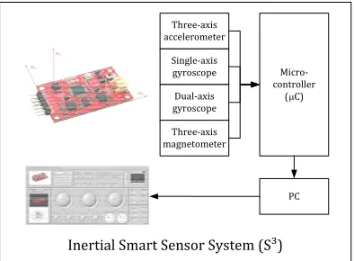
The general architecture of the S3 is shown in the following Figure 1. Whereat the overall architec-ture contains mainly the sensory units as described in subsection 3.1. A single micro controller is used for analog-digital-conversion (ADC), signal conditioning (SC) and transfer of sensor data to a PC (see Section 4). The actual sensor fusion scheme, as described in Section 5, for the estimation of orientation is realised in the PC for a better visualisation.

ȋͿȌ

Ǧ

ȋ Ȍ

Figure 1: General architecture of the inertialS3

3. Hardware

The main hardware which is used to build the

S3 is of course the bank of inertial sensory units in MEMS technology. An additional micro controller (μC) was added mainly for signal conditioning pur-poses.

3.1. Sensory units

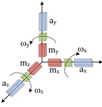
The general architecture of the proposed S3 sys-tem is based on three diﬀerent types of inertial mea-surement units (IMUs). The whole system consist of three orthogonal arranged accelerometers which mea-sure a three dimensional accelerationab = [axayaz]T

and three gyroscopes which measure the angular ve-locities ωb = [ωxωyωz]T around the sensitivity axes

of the accelerometers. As an addition three magne-tometers are able to determine the earth magnetic ﬁeld in 3 DoF mb = [mxmymz]T. All of the

(3)

rigidly attached to the IMU-platform. The following ﬁgure shows the general conﬁguration of all sensory units and the corresponding measured entities.

Figure 2: General architecture of the IMU

Due to the fact that the whole unit should be available for low-costs only oﬀ-the-shelf sensors are used, whereat a single-axis gyroscope LY530AL and a LPR530AL dual-axis gyroscope from STMircoelec-tronics are used to measure the angular velocities around all three axes. Analog Devices provides with the ADXL345 a full 3-DoF accelerometer unit in a single chip. For measuring the earth’s magnetic ﬁeld, Honeywell provides a 3-DoF magnetometer (HMC5843).

3.2. Processing units

The diﬀerent sensory units are connected to the micro controller by using eitherI2C-Bus (Accelerom-eter and Magnetom(Accelerom-eter) or direct ADC of voltage output signals (Gyroscopes). Due to the diﬀerent shape of the signals the complete signal conditioning was placed inside the μC in digital domain. We use a ATMega 328 processor from AVR to collect data from all information channels and subsequent signal conditioning and transfer by USB to the PC.

4. Sensor Modelling and Signal Conditioning

Measurements from MEMS devices in general and inertial MEMS sensors in particular are suﬀering from diﬀerent error sources. Due to this it is necessary to implement both an adequate calibration routine and a signal conditioning routine.

The calibration of the sensory units is only possible if a reasonable sensor model is available beforehand.

The sensor model should address all possible error sources. Here the proposed model from Skog and H¨andel [2006] was utilised and adapted for the given context. It can be shown that the main inﬂuences for the occurrence of measurement errors are the follow-ing (see Petkov and Slavov [2010]):

• Misalignment of sensitivity axes - Ideally the three independent sensitivity axes of the sen-sory should be orthogonal. Due to imprecise construction of MEMS-based IMUs this is not the case for the vast majority of sensory pack-ages. The misalignment can be compensated by ﬁnding a matrixM which transforms the non-orthogonal axis to a non-orthogonal setup as shown in Dorobantu [1999].

• Biases - The output of a sensor should be ex-actly zero if the S3 is not moved. Also this is not true, because it was shown e.g. in Gul-mammadov [2009], that there is a time-varying oﬀset. Here Aslan and Saranli [2008] diﬀeren-tiate g-independent biases (e.g. for gyroscopes)

and g-dependent biases. For the later there is

a relation between the applied acceleration and the bias. The bias is modelled by incorporation of a bias vector b

• Measurement noise - Of course also the gen-eral measurement noise has to be taken into ac-count, whereat it is assumed here as a white noise termn.

• Scaling factors - In most cases there is an un-known scaling factor between the measured phys-ical quantity and the real signal. The scaling can be compensated by introducing a scale ma-trixS=diag(sx, sy, sz).

Based on these error classes a general error-model based on the findings in Skog and Händel [2006] was used in this work. The general model is valid for the different inertial sensors. A block-diagram of the general sensor model is shown in the following figure.

ȋǦȌ

н

ȋǦȌ

(4)

Based on this it is possible to deﬁne three separate sensor models for all three sensor types1, as shown in the following equations:

ωb=Mg·Sg·ωb +bg+ng (1)

ab =Ma·Sa·ab+ba+na (2)

mb =Mm·Sm·mb+bm+nm (3)

It was shown that M and S can be determined by sensor calibration routines which move the sensor array to diﬀerent known locations to determine the calibration parameters. So presented Hwangbo [2008] a calibration approach based on the factorisation of a measurement matrix which is inspired by method-ologies from classical SfM.

The noise and the bias terms can not be determined a-priori due to their time-varying character. The sig-nal conditioning step on the μC takes care of the measurement noise by integrating an FIR digital fil-ter structure. The implementation realises a low-pass FIR filter based on the assumption that the frequen-cies of the measurement noise are much higher than the frequencies of the signal itself. The complete fil-ter was realised in software on the μC, whereat the different cutoff-frequencies for the different sensory units were determined in an experimental evaluation. Based on the conditioned signals is it now possible to fuse the measurements from the different sensors for attitude estimation as described in the next section.

5. Multi-Sensor Data Fusion

The general idea of the multi-sensor data fusion (MSDF) step is based on the redundancy in the mea-surements delivered by the bank of inertial sensors. This is important, because due to the immense inﬂu-ence of noise and biases it is not possible to rely only on one source of information. In MSDF it is possi-ble to interpret the diﬀerent sensors as independent information channels, as suggested by Mitchell [2007].

Classical approaches for inertial navigation are stable-platform systems which are isolated from any exter-nal rotatioexter-nal motion by specialised mechanical forms. In comparison to those classical stable plat-form systems the MEMS sensors are mounted rigidly

1_{The diﬀerent sensor types are indicated by the subscript}

indices at the entities in the diﬀerent equations.

MODS

Signal Conditioning

Accelerometers

Gyroscopes

Magnetometers

ab

Zb

mb

Orientation estimation

Initial orientation Coordinate

transform Cn

b

;

Position estimation Gravity correction g

Orientation Initial position

and speed

Position

Figure 4: Computational elements of an INS

to the device (here: the camera). In such a strap-down system it is necessary to transform the mea-sured quantities of the accelerometers into a global coordinate system by using known orientations com-puted from gyroscope measurements. In general the mechanisation of a strapdown inertial navigation sys-tems (INS) can be described by the computational elements indicated in Figure 4. The necessary com-putation of the orientation ξ of the S3 based on the gyroscope measurements ωb and a start orientation

ξ₍t0) can be described as follows:

ξ=ξ₍_t₀₎+

ωbdt (4)

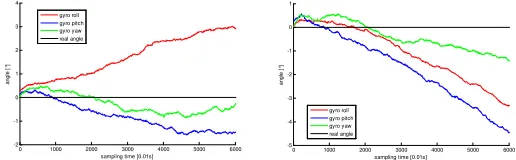
The integration of the measured rotational velocities would lead to an unbounded drifting error in the ab-solute orientation estimates. Figure 5 shows two ex-amples for this typical drifting behaviour for all three Euler angles. For the two experiments shown in Fig-ure 5 the S3 was not moved, but even after a short period of time (here: 6000·0.01s= 60s) there is an absolute orientation error of up to 4 recognisable. For

0 1000 2000 3000 4000 5000 6000 -5

-4 -3 -2 -1 0 1

sampling time [0.01s]

a

ngl

e [

°]

gyro roll gyro pitch gyro yaw real angle 0 1000 2000 3000 4000 5000 6000

-2 -1 0 1 2 3 4

a

ngl

e [

°]

gyro roll gyro pitch gyro yaw real angle

Figure 5: Drifting error for orientation estimates based on gy-roscope measurements

(5)

inertial reference frameai only by double integration:

ϕ=ϕ₍t₀)+ aidt (5)

On the other hand possible errors in the orientation estimation stage would lead also to a wrong position due to the necessity to transform the accelerations in the body coordinate frameabto the inertial reference

frame (here indicated by the subscript i).

The following ﬁgure gives an impression about the typical drifting error for the absolute position (one axis) computed by using the classical strapdown method-ology. It can be easily seen that after 20 s the error is already drifted to approximately 13 m for a not moved device.

6DPSOLQJ7LPH>V@

D[ DFFHOHUDWLRQ

6DPSOLQJ7LPH>V@

V[ SRVLWLRQ

Figure 6: Drifting error for absolute position estimates based on classical strapdown mechanisation of an inertial navigation system (left: acceleration measurements; right: absolute posi-tion estimate)

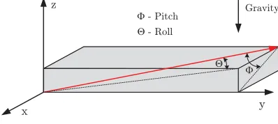
By using only gyroscopes there is actually no pos-sibility to bound the drifting error for the orientation in a reasonable way. At this point it is necessary to use other information channels. The general idea for compensating the drift error of the gyroscopes is based on using the accelerometer as an additional at-titude sensor for generating redundant information. Due to the fact that the 3-DoF accelerometer mea-sures not only (external) translational motion, but also the inﬂuence of the gravity it is possible to cal-culate the attitude based on the single components of the measured acceleration. This is of course only true if no external force is accelerating the sensor. So there are to questions which have to be answered: 1. How it is possible to calculate the attitude from accelerometer measurements? and 2. How external translational motion can be handled? Both problems can be solved by following a two-stage switching be-haviour inspired by work presented in Rehbinder and Hu [2004]. At this point it should be pointed out that measurements from the accelerometers can only pro-vide roll and pitch angle and the heading angle has to be derived by using the magnetometer instead.

INERTIAL FUSION CELL (IFC)

y z

x

4- Roll )- Pitch

) 4

Gravity

Figure 7: Geometrical relations between measured accelera-tions due to gravity and the roll and pitch angle of the attitude

Figure 7 gives an illustration about the geometrical relations between measured accelerations due to grav-ity and the roll and pitch angle of the attitude. By this it follows that the angles can be determined by following relations:

θ=arctan2

a2_x,

(ay+az)2

(6)

φ=arctan2

a2_y,(ax+az)2

(7)

The missing heading angle can be recovered by using the readings from the magnetometer and the already determined roll and pitch angles. Here it is important to consider that the measured elements of the earth magnetic ﬁeld have to be transformed to the local horizontal plane (tilt compensation). Figure 8 is indicating the corresponding relations as shown in Caruso [2000]:

Xh =mx·cϕ+my·sθ·sϕ−mz·sθ·sϕ

Yh =my·cθ+mz·sθ

ψ= arctan 2 (Yh, Xh)

(8)

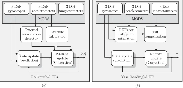
Based on these ﬁndings a discrete Kalman ﬁlter bank (DKF-bank) is implemented which is responsi-ble for the estimation of all three angles ofΞ. For the pitch and the roll angle the same DKF-architecture is used, as indicated in Figure 9-(a). In comparison to that the heading angle is estimated by a alternative architecture as shown in Figure 9-(b).

Local horizontal plane

Gravity -roll

pitch

Yh

Xh

(6)

Yaw (heading)-DKF Roll/pitch-DKFs

MODS 3 DoF accelerometers 3 DoF

gyroscopes

3 DoF magnetometers

State update (prediction)

Kalman update (Correction) Attitude calculation External

acceleration detector

TI

MODS 3 DoF accelerometers 3 DoF

gyroscopes

3 DoF magnetometers

State update (prediction)

Kalman update (Correction)

Tilt compensation DKFs for

roll/pitch estimation

\

(a) (b)

Figure 9: (a) - Discrete Kalman ﬁlter (DKF) for estimation of roll and pitch angles based on gyroscope and accelerometer measurements; (b) - DKF for estimation of yaw (heading) angle from gyroscope and magnetometer measurements

All DKFs are mainly based on the classical structure of a Kalman ﬁlter (see Bishop [2007]) which consists of a ﬁrst prediction of states and subsequent correc-tion, where the two states are the unknown angle ξ

and the bias of the gyroscope bgyro. The Kalman

ﬁl-tering itself is composed from the following classical steps, whereat the following descriptions are simpli-ﬁed to a single angle ξ.

5.1. Computation of an a priori state estimate x−_k₊₁

As already mentioned the hidden states of the sys-tem are x = [ξ,bgyro]T. The a priori estimates are

computed by following the following relations:

ωk+1=ωk+1−bgyrok

ξk+1=ξk+

ωk+1dt

bgyrok+1 =bgyrok

(9)

Here the actual measurements from the gyroscopes

ωk+1 are corrected by the actually estimated bias bgyrok from the former iteration, before the actual

an-gle ξk+1 is computed.

5.2. Computation of a priori error covariance matrix P−_k₊₁

The a priori covariance matrix is calculated by incorporating the Jacobi matrix A of the states and the process noise covariance matrix QK as follows:

P−_k₊₁=A·Pk·AT+QK (10)

The two steps 1) and 2) are the elements of the prediction step as indicated in Figure 9.

5.3. Computation of Kalman gainKk+1

As a prerequisite for computing the a posteriori state estimate the Kalman gain Kk+1 has to be

de-termined by following Equation 11.

Kk+1=P−_k₊₁·HTk+1·

Hk+1·P−k+1·HTk+1+Rk+1

−1 (11)

5.4. Computation of a posteriori state estimatex+_k₊₁

The state estimate can now be corrected by using the calculated Kalman gain Kk+1. Instead of

incor-porating the actual measurements as in the classical Kalman structure the suggested approach is based on the computation of an angle diﬀerence Δξ. The dif-ference is a comparison of the angle calculated from the gyroscope measures and the corresponding atti-tude as derived from the accelerometers, respectively the heading angle from the magnetometer, as already introduced in the introduction of this chapter. So the relation forx+_k₊₁ can be formulated as:

x+_k₊₁ =x−_k₊₁−Kk+1·Δξ (12)

At this point it is important to consider the fact that the attitude measurements from the accelerometers are only reliable if there is no external translational motion. For this an external acceleration detection mechanism is also part of the fusion procedure. For this reason the following condition (see Rehbinder and Hu [2004]) is evaluated continuously:

a=

(7)

If the relation is fulfilled there is no external accel-eration and the estimation of the attitude from ac-celerometers is more reliable than the one computed from rotational velocities as provided by the gyro-scopes. Noteworthy for real sensors an adequate thresh-old g is introduced to define an allowed variation from this ideal case. If the camera is not at rest the observation variance for the gyroscope data σ_g2 is set to zero. So by incorporating the magnitude of the ac-celeration measurements as a and the earth gravi-tational fieldg= [0,0,−g]T the observation variance can be defined by following Equation 14.

σ_g2 =

σ2_g,

0,

a − g< εg

otherwise (14)

A similar approach is chosen to overcome the prob-lems with the magnetometer measurements in mag-netically distorted environments for the DKF for the heading angle. Instead of gravity gthe magnitude of the earth magnetic ﬁeld m is evaluated as shown in the following relation2:

σ_g2=

σ2_g,

0,

m −mdes< εm

otherwise (15)

5.5. Computation of posteriori error covariance ma-trixP+_k₊₁

Finally the error covariance matrix is updated in the following way:

P+_k₊₁=P−_k₊₁−Kk+1·Hk+1·P−k+1 (16)

6. Results

as already mentioned our approach was evaluated by using an ABB IRB1400 industrial robot. The S3

was attached to the robot and moved along prede-ﬁned motion patterns. Thus the ground truth data of the movement is available for a comparison. The tests consider besides the comparison against ground truth also a comparison against other iner-tial navigation algorithms:

• Gyroscopes alone (Gyro) - Here we tested

the naive implementation of a simple integra-tion of gyroscope measures as indicated in Equa-tion 4, whereat the initialisaEqua-tion of the starting orientation was computed by using accelerome-ter and magnetomeaccelerome-ter measurements.

2_m

desdescribes the magnitude of the earth’s magnetic ﬁeld

(e.g. 48µT in Western Europe)

• Complementary Filtering (CF) - The CF

approach as suggested by Euston et al. [2008] or Baerveldt and Klang [1997] combines the two information channels (gyroscopes and accelerom-eters) by using a simple adder, but the two signal sources are filtered before by two com-plimentary filters. So the accelerometer mea-surements are filtered by a low-pass filter (here: first-order) and the gyroscope signals by a high-pass filter.

• Weighting Filter (Est) - The weighting

ﬁl-ter approach as suggested by Bluemel [2010] is a simple straightforward combination of ac-celerometer and gyroscope measurements by us-ing ﬁxed weights.

For the test diﬀerent motion patterns were used: ro-tation around a single axis, consecutive roro-tation around two axis and simultaneous rotation around two axes. The following subsections summarise the results of the comparison.

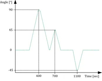
6.1. Rotation around a single axis

The ﬁrst motion pattern contains rotations of the roll/pitch angle as indicated in the following ﬁgure. The motion pattern was tested for the roll and pitch

ȏȐ ȏιȐ

ͻͲ

Ͷͷ

ǦͶͷ Ͳ

ͶͲͲ ͹ͲͲ ͳͳͲͲ

Figure 10: Motion pattern for roll/pitch angle

angle while the orientation estimation was computed by using the suggested method based on a bank of Kalman ﬁlters and the three naive methods described above. All results were tested against the ground truth, thus an absolute error angle was computed for all the algorithms. Figure 11 and Figure 12 show the results of this test for the roll and pitch angle. Here

(8)

0 200 -6 -4 -2 0 2 4 6 8 an gl e [ °] ďď ϭϭ

400 600 800 1000 12

ϭ ϳ ďƐŽůƵƚĞƌ DĞƐƐǁŝŶŬĞůĨĞŚůĞƌ ĚĞƐ ZŽůů tŝŶŬĞůƐ

200 1400

RxEst

gyro roll roll CF KF roll

Figure 11: Absolute orientation error (roll angle) for movement around a single axis

200 -1 0 1 2 3 4 5 6 7 8 9 an gl e [ °]

400 600 800 1000 1

200 RyEst

gyro pitch pitch CF KF pitch

Figure 12: Absolute orientation error (pitch angle) for move-ment around a single axis

The typical drifting behaviour of the gyroscope measures can be directly identiﬁed in the orientation estimates delivered only by gyroscope measures. The suggested KF approach outperforms the other ﬁlter-ing methods.

6.2. Consecutive rotation around two axes

The second motion pattern contains a rotation of 90◦ around the roll-axis and a consecutive rotation of 90◦ around the yaw-axis. The following Figure 13 gives an impression about the performance of the dif-ferent ﬁltering strategies for this kind of motion. It can be seen that especially the CF approach got immense problems during the times of motion. Also for this test the KF approach delivers the best results, but the simple weighting approach delivers compara-ble results but with less computational complexity. The gyroscopes alone show the same drifting results as for the previous experiments.

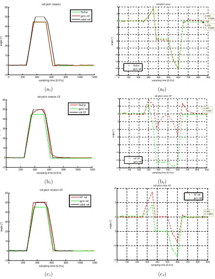
6.3. Simultaneous rotation around two axes

Finally we tested the motion pattern with a si-multaneous movement around two axes. The results are summarised in Figure 14, whereat again a com-parison against the other methods was carried out.

0 200 400 600 800 10001200 14001600 1800 -20 0 20 40 60 80 100

an g le [ °] roll-yaw rotation RxEst gyro roll robot roll

0 200 400 600 800 1000 1200 1400 -10 -5 0 5 10 15

a ngl e [ °] roll-yaw error X: 1300 Y: 10.86 X: 1300 Y: 0.7194 RxEst gyro roll

0 200 400 600 800 1000 12001400 1600 1800 -20 0 20 40 60 80 100 120 140 160 180

a

ngl

e

[

°]

roll-yaw rotation CF

roll CF gyro roll robot roll

0 200 400 600 800 1000 1200 1400 -10 -5 0 5 10 15 X: 1300 Y: 0.4996

a

ngl

e

[

°]

roll-yaw error KF

KF roll gyro roll

0 200 400 600 800 10001200 14001600 1800 -20 0 20 40 60 80 100

an

gl

e

[

°]

roll-yaw rotation KF

KF roll gyro roll robot roll

0 200 400 600 800 1000 1200 1400 -10 -5 0 5 10 15 X: 1300 Y: 0.4996

a

ngl

e

[

°]

roll-yaw error KF

KF roll gyro roll

(a1) (a2)

(b1) (b2)

(c1) (c2)

Figure 13: Comparison of diﬀerent ﬁltering techniques for

consecutive motion pattern - (a1): Orientation estimates for weighting ﬁlter; (a₂): Absolute error for weighting ﬁlter; (b₁): Orientation estimates for CF; (b2): Absolute error for CF; (c1): Orientation estimates for KF; (c2): Absolute error for KF

The suggested KF approach shows the best result in terms of accuracy and long-time stability.

7. Conclusion and future work

It was shown that the suggested approach which utilises a bank of Kalman ﬁlters is able to outperform other classical methods for orientation estimation. In this context it was proved that the usage of a smart sensor system containing a sensor array, signal con-ditioning devices and a sensor fusion scheme is able to deliver reliable information about a cameras pose. This information can be fed into classical computer vision algorithms as an aiding modality for camera egomotion estimation.

(9)

0 200 400 600 800 1000 1200 -10 0 10 20 30 40 50 60

an gl e [ °] roll-pitch rotation RxEst gyro roll robot roll

0 200 400 600 800 1000 1200

-10 0 10 20 30 40 50 60

an

gl

e [

°]

roll-pitch rotation CF

RxEst gyro roll roll CF

0 200 400 600 800 1000 1200

-10 0 10 20 30 40 50 60

a

ngl

e

[

°]

roll-pitch rotation KF

KF roll gyro roll robot roll

0 100 200 300 400 500 600 700 800 900 -15 -10 -5 0 5 10

a

ngl

e [

°]

roll-pitch error KF

X: 850 Y: 0.0223 KF roll gyro roll

(a1) (a2)

(b1) (b2)

(c1) (c2)

0 100 200 300 400 500 600 700 800 900 -16 -14 -12 -10 -8 -6 -4 -2 0 2 4 X: 850 Y: -0.2689

an g le [ °] roll-pitch error X: 850 Y: -0.5382 RxEst gyro roll

0 100 200 300 400 500 600 700 800 900 -14 -12 -10 -8 -6 -4 -2 0 2 4

an

gl

e [

°]

roll-pitch error CF

X: 850 Y: 0.0407

roll CF gyro roll

Figure 14: Comparison of different filtering techniques for si-multaneous motion pattern - (a1): Orientation estimates for weighting filter; (a2): Absolute error for weighting filter; (b1): Orientation estimates for CF; (b₂): Absolute error for CF; (c₁): Orientation estimates for KF; (c2): Absolute error for KF

and Krybus [2011] which contains a visual and an inertial fusion cell.

Acknowledgements

The authors acknowledge support from all other fellows and students at the Laboratory for Image Pro-cessing Soest (LIPS) and the Institute for Computer Science, Vision and Computational Intelligence, es-pecially Mr. Dominik Bluemel for his participation in the project. Furthermore we like to thank all peo-ple at the Electronics Department of the School of the Built Environment and Engineering at the University of Bolton for their kind support.

Authors Biographies

Dominik Aufderheideis an active researcher in the

area of multi-sensor image processing and computer vision. Currently he is a research fellow at the Insti-tute of Computer Science, Vision and Computational Intelligence (CV&CI), where he is working towards a Ph.D. in cooperation with the University of Bolton.

Werner Krybusis a professor for data systems

en-gineering and signal processing at South Westphalia University of Applied Sciences. He is founder of the Laboratory for Image Processing Soest within the In-stitute for Computer Science, Vision and Computa-tional Intelligence. His primary research interests in-clude embedded systems, computer vision and sensor fusion.

Dennis Doddsis an academic teaching fellow at the

University of Bolton. He graduated with a Ph.D. at the University of Salford and gained practical expe-rience in a position as a research engineer at Ferranti Semiconductors Ltd. His research interests can be summarised as non-contacting measurement systems, biomedical and current-mode analogue electronics.

References

M. Pollefeys, R. Koch, M. Vergauwen, L. V. Gool, Gool. Met-ric 3D surface reconstruction from uncalibrated image

se-quences, in: In: 3D Structure from Multiple Images of

Large Scale Environments. LNCS Series, Springer-Verlag, 1998, pp. 138–153.

C. Poelman, T. Kanade, A paraperspective factorization

method for shape and motion recovery, IEEE Transactions on Pattern Analysis and Machine Intelligence 19 (1997) 206– 218.

A. J. Davison, N. Kita, Simultaneous localisation and map-building using active vision, IEEE Transactions on Pattern Analysis and Machine Intelligence (2002) 865–880.

M. Pupilli, A. Calway, Real-time visual slam with resilience to erratic motion, in: CVPR (1), IEEE Computer Society, 2006, pp. 1244–1249.

G. Klein, D. Murray, Parallel tracking and mapping for small ar workspaces, 2007 6th IEEE and ACM International Sym-posium on Mixed and Augmented Reality 07 (2007) 1–10. D. Schmalstieg, D. Wagner, Experiences with handheld

aug-mented reality, 2007 6th IEEE and ACM International Sym-posium on Mixed and Augmented Reality 07pp (2007) 1–13. C. Harris, M. Stephens, A combined corner and edge detector,

volume 15, Manchester, UK, pp. 147–151.

D. G. Lowe, Distinctive image features from scale-invariant

keypoints, International Journal of Computer Vision 60

(2004) 91–110.

H. Bay, A. Ess, T. Tuytelaars, L. V. Gool, Speeded-Up Robust Features (SURF), Computer Vision and Image Understand-ing 110 (2008).

X. Xie, R. Evans, Multiple target tracking using hidden markov models, in: Radar Conference, 1990., Record of the IEEE 1990 International, pp. 625 –628.

D. Nister, Preemptive ransac for live structure and motion es-timation, Proceedings Ninth IEEE International Conference on Computer Vision 16 (2003) 199–206 vol.1.

D. Aufderheide, M. Steﬀens, S. Kieneke, W. Krybus,

(10)

stereo matching by a probabilistic scene analysis, in: Pro-ceedings of the 9th Conference on Optical 3-D Measurement Techniques, Wien, pp. 328–331.

M. Steﬀens, D. Aufderheide, S. Kieneke, W. Krybus,

C. Kohring, D. Morton, Probabilistic Scene Analysis for Robust Stereo Correspondence, in: Lecture Notes In Com-puter Science; Vol. 5627.

I. Skog, P. H¨andel, Calibration of a MEMS inertial measure-ment unit, in: XVII IMEKO World Congress on Metrology for a Sustainable Development, Rio de Janeiro, Brazil. P. Petkov, T. Slavov, Stochastic modeling of mems inertial

sensors, Cybernetics and Information Technologies 10 (2010) 31–41.

R. Dorobantu, Simulation des Verhaltens einer lowcost

Strapdown-IMU unter Laborbedingungen, 1999.

F. Gulmammadov, Analysis, modeling and compensation of bias drift in mems inertial sensors, in: Recent Advances in Space Technologies, 2009. RAST ’09. 4th International Conference on, pp. 591 –596.

G. Aslan, A. Saranli, Characterization and Calibration of Mems Inertial Measurement Units, EURASIP.

M. Hwangbo, Factorization-based calibration method for mems inertial measurement unit, 2008 IEEE International Confer-ence on Robotics and Automation (2008) 1306–1311.

H. Mitchell, Multi-Sensor Data Fusion: An Introduction,

Springer Verlag, Berlin-Heidelberg, 2007.

H. Rehbinder, X. Hu, Drift-free attitude estimation for accel-erated rigid bodies, Automatica 40 (2004) 653 – 659. M. Caruso, Applications of magnetic sensors for low cost

com-pass systems, pp. 177 –184.

C. M. Bishop, Pattern Recognition and Machine Learning (In-formation Science and Statistics), Springer, 2007.

M. Euston, P. Coote, R. Mahony, J. Kim, T. Hamel, A

complementary ﬁlter for attitude estimation of a ﬁxed-wing uav, in: Intelligent Robots and Systems, 2008. IROS 2008. IEEE/RSJ International Conference on, pp. 340 –345. A. J. Baerveldt, R. Klang, A low-cost and low-weight

atti-tude estimation system for an autonomous helicopter, vol-ume pages, IEEE, pp. 391–395.

D. Bluemel, Entwicklung und evaluierung einer inertialen mes-seinheit fuer die robuste schaetzung von kamerabewegungen, 2010.