Algebraic Topology

(1)

Algebraic Topology

John W. Morgan P. J. Lamberson August 21, 2003

Introduction

Algebraic topology is a large and complicated array of tools that provide a framework for measuring geometric and algebraic objects with numerical and algebraic invariants. The original motivation was to help distinguish and eventually classify topological spaces up to homeomorphism or up to a weaker equivalence called homotopy type. But the subject has turned out to have a vastly wider range of applicability. In the cases of the most interest, the objects to which we apply the invariants of algebraic topology arise naturally in geometric, analytic, and algebraic studies. The power of algebraic topology is the generality of its application. The tools apply in situations so disparate as seemingly to have nothing to do with each other, yet the common thread linking them is algebraic topology. One of the most impressive arguments by analogy of twentieth century mathematics is the work of the French school of algebraic geometry, mainly Weil, Serre, Grothendieck, and Deligne, to apply the machinery of algebraic topology to projective varieties defined over finite fields in order to prove the Weil Conjectures. On the face of it these conjectures, which dealt with counting the number of solutions over finite fields of polynomial equations, have nothing to do with usual topological spaces and algebraic topology. The powerful insight of the French school was to recognize that in fact there was a relationship and then to establish the vast array of technical results in algebraic geometry over finite fields necessary to implement this relationship.

Let me list some of the contexts where algebraic topology is an integral part. It is related by deRham’s theorem to differential forms on a manifold, by Poincar´e duality to the study of intersection of cycles on manifolds, and by the Hodge theorem to periods of holomorphic differentials on complex algebraic manifolds. Algebraic topology is used to compute the infinitessimal version of the space of deformations of a complex analytic manifold (and in particular, the dimension of this space). Similarly, it is used to compute the infinitessimal space of deformations of a linear representation of a finitely presented group. In another context, it is used to compute the space of sections of a holomorphic vector bundle. In a more classical vein, it is used to compute the number of handles on a Riemann surface, estimate the number of critical points of a real-valued function on a manifold, estimate the number of fixed points of a self-mapping of a manifold, and to measure how much a vector bundle is twisted. In more algebraic contexts, algebraic topology allows one to understand short exact sequences of groups and modules over a ring, and more generally longer extensions. Lastly, algebraic topology can be used to define the cohomology groups of groups and Lie algebras, providing important invariants of these algebraic objects.

(5)

cohomology groups. Each approach brings with it a fair amount of required technical bag-gage, be it singular chains and the algebra of chain complexes in one approach, or derived functors in another. Thus, one must pay a fairly high price and be willing to postpone the joys of the beautiful applications for quite awhile as one sloggs through the basic construc-tions and proves the basic results. Furthermore, possibly the most striking feature of the subject, the interrelatedness (and often equality) of the theories resulting from different approaches requires even more machinery, for at its heart it is saying that two completely different constructions yield related (or the same answers).

My aim in this course is to introduce you to several approaches to homology and co-homology and indicate results in various geometric and algebraic contexts that flow from judicious uses of homology and cohomology. The level of background that is assumed will vary greatly: when we are considering applications, I will assume whatever is necessary from the area to which we are applying algebraic topology in order to establish the results.

1 Homology

We begin with three different constructions which will generalize to three different, but closely related homology (and cohomology) theories.

1.1 The Simplest Homological Invariants

In this introduction to homology, we begin with some very simple examples of algebraic invariants. These are immediately defined and easy to compute. One may wonder why we are drawing attention to them, since they may seem somewhat forced. The reason for the attention is that, as we shall see after we define homology in all its glory, these are the lowest dimensional homological invariants. Thus, one can view homology as a vast higher dimensional generalization of the fairly obvious invariants we introduce here.

1.1.1 Zeroth Singular Homology

Let X be a topological space and consider the free abelian group S0(X) with basis the

points ofX. That is to say, an element of this group is a finite integral linear combination

of the form _X

{p∈X} np[p].

This is a finite sum in the sense that all but finitely many of the integral coefficients np

are zero. Distinct sums represent different elements of the group and one adds sums in the obvious way. At this point the topology ofX plays no role – only the points of X are important. The zero element in this group is the empty sum. Of course, the elements [p] as

(6)

The topology of X plays a role when we introduce an equivalence relation on S0(X).

We form a quotient of S0(X) by setting [p] ≡ [q] if there is a path beginning at p and

ending atq, i.e., a continuous map from the unit interval γ : [0,1]_→X withγ(0) =p and

γ(1) =q. It is easy to see that this is indeed an equivalence relation, and that it induces an equivalence relation onS0(X). The quotient group of this equivalence relation, S0(X)/∼ is denoted H0(X) and is called the zeroth singular homology group of X. It is easy to

compute.

Lemma 1.1.1. H0(X) is the free abelian group generated by the set of path components of X. In particular, if X is path connected, then H0(X) is isomorphic to Z.

Proof. Let π0(X) denote the set of path components of X. We have a homomorphism S0(X)→ ⊕A∈π0(X)Zdefined by sending

P

p∈Xnp[p] to Pp∈Xnp[A(p)] whereA(p)∈π0(X)

is the path component containing p. This homomorphism is clearly compatible with the equivalence relation, and hence defines a homomorphismH0(X)→ ⊕A∈π0(X)Z. It is onto

since [p] maps to the element which is one times the component containing p, and these form a basis for the range.

For each path component A choose a pointa_∈A and for eachp_∈Achoose a path γp

from ato p. Then P_p_∈_Anp[p] is equivalent to P_p_∈_Anpa. Suppose α =P_pnp[p] maps to

zero. This means that for eachA_∈π0(X) we have Pp∈Anp = 0, and in light of the above

equivalences implies that theα is zero in H0(X).

We could also defineH0(X;Q) andH0(X;R) by replacing theZcoefficients by rational

or real coefficients in the above constructions. The resulting groups are then vector spaces over QorR.

The homologyH0(X) is a functor from the category of topological spaces and continuous

maps to the category of abelian groups. That is to say, if f : X → Y is a continuous map, then there is an induced mapping H0(X) → H0(Y), and this operation respects

compositions and sends the identity map of X to itself to the identity homomorphism on

H0(X). For more on categories and functors see appendix A.

1.1.2 Zeroth deRham Cohomology

In this sectionM is a smooth (=C∞) manifold. We define Ω0(M) to be theR-vector space of smooth functions onM. These are the deRham zero cochains. We defineH0

dR(M), the

zeroth deRam cohomology group, to be the subgroup of Ω0₍_M_{) consisting of functions} _f

for whichdf = 0. These of course are the locally constant functions on M, and hence are functions constant on each component of M.

(7)

The deRham cohomology is a contravariant functor from the category of smooth mani-folds and smooth maps to the category of real vector spaces. That is to say, iff :M →N is a smooth map of smooth manifolds, then there is an induced mapf∗_:_H0

dR(N)→HdR0 (M).

This association preserves compositions and sends identities to identities.

There are three differences between the construction of the zeroth deRham cohomolgy group and the construction of the zeroth singular homology group. First, the deRham construction applies only to smooth manifolds, not all topological spaces. Secondly, the construction takes place in the category of real vector spaces instead of abelian groups. These two changes are summarized by saying that the zeroth deRham cohomology is a functor from the category of smooth manifolds and smooth maps to the category of real vector spaces. Thirdly, the deRham cohomology group is a subgroup of the zero cochains, whereas before the homology group is a quotient of the zero chains. This duality is indicated by the change in terminology from homology to cohomology. It is also reflected in the fact that deRham cohomology is a contravariant functor.

Notice that there is a natural pairing

H_dR0 (M)⊗H0(M)→R

given by

f _⊗Xnp[p]7→

X

npf(p).

One sees easily that if f _∈ H0

dR(M) then the evaluation of f on S0(X) is constant on

equivalence classes and hence passes to a well-defined map on the quotient. If we replace

H0(X) by H0(X;R) then the pairing becomes a perfect pairing identifying HdR0 (X) with

the dualR-vector space to H0(X;R).

1.1.3 Zeroth ˇCech Cohomology

Let X be a topological space, and let _{Uα}{α∈A} be an open covering of X. We define

the Cech zero cochainsˇ with respect to this open covering, ˇC0(X;{Uα}), to be the group

of all {fα}{α∈A}, wherefα is a locally constant function from Uα to Z. The zeroth ˇCech

cohomology groupHˇ0(X;_{Uα}) is the subgroup of all{fα}for which for every α, β∈Awe

havefα|Uα∩Uβ =fβ|Uα∩Uβ. Clearly, these form an abelian group under addition. Elements of this group are calledcocycles.

Lemma 1.1.3. For any open covering of X, the group H0₍_X_;_{_U

α}) is isomorphic to the

group of locally constant functions fromX to Z. This is the free abelian group of functions from the set of components ofX to Z.

Proof. Let_{Ua}be a covering ofX by open sets and let{fa}be a ˇCech zero cochain with

respect to this covering. Since for all pairs of indicesa, bwe havefa(Ua∩Ub) =fb(Ua∩Ub),

the local functions fa glue together to define a function f on X. That is to say, there is

(8)

Since the fa are locally constant and the Ua are open subsets, it follows that f is locally

constant. This defines a homomorphism from ˇH0(X;{Ua}) to the group of locally constant

functions from X to Z. Conversely, given a locally constant function f on X, for each index a we let fa be the restriction f|Ua. This, of course, is a locally constant function

on Ua and fa|Ua∩Ub = fb|Ua∩Ub. Thus this defines a homomorphism from the group

of locally constant functions on X to ˇH0(X;_{Ua}). It is clear that these constructions

produce inverse homomorphisms.

To define the zeroth ˇCech cohomology of X, independent of any open covering, we consider all open coverings_{Uα}α. The collection of open covers is ordered by refinement:

A covering {Vβ}β∈B is smaller than a covering {Uα}α∈A if for each β ∈ B there is an

α(β) _∈Awith the property that Vβ ⊂Uα(β). If we choose a refinement map, that is to say

a map ρ : B _→ A with the property that Vβ ⊂Uρ(β) for all β, then we can define a map ρ∗ from the zero ˇCech cochains ˇC0(X;{Uα}) to ˇC0(X;{Vβ}). It is defined as follows. Let

{fα} ∈ Cˇ0(X;{Uα}). For each β, set ρ∗({fα}) = {fρ(β)|Vβ}. The map ρ∗ on the level of cochains depends on the choice of refinement functionρ, but we have:

Lemma 1.1.4. If{fα} ∈Cˇ0(X;{Uα})is a cocycle, then ρ∗{fα} ∈Cˇ0(X;{Vβ}) is a cocyle

which is independent of the choice of refinement mapping ρ.

Proof. _{fα} is a cocycle if and only if there is a locally constant function f on X such

thatfα =f|Uα. Then for any refinement mappingρ, ρ∗{fα} is simply the cocyle given by restrictingf to theVβ.

The zeroth ˇCech cohomology is defined as the direct limit of ˇH0(X;{Uα}) and the maps

induced by refinements, as_{Uα}ranges over all coverings. From the above proof it follows

immediately that this group is identified with the group of locally constant integral valued functions onX. Set up this way the zeroth ˇCech cohomology is a functor from the category of topological spaces and continuous maps to the category of abelian groups.

Remark 1.1.5. 1. Again we call this group a cohomology group, and notice that it is a subgroup of the cochain group.

2. The fact that one can glue together local functions defined on open sets to give a global function if and only if the local functions agree on the overlaps can be extended to other contexts. This property is encoded in the notion of a sheaf on a topological space. The first sheaves one encounters are sheaves of functions (locally constant, continuous, smooth, arbitrary). But there are many other kinds of sheaves which play extremely important roles in algebraic geometry, commutative algebra, and complex analytic geometry.

Exercise 1.1.6. Show that there is a natural pairing

ˇ

H0(X;{Ua})⊗H0(X)→Z

(9)

Exercise 1.1.7. Show that ifX is a smooth manifold, then there is an inclusionHˇ0₍_X_;_{_U

a})→

H_dR0 (X) given by tensoring with R.

Exercise 1.1.8. We can replace Z by Q or Rin the above construction (still using locally constant functions) and obtain the rational or real zeroth ˇCech cohomology groups. These are rational or real vector spaces. Show that ifX is a smooth manifold then Hˇ0₍_X_;_{_U

a};R)

is identified withH0 dR(X).

1.1.4 Zeroth Group Cohomology

LetG be a group, let A be an abelian group and letϕ:G×A→ A be an action ofGon

A. We define C0(G;A), the group of zero-cochains for G with values in A to be A. We define C1₍_G_;_A_{), the group of one-cochains for} _G _{with values in} _A_{, to be the the set of}

all set functions ψ : G → A. The one-cochains form an abelian group under addition of functions using the addition inA. We defineδ: C0(G;A)_→C1(G;A) byδ(a)(g) =a₋g_·a. This is a group homomorphism. The kernel of this homomorphism isH0₍_G_;_A_{), the zeroth}

group cohomology ofGwith coefficients inA. Clearly, H0(G;A) is identified withAG, the subgroup ofA fixed pointwise by everyg∈G.

As in the deRham case we have a cohomology group defined as the kernel of a ‘cobound-ary’ mapping.

If f : K _→ G is a homomorphism and the action of K on A is induced via f from the action of G on A, then there is an induced mapping H0₍_G_;_A₎ _→ _H0₍_K_;_A_{) (any} a ∈ A which is G-invariant is automatically K-invariant). Thus, fixing A, H0(·, A) is a contravariant functor from the category of groups G equipped with actions on A and homomorphisms compatible with the actions to the category of abelian groups.

Exercise 1.1.9. Give an example of a connected space which is not path connected.

Exercise 1.1.10. For the space constructed in Exercise 1.1.9, show that the zeroth ˇCech cohomology is not dual to the zeroth singular homology.

Exercise 1.1.11. Show that for any locally path connected space the path components and the connected components agree and that the zeroth ˇCech cohomology is the dual of the zeroth singular homology.

Exercise 1.1.12. Prove that the zeroth singular homology is a functor from the category of topological spaces and continuous maps to the category of abelian groups.

1.2 First Elements of Homological Algebra

(10)

1.2.1 The Homology of a Chain Complex Achain complex (C∗, ∂∗) consists of

• a graded abelian group, C∗, i.e. a set of abelian groups Cn indexed by the integers

called thechain groups, and

• a homomorphism of graded groups,∂∗, i.e. a set of homomorphisms,∂n: Cn→Cn−1

again indexed by the integers, called theboundary map, subject to the condition∂n−1◦∂n= 0 for all n.

Often, we drop the index from the boundary homomorphisms and write the last condi-tion as∂2 _{= 0.}

Chain complexes form the objects of a category. The set of morphisms from C∗ to D∗ is the set of indexed homomorphisms fn: Cn → Dn commuting with the boundary

homomorphisms, i.e., satisfying ∂n◦fn = fn−1◦∂n where on the left-hand side of this

equation the boundary map is the one fromD∗ whereas on the right-hand side the boundary map is the one fromC∗.

· · · −−−−→ Cn+1

∂n+1

−−−−→ Cn −−−−→∂n Cn−1 −−−−→ · · ·

fn+1

 

y fn  

y fn−1

  y

· · · −−−−→ Dn+1

∂n+1

−−−−→ Dn −−−−→∂n Dn−1 −−−−→ · · ·

Thehomologyof a chain complex (C∗, ∂) is the graded abelian group{Hn(C∗)}ndefined

by

Hn=

Ker∂n: Cn→Cn−1

Im∂n+1: Cn+1 →Cn

.

For eachn, an element of Ker∂: Cn→Cn−1 is called ann-cycle. An element in the image

of ∂: Cn+1 → Cn is called an n-boundary. When the degree is unimportant or obvious,

we refer to these as cycles and boundaries respectively. Ann-cycle ζ is said to be a cycle representative for a homology classa∈Hn(C∗) if the equivalence class of ζ isa.

All the homology groups of a chain complex vanish if and only if the chain groups and boundary homomorphisms form a long exact sequence.

Homology is a functor from the category of chain complexes to the category of graded abelian groups (and homomorphisms). This last category is called the category ofgraded abelian groups and homomorphisms.

There is the dual notion of a cochain complex and its cohomology. In a cochain complex (C∗_{, δ}_{) the upper index indicates the fact that the coboundary map}_δ _{raises degree by one.}

We requireδ2_{= 0, and the cohomology of (}_C∗_{, δ}_{) is defined by}

Hn(C∗) = Ker(δ) : C

n_→_Cn+1

Im(δ) :Cn−1_→_Cn .

Exercise 1.2.1. Let(C∗, ∂∗)be a chain complex. Define(C∗, δ)byCn=C−nandδ: Cn→

(11)

1.2.2 Variants

The notion of chain complexes and homology and cochain complexes and cohomology exist in any abelian category. For example, for a commutative ring R one has the category of chain complexes consisting of R-modules and R-module homomorphisms. Homology is then a functor from this category to the category of sets of R-modules (and R-module homomorphisms) indexed by the integers. The special case whenRis a field and everything in sight is then a vector space over the field is especially interesting.

Another variant is homology of a chain complex with coefficents. Suppose thatA is an abelian group (e.g. Z/kZ,R,Q,C) and that (C∗, ∂) is a chain complex of abelian groups. We define C∗ ⊗A to be the chain complex of abelian groups whose nth-chain group is Cn⊗ZA and whose boundary map ∂: Cn⊗ZA → Cn−1⊗ZA is ∂⊗IdA. It is clear that

this is a chain complex. We define H∗(C∗;A) to be the homology of this chain complex. We say thatH∗(C∗;A) is the homology of (C∗, ∂) with coefficents inA. IfA is a field then

the homology groups are vector spaces overA, ifA is a ring they are modules over A. Exercise 1.2.2. Show that ifk is a field of characteristic zero thenH∗(C∗⊗k) =H∗(C∗)⊗k

Exercise 1.2.3. Give an example of a chain complex of a free abelia groups whose homology is not free abelian.

Exercise 1.2.4. Consider the chain complex C∗,

0 _{−−−−→} Z −−−−→·2 Z −−−−→ 0

Show that H∗(C∗) = 0 butH∗(C∗⊗Z/2)6= 0.

1.2.3 The Cohomology of a Chain Complex

If (C∗, ∂) is a chain complex, then we define the dual cochain complex (C∗, δ) by Cn = Hom(Cn,Z) withδ: Cn→Cn+1the dual to∂: Cn+1 →Cn. Clearly,δ2 = 0 so that we have

defined a cochain complex. Its cohomology is called the cohomology of the original chain complex. More generally, ifA is an abelian group then we can also define the cohomology of (C∗, ∂) with coefficents inA. To do this we define a cochain complex C∗(A) by setting Cn₍_A_{) = Hom(}_C

n, A) and setting δ equal to the dual of ∂. Then the homology of this

cochain complex, denotedH∗(C∗;A), is the cohomology of C∗ with coefficients in A. Exercise 1.2.5. For any abelian group A, compute the homology and cohomology of the chain complex in Exercise 1.2.4 with coefficients inA.

1.2.4 The Universal Coefficient Theorem

LetGbe an abelian group. Ashort free resoutionof Gis a short exact sequence, 0_→K_→F _→G_→0

(12)

Lemma 1.2.6. Every abelian group has a short free resoltuion.

Proof. Every abelian group is the quotient of a free abelian group. Let F be that free abelian group, andK be the kernel of the quotient map F _→G. ThenK is a subgroup of

F and is thus also free abelian and we have the short free resolution, 0→K→F →G→0

as desired.

Now, let G and H be abelian groups. Take a short free resolution for G and consider Hom(·, H). This may not give us a short exact sequence, but we do obtain an exact sequnce if we insert one more term, which we call Ext(G, H),

0→Hom(G, H)→Hom(F, H)→Hom(K, H)→Ext(G, H)→0.

The groupExt(G, H) is well defined up to canonical isomorphism. Suppose we have two short free resolutions for G, then a map f :F1 → F2 exists so that the following diagram

commutes,

0 _{−−−−→} K1 −−−−→ F1 −−−−→ G −−−−→ 0

  yf|K₁

  yf

0 _{−−−−→} K2 −−−−→ F2 −−−−→ G −−−−→ 0

This gives rise to,

0 _{−−−−→} Hom(G, H) _{−−−−→} Hom(F2, H) −−−−→ Hom(K2, H) −−−−→ E2 −−−−→ 0

  yf∗

  y(f|K₂)∗

  y∃! ¯f∗

0 −−−−→ K2 −−−−→ F2 −−−−→ G −−−−→ 0

We made a choice when we pickedf. If we varyf, it becomesf+hwhereh:F1→K2.

This doesn’t change ¯f∗.

Exercise 1.2.7. Show that changingf to f+h whereh:F1→K2 doesn’t changef¯∗, and

thus E1 ∼=E2.

We use a similar argument to construct the group Tor(G, H). Again start with two abelian groups G and H and a short free abelian resolution for G. Now, rather than looking at Hom(·, H), we tensor with H. Again, this may to yeild a short exact sequence. Inorder to make an exact sequence we insert the extra term, Tor(G, H),

0→Tor(G, H)→K⊗H →F ⊗H →G⊗H→0.

Exercise 1.2.8. Compute Tor(G, H) and Ext(G, H) for finitely generated abelian groups. Hint. First show that the construction behaves well under direct sum. Then compute for G

(13)

Exercise 1.2.9. Show that if F is free abelian then Ext(F, A) = 0 and T or(F, A) = 0 for any abelian group A.

Exercise 1.2.10. Let F be the free abelian group generated by_{a1, a2, . . .}. Define

F −−−−→f Q −−−−→ 0

by an7→1/n!. Let K= ker f. Find explicitly a free abelian basis for K. Use this to show

that Ext(Q,Z) is uncountable.

Exercise 1.2.11. Show that Tor(A,Q) = 0 for any finitely generated abelian groupA.

Exercise 1.2.12. Show that Tor(A,Q/Z) ∼=A for any finitely generated abelian group A.

Exercise 1.2.13. Show Tor(Z/n, A) =n-torsion of A for any abelian group A.

Theorem 1.2.14. The Universal Coefficent Theorem Let C∗ be a free abelian chain

complex and A an abelian group. Then there exist the following short exact sequences, natural for chain maps between such chain complexes,

0→Ext(Hk−1(C∗);A)→Hk(C∗;A)→Hom(Hk(C∗), A)→0

0→Ext(Hk−1(C∗);Z)→Hk(C∗)→Hom(Hk(C∗),Z)→0

0_→Hk(C∗)⊗A→Hk(C∗;A)→Tor(Hk−1(C8);A) →0

Remark 1.2.15. These results are not true in general ifC∗ is not free abelian.

1.3 Basics of Singular Homology

The singular homology functor is a functor from the category of topological spaces to the category of graded abelian groups. It is the composition of two functors. The first is the singular homology chain complex functor which will be described in this section. The second is the homology functor applied to chain complexes as described in the preivous section.

1.3.1 The Standard n-simplex

Fix an integer n _≥ 0, and let ∆n _⊂ _Rn+1 _{be the convex hull of the} _n_{+ 1 standard unit}

vectors v0 = (1,0, . . . ,0);v1 = (0,1,0, . . . ,0);. . . , vn = (0,0, . . . ,0,1). The object ∆n is

called the standard n-simplex. We use affine coordinates on ∆n_{. In these coordinates a}

point x _∈ ∆n _{is represented by (}_t

0, . . . , tn) subject to the conditions that ti ≥ 0 for all

0 ≤i≤ n and Pn_i₌₀ti = 1. The point represented by the coordinates is Pni=0tivi in the

affine structure on ∆n_{. Notice that if}_A_{is an affine space and if we have points}_a

0, a1, . . . , an

of Athen there is a unique affine linear map ∆n→A sending vi to ai for each 0≤i≤n.

It sends the point with affine coordinates (t0, . . . , tn) to Pn_i₌₀tiai. We call this the affine

(14)

[image:14.612.268.339.330.401.2]

Figure 1: The standard one simplex, ∆1_⊂_R2

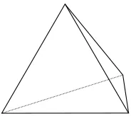
[image:14.612.259.351.525.607.2]

Figure 2: The standard two simplex, ∆2 ⊂R3

(15)

Let X be a topological space. For n _≥ 0 we define the group of singular n-chains in X, Sn(X), to be the free abelian group generated by the set of all continuous maps

σ: ∆n _→ _X_{. For} _{n <} _{0 we define} _S

n(X) = 0. Associating to X the group Sn(X) is

a functor from the category of topological spaces and continuous maps to the category of groups and homomorphisms. The homomorphism f∗: Sn(X) → Sn(Y) associated to

the continuous mapping f: X _→ Y sends σ: ∆n _→ X to f∗σ = f ◦σ: ∆n → Y. This

function from the basis of the free abelian group Sn(X) to Sn(Y) extends uniquely to a

homomorphismSn(X)→Sn(Y).

Our next goal is to provide a boundary map for this construction, so as to define a chain complex, the singular chain complex. As we shall see, to do this it suffices to define an element ∂(∆n) ∈Sn−1(∆n) for each n ≥0. For each index i; 0 ≤i≤n we define the ith-face fi of ∆n. It is an affine linear map fi: ∆n−1 → ∆n determined by the n ordered

points_{v0, v1, . . . , vi−1, vi+1, . . . , vn}. Notice that the image offi is the intersection of ∆n

with the hyperplaneti = 0 inRn+1, and thatfiis an affine isomorphism onto this subspace

preserving the order of the vertices. We define

∂(∆n) =

n

X

i=0

(₋1)ifi ∈Sn−1(∆n).

PSfrag replacements f1 f0

[image:15.612.223.384.325.489.2]

f2

Figure 4: ∂∆2 =f0−f1+f2

More generally, let ζ = P_σnσσ be an element of Sn(X). (Here, our conventions are

that σ ranges over the continuous maps of ∆n to X, the nσ are integers all but finitely

many of which are zero.) Then we define

∂(ζ) =X

σ

nσσ∗(∂(∆n)).

By functorality, the right-hand side of the above equality is naturally an element ofSn−1(X).

Here is the basic lemma that gets this construction going. As we shall see, this will be the first of many similar computations.

Lemma 1.3.1. The composition

Sn+1(X)−→∂ Sn(X)−→∂ Sn−1(X)

(16)

Proof. Clearly, by naturality, it suffices to prove that for all n we have ∂(∂(∆n_{)) = 0}_∈

Sn−2(∆n). For indices 0 ≤ i < j ≤ n let fij: ∆n−2 → ∆n be the affine linear map that

sends ∆n−2 _{isomorphically onto the intersection of ∆}n _{with the codimension-two subspace}

ti=tj= 0 in a manner preserving the ordering of the vertices. We compute:

∂(fi) = n

X

k=i+1

(₋1)k−1fik+ i−1

X

k=0

(₋1)kfki.

Hence,

∂∂(∆n) =

n

X

i=0

(−1)i

n

X

k=i+1

(−1)k−1fik+ i−1

X

k=0

(−1)kfki.

Claim 1.3.2. In this sum, each termfij with 0≤i < j≤nappears exactly twice and with

cancelling signs.

Exercise 1.3.3. Prove this claim.

The content of this lemma is that we have constructed a chain complex, S∗(X). It is called thesingular chain complexof X. It is immediate from what we have already proved and the definitions that this is a functor from the topological category to the category of chain complexes of free abelian groups.

The singular homology of X, denoted H∗(X), is the homology of the singular chain

complex. Singular homology is a functor from the topological category to the category of graded abelian groups and homomorphisms. The group indexed bynis denotedHn(X).

As disscussed in section 1.2.2 above, given a chain complex and an abelian group we can define the homology of the chain complex with coefficents in that abeian group. In particular, let A be an abelian group, then the singular homology of a topological space

X with coefficients in A, denoted H∗(X;A), is by definition the homology of S∗(X)⊗A.

Notice that ifA is a field then these homology groups are vector spaces overA and if A is a ring, then they are modules over A. This is a functor from the category of topological spaces to the category of graded abelian groups (resp., to gradedA-modules).

Likewise, we define the singular cohomology of X with coefficients in A to be the cohomology of the cochain complex S∗₍_X_;_A_{) = Hom(}_S

∗(X), A). A case of particular

interest is whenA=Z. In this case we refer to the cohomology as the singular cohomology ofX.

1.3.2 First Computations

We will now compute some of the singular homology groups of a few spaces directly from the definition.

Lemma 1.3.4. Hi(X) = 0 if i <0.

(17)

Exercise 1.3.5. Show for anyAthat the singular homology with coefficients in Avanishes in dimensions less than zero as does the singular cohomology with values inA.

Since the singular zero chains are what we denoted by S0(X) earlier, and the singular one chains are generated by continuous maps of the interval intoX, and since the boundary of the one chain represented byγ: [0,1]_→ X is γ(1)₋γ(0), it follows that H0(X) is the

quotient of S0(X) by the equivalence relation studied earlier. Hence, we have already established the following result:

Lemma 1.3.6. H0(X) is the free abelian group generated by the set of path components of X.

Exercise 1.3.7. Show that the singular cohomology of a topological space X is ZP(X)_{, the}

group of functions from the set of path components of X to the integers.

1.3.3 The Homology of a Point

Proposition 1.3.8. Let X be a one-point space. Then Hk(X) = 0 for all k 6= 0 and

H0(X) ∼=Z.

Proof. For each n ≥ 0, there is exactly one map of ∆n → X, let us call it σn. Thus,

Sn(X) = Zfor every n≥0. Furthermore, ∂(σn) = Pni=0(−1)iσn−1. This sum is zero if n

is odd and isσn−1 ifnis even and greater than zero. Hence, the group ofn-cycles is trivial

forneven and greater than zero, and is Ker∂n=Zfornodd and forn= 0. On the other

hand, the group ofnboundaries is trivial forneven and all ofSn(X) fornodd. The result

follows immediately.

Exercise 1.3.9. Compute the singular cohomology of a point. For any abelian group A, compute the singular homology and cohomology with coefficients in A for a point.

1.3.4 The Homology of a Contractible Space

We say that a spaceX iscontractibleif there is a pointx0 ∈X and a continuous mapping H: X_×I _→ X with H(x,1) = x and H(x,0) = x0 for all x ∈ X. As an example, Rn is

contractible for all n_≥0.

Exercise 1.3.10. Show Rn _{is contractible.}

Exercise 1.3.11. Show any convex subset Rn _{is contractible.}

Proposition 1.3.12. If X is contractible, then Hi(X) = 0 for all i≥1.

Proof. Let H be a contraction of X to x0. Let σ: ∆k → X be a continuous map. We definec(σ) : ∆k+1 _→X by coning to the origin. Thus,

(18)

One checks easily that this expression makes sense and that ast0→1 the limit exists and

isx0, so that the map is well-defined and continuous on the entire ∆k+1.

Claim 1.3.13. If k_≥1, then ∂(c(σ)) =σ₋Pk_i₌₀(₋1)k_c₍_σ_◦_f i).

This claim remains true for k = 0 if we interpret the cone on the empty set to be the origin.

PSfrag replacements

X

Figure 5: c(σ : ∆1_→X) : ∆2_→X

For all k _≥0, we define c: Sk(X) → Sk+1(X) by c(Pnσσ) = Pnσc(σ). Then claim

1.3.13 implies the following fundamental equation for allζ _∈Sk(X), k ≥1:

∂c(ζ) =ζ₋c(∂ζ) (1)

It follows that if ζ is ak cycle for any k _≥1, then ∂c(ζ) = ζ, and hence the homology class of ζ is trivial. Thus, Hk(X) = 0 for all k > 0. Clearly, we have Hk(X) = 0 for

k <0 and sinceX is path connected, we haveH0(X)∼=Z. This completes the proof of the

proposition.

Exercise 1.3.14. Compute H0(X) for X contractible.

Exercise 1.3.15. For any abelian group A, compute the homology and cohomology of a contractible space with values in A.

1.3.5 Nice Representative One-cycles

Before we begin any serious computations, we would like to give a feeling for the kind of cycles that can be used to represent one-dimensional singular homology. LetX be a path connected space and let a ∈ H1(X) be a homology class. Our object here is to find an especially nice cycle representative fora.

Definition 1.3.16.AcircuitinXis a finite ordered set of singular one simplices{σ1, . . . , σk}

inX with the property thatσi(1) =σi+1(0); for 1≤i≤k−1 andσk(1) =σ1(0).

Given a circuit {σ1, . . . , σk} there is an associated singular one-chain ζ = Pki=1σi ∈

(19)

[image:19.612.261.349.107.217.2]

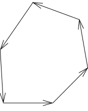
Figure 6: A circuit

Exercise 1.3.17. Show that ζ is a cycle.

Henceζrepresents a homology class [ζ]_∈H1(X). Any such homology class is the image

under a continuous map of a homology class in the circle. To see this, pastek copies of the one-simplex together end-to-end in a circuit to form a circle T, and use the σi, in order,

to define a map ˜ζ: T _→ X. The inclusions of the k unit intervals into T form a singular one-cycle µ ∈S1(T) representing a homology class [µ] ∈H1(T). Clearly, [ζ] = ˜ζ∗[µ]. The

next proposition shows that all elements inH1(X) are so represented, at least whenX is

path connected.

Proposition 1.3.18. Let X be path connected. Given a _∈ H1(X), there is a circuit

{σ1, . . . , σk} such that the singular one-cycleζ =σ1+· · ·+σk represents the class a.

Proof. We sketch the proof and leave the details to the reader as exercises.

Lemma 1.3.19. Every homology class in H1(X) is represented by a cycle all of whose

non-zero coefficients are positive.

Proof. First let us show that we can always find a representative one-cycle such that the only singular one simplices with negative coefficients are constant maps. Givenσ: ∆1→X, written asσ(t0, t1), we form the mapψ: ∆2 →X by ψ(t0, t1, t2) =σ(t0+t2, t1). It is easy

to see that∂∆ =σ+τ₋pwhereτ(t0, t1) =σ(t1, t0) andp(t0, t1) =σ(1,0). We can rewrite

this as an equivalence

−σ ∼=τ ₋p.

Using this relation allows us to remove all negative coefficients from non-trivial singular simplices at the expense of introducing negative coefficients on constant singular one-simplices.

(20)

Corollary 1.3.20. Every homology class in H1(X) is represented by a sum of maps of∆1

toX with coefficients one (but possibly with repetitions).

Now letζ =Pk_i₌₁σi be a cycle. It is possible to choose a subset, such that after possibly

reordering, we have a circuit_{σi1, . . . , σi`}Continuing in this way we can writeζ as a finite sum of singular cycles associated to circuits.

Our next goal is to combine two circuits into a single one (after modifying by a bound-ary). Let ζ and ζ0 _{be cycles associated with circuits} _{_σ

1, . . . , σk} and {σ10, . . . , σ`0}. Since

X is path connected, there is a pathγ: [0,1]→X connectingσ1(0) toσ₁0(0). Then {σ1, . . . , σk, γ, σ10, . . . , σ0`, γ−1}

is a circuit and we claim that its associated cycle is homologous to the sum of the cycles associated to the two circuits individually. (Here,γ−1₍_t

[image:20.612.188.422.289.507.2]

0, t1) =γ(t1, t0).)

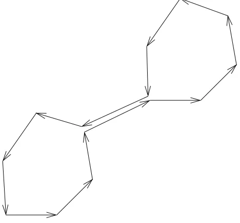
Figure 7: Joining two circuits together

Exercise 1.3.21. Prove this last statement.

An inductive argument based on this construction then completes the proof of the proposition.

1.3.6 The First Homology of S1

(21)

Theorem 1.3.22.

H1(S1)∼=Z.

The proof of this result is based on the idea of winding numbers.

Claim 1.3.23. Let I be the unit interval, and let f: I → S1 be a continuous mapping. Then there is a continuous function θ: I _→ R such that for all t _∈ I exp(iθ(t)) = f(t). The function θ is unique up to adding a constant integral multiple of 2π. In particular,

θ(1)−θ(0) is independent of θ. This difference is called the winding numberwinding numberwinding number w(f) of f. Furthermore, exp(iw(f)) =f(1)f(0)−1.

Proof. Let us consider uniqueness first. Suppose that θ and θ0 are functions as in the claim. Then exp(iθ(t)) = exp(iθ0₍_t_{)) for all} _t_∈_I_{. Hence,}_θ₍_t₎₋_θ0₍_t_{) is an integral multiple}

of 2π. By continuity, this multiple is constant as we vary t.

Now we turn to existence. We consider the set _S = _{t _∈ I_} for which a function

θ as required exists for the subinterval [0, t]. Clearly, 0 _{∈ S}. Suppose that t _{∈ S}, and let θ0: [0, t] → R be as required. There exists an open subset U ⊂ I containing t such

that f(U) _⊂ S1 _{\ {−}f(t)_} =: T. There is a continuous function θT: T → R such that

exp(iθT(x)) = x for all x ∈ T. By adding an integral multiple of 2π we can assume that

θT(f(t)) = θ0(t). Defining θ0 to be θ on [0, t] and to be θT ◦f on U gives a function as

required on [0, t]_∪U. This shows that _S is an open subset of I. To show that _S is closed suppose that we have a sequence tn → t and functions θn: [0, tn] → R as required. By

adjusting by integral multiples of 2π we can arrange that all these functions take the same value at 0. Then by uniqueness, we see that θn and θm agree on their common domain

of definition. Thus together they define a function of _∪∞

n=1[0, tn] which surely includes

[0, t). It is easy to see that the limit as n 7→ ∞ of θ(tn) exists and hence can be used to

extend the map to a continuous map on [0, t], as required. To see this, look at an interval

U _⊂S1 _containing_f₍_t_{). Now, consider the preimage of}_U _in_R_{under the exponential map} x7→expix. This is a disjoint union of intervals, qUi mapping homeomorphically to U, and

we have θ((t₋, t))_⊂Ui for some i. Now, it should be clear that the limit exists, and we

define θ(t) = lim

tn→t

θ(tn). Since S is open and closed and contains 0, it follows that S =I

and hence 1_{∈ S}, which proves the result.

In fact the argument above can be used to show the following

Corollary 1.3.24. Suppose that f, g are close maps of I toS1, close in the sense that the angle between f(t) and g(t) is uniformly small. Then there are functions θf and θg from

I _→Ras above which are close, and in particular w(f) and w(g) are close.

For a singular 0-chainµ=P_pnppinS1, we defineθ(µ) =Q_ppnp, using the

multiplica-tive group structure ofS1.

Lemma 1.3.25.Letζ =Pk_i₌₁niσibe a singular one-chain inS1. Definew(ζ) =Pk_i₌₁niw(σi).

(22)

Proof. By the multicative property of both sides, it suffices to prove this equality for a singular one-simplex, where it is clear.

Corollary 1.3.26. If ζ is a singular one-cycle inS1_{, then} _w₍_ζ₎_∈₂_π_Z_.

We define a function from the abelian group of one cycles to Z by associating to a cycle ζ the integer w(ζ)/2π. This function is clearly additive and hence determines a homomorphismw from the group of one-cycles toZ.

Claim 1.3.27. If ζ is a boundary, then w(ζ) = 0.

Proof. Again by multiplicativity, it suffices to show that ifζ=∂τ whereτ: ∆2 →S1 is a singular two simplex, then w(ζ) = 0. To establish this we show that there is a continuous function θ: ∆2 _→ _R _{such that exp(}_iθ₍_x_{)) =} _τ₍_x_{) for all} _x _∈ _∆2_{. First pick a lifting} θ(1,0,0) ∈Rfor τ(1,0,0) ∈S1. Now for each (a, b) with a, b≥0 and a+b= 1, consider the interval_{t0,(1−t0)a,(1−t0)b}. There is a unique liftingθa,bmapping this interval into

R lifting the restriction of τ to this interval and having the given value at (1,0,0). The continuity property described above implies that these lifts fit together to give the map

θ: ∆2 →R as required. Once we have this map we see that w(f0) = θ(0,0,1)−θ(0,1,0), w(f1) =θ(0,0,1)−θ(1,0,0) andw(f2) =θ(0,1,0)−θ(1,0,0), so thatw(f0)−w(f1)+w(f2) =

0.

Exercise 1.3.28. Prove that the map θ constructed above is continuous.

It now follows that we have a homomorphismW: H1(S1)→Z. We shall show that this

map is an isomorphism. The mapI _→S1_{given by}_t_7→_exp(2_πit_{) is a one cycle whose image}

underwis 1. This proves thatW is onto. It remains to show that it is one-to-one. Suppose that ζ is a cycle and w(ζ) = 0. According to proposition 1.3.18, we may as well assume thatζ is the cycle associated to a circuit_{σ1, . . . , σk}. We choose liftings ˜σ`: I →R with

exp(iσ˜`(t)) = σ`(t) for all ` and all t∈ I. We do this in such a way that ˜σ`+1(0) =σ`(1)

for 1_≤` < k. The difference ˜σk(1)−σ˜1(0) is 2πw(ζ), which by assumption is zero. This

implies that the circuit inS1 lifts to a circuit inR. Let ˜ζ be the one cycle in Rassociated to this circuit. By Proposition 1.3.12 there is a two-chain ˜µinRwith∂µ˜ = ˜ζ. Let µbe the two-chain inS1 that is the image of ˜µunder the exponential mapping. We have ∂(µ) =ζ, and hence that ζ represents the trivial element in homology. This completes the proof of the computation ofH1(S1).

Exercise 1.3.29. Complete the proof of Corollary 1.3.20

Exercise 1.3.30. State and prove the generalization of Proposition 1.3.18 in the case of a general spaceX.

(23)

Exercise 1.3.32. Show that if X is path connected then for any a _∈ H1(X), there is a

map f: S1 →X and an element b∈H1(S1) such that a=f∗(b).

Exercise 1.3.33. Let X be path connected and simply connected (which means that every continuous map ofS1 _→X extends over D2). Show that H1(X) = 0.

1.4 An Application: The Brouwer Fixed Point Theorem

As an application we now prove a famous result. Recall that aretractionof a spaceX onto a subspaceY _⊂X is a continuous surjective mapϕ:X _→Y such thatϕ_|Y = IdY.

Theorem 1.4.1. There is no continuous retraction of the2-disk D2 onto its boundary S1.

Proof. Leti: S1 _→D2be the inclusion ofS1as the boundary ofD2. Suppose a continuous retractionϕ:D2_→_S1 _{of the disk onto its boundary exists. Then the composition}

S1 _−→i D2 _−→ϕ S1,

is the identity. Since homology is a functor we have

H1(S1) i

∗

−→H1(D2) ϕ

∗

−→H1(S1)

is the identity. But sinceH1(D2) = 0 since the disk is contractible, and H1(S1)6= 0, this

is impossible. Hence, no suchϕexists.

This leads to an even more famous result.

Theorem 1.4.2. The Brouwer Fixed Point TheoremAny continuous map of the two disk, D2, to itself has a fixed point.

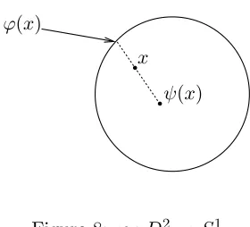
Proof. Suppose that ψ: D2 → D2 is a continuous map without a fixed point. Then, the pointsxand ψ(x) are distinct points of the disk. The lineL(x) passing through xand

ψ(x) meets the boundary of the diskS1 _{in two points. Let} _ϕ₍_x_{) be the point of} _L₍_x₎_∩_S1

that lies on the open half-ray of this line beginning at ψ(x) and containing x. One sees easily that L(x) and ϕ(x) vary continuously with x. Thus, ϕ(x) is a continous mapping

D2 _→ _S1_{. Also, it is clear that if} _x _∈_S1_{, then}_ϕ₍_x_{) =}_x_{. This contradicts theorem 1.4.1}

and concludes the proof of the Brouwer fixed point theorem.

Exercise 1.4.3. Show that ϕ is continuous.

(24)

PSfrag replacements

ϕ(x)

ψ(x)

[image:24.612.234.374.100.227.2]

x

Figure 8: ϕ:D2 _→S1

2 The Axioms for Singular Homology and Some Consequences

As the above computations should indicate, it is quite difficult to compute singular homol-ogy directly from the definition. Rather, one proceeds by finding general properties that homology satisfies that allow one to compute homology for a large class of spaces from a sufficiently detailed topological description of the space. These general properties are called theaxioms for homology. One can view this in two ways – from one point of view it is a computational tool that allows one to get answers. From a more theoretical point of view, it says that any homology theory that satisfies these axioms agrees with singular homology, no matter how it is defined, at least on the large class of spaces under discussion.

2.1 The Homotopy Axiom for Singular Homology

The result in section 1.3.4 that the homology groups of a contractible space are the same as those of a point has a vast generalization, theHomotopy Axiomfor homology.

Definition 2.1.1. Let X and Y be topological spaces. We say two maps f, g: X → Y

are homotopic if there is a continuous map F: X _×I _→ Y with F(x,0) = f(x) and

F(x,1) =g(x) for allx_∈X. The map F is called a homotopyfromf to g.

Lemma 2.1.2. Homotopy is an equivalence relation on the set of maps from X to Y.

Exercise 2.1.3. Prove this lemma.

(25)

f0_{. Then the map}_H0 ₌_g_◦_H_:_X_×_I _→_Z _{is continuous since both}_H _and_g_{are continuous}

and we have H0(x,0) = g◦H(x,0) = g◦f and H0(x,1) = g◦H(x,1) = g◦f0. So H0

is a homotpy from g_◦f to g_◦f0_{, and thus [}_g_◦_f_{] = [}_g_◦_f0_{]. A similar argument shows}

that the defintion is independent of the representative we choose for [g]. For any object

X of HomotopyHomotopyHomotopy, we have the identity morphism, [IdX] : X → X is just the hompotopy

class represented by the identity map on X. Similarly, the morphisms in this category are associative under composition because the underlying representatives of the homotopy classes are associative. Notice that in the category HomotopyHomotopyHomotopy, it doesn’t make sense to ask for the value of a morphism at a point in X. Unlike the morphisms in many other categories we have seen, such as the algebraic categories of groups or rings, there is no specific set function underlying a morphism in this category. Also, notice that there is a natural functor from the category T opT opT op of topological spaces and continuous maps to the categoryHomotopyHomotopyHomotopy given by sending a topological space to itself and sending a continuous function to the homotopy class represented by that function.

We say that a map f: X _→ Y is a homotopy equivalence if there is a map g: Y _→ X

such thatg_◦f is homotopic to IdX andf ◦gis homotopic to IdY. Show that the relation

X is homotopy equivalent toY is an equivalence relation.

Recall, (See A) in any category _C a morphism f : a _→ b is called an isomorphism if there is another morphismf0 _:_b_→_a _in_C _{such that} _f0_◦_f _{= Id}

a and f◦f0 = Idb. If such

a morphismf0 exists, it is unique and we write f0 =f−1. Two objects aand b are said to beisomorphic if there exists an isomorphism between them.

Exercise 2.1.4. What are the isomorphisms in the category HomotopyHomotopyHomotopy?

Lemma 2.1.5. Let X be a space and x0 ∈X a point. Then the inclusion of x0 into X is

a homotopy equivalence if and only if X is contractible to x0.

Exercise 2.1.6. Prove this lemma.

Now we are ready to state the vast generalization alluded to above.

Theorem 2.1.7. The Homotopy Axiom for Singular Homology Let X and Y be topological spaces and let f, g: X _→Y. If f andg are homotopic, then f∗=g∗: H∗(X)→ H∗(Y).

The Homotopy Axiom is most frequently used in the form of the following immediate corollary.

Corollary 2.1.8. If f: X → Y is a homotopy equivalence, then f∗: Hn(X) → Hn(Y) is

an isomorphism for every n.

In the language of categories, this corollary to the homotopy axiom says that the singular homology functor from the category of topological spaces to the category of graded abelian groups factors through the natural functor fromT opT opT optoHomotopyHomotopyHomotopy.

(26)

Definition 2.1.9. LetC∗ and D∗ be chain complexes andf∗, g∗: C∗ →D∗ be morphisms

in the category of chain complexes. A chain homotopy from f∗ to g∗ is a collection of

homomorphisms, one for each integer k, Hk: Ck→Dk+1 satisfying

∂_◦Hk+Hk−1◦∂=g∗−f∗.

Claim 2.1.10. Chain homotopy is an equivalance relation on morphisms from C∗ to D∗.

Exercise 2.1.11. Prove this claim.

Claim 2.1.12. If f∗, g∗: C∗ →D∗ are chain homotopic, then the maps that they induce on

homology are equal.

Proof. Ifζ _∈Ck is a cycle, then,

∂(Hk(ζ)) =g∗(ζ)−f∗(ζ).

Thus, in order to prove the Homotopy Axiom it is sufficent to prove the following proposition:

Proposition 2.1.13. Iff, g: X _→Y are homotopic, thenf∗, g∗: S∗(X)→S∗(Y)are chain

homotopic.

Proof. Since ∆k_×_I _{is a product of affine spaces and hence is itself affine, we can define}

an affine map of a simplex ∆n into it by simply giving an ordered set of n+ 1 points in the space. We denote the affine map of ∆n into ∆k_×I determined by (x0, . . . , xn) by this

orderedn+ 1-tuple. We denote byui the point (vi,0) in ∆k×I and bywi the point (vi,1).

LetH(∆k)∈Sk+1(∆k×I) be defined by

H(∆k) =

k

X

i=0

(₋1)i(u0, . . . , ui, wi, . . . , wk).

Claim 2.1.14.

∂(H(∆k)) = ∆k_{× {}1_{} −}∆k_{× {}0_{} −}

k

X

i=0

(₋1)k(fi×IdI)∗(H(∆k−1)).

Proof.

(27)

k

X

i=0

(₋1)i _Xi

j=0

(₋1)j(u0, . . . ,uˆj, . . . , ui, wi, . . . , wk) + k

X

j=i

(₋1)j+1(u0, . . . , ui, wi, . . . ,wˆj, . . . , wk)

= X

j<i

(₋1)i+j(u0, . . . ,uˆj, . . . , ui, wi, . . . , wk) +

X

j>i

(₋1)i+j+1(u0, . . . , ui, wi, . . . ,wˆj, . . . , wk)+

k

X

i=0

(u0, . . . , ui−1, wi, . . . , wk)−(u0, . . . , ui, wi+1, . . . , wk).

The last term telescopes to leave only,

(w0, . . . , wk)−(u0, . . . , uk) = ∆k× {1} −∆k× {0},

and so we obtain,

∂(H(∆k)) =X

j<i

(₋1)i+j(u0, . . . ,uˆj, . . . , ui, wi, . . . , wk) (2)

+X

j>i

(−1)i+j+1(u0, . . . , ui, wi, . . . ,wˆj, . . . , wk)

+ ∆k_{× {}1_{} −}∆k_{× {}0_}.

Now consider ∆k−1 _×I. Let x0, . . . , xn−1 denote the vertices at 0, and y0, . . . , yn−1

denote the vertices at 1. Then,

(fj×IdI)(xj) =

(

ui j > i

ui+1 j 6i

(fj×IdI)(yj) =

(

wi j > i

wi+1 j6i

Now, we consider H(∂∆k_{). It is defined to be,} k

X

j=0

(₋1)j(fj ×IdI)(H(∆k−1) = k

X

j=0

(₋1)j(fj×IdI)( k−1

X

i=0

(₋1)i(x0, . . . , xi, yi, . . . , yk)) =

k

X

j=0

(−1)j _Xj−1

i=0

(−1)i(u0, . . . , ui, wi, . . . ,wˆj, . . . , wk) + j−1

X

i=0

(−1)i−1(u0, . . . ,uˆj, wi+1, . . . , . . . , wk)

= X

j>i

(₋1)i+j(u0, . . . , ui, wi, . . . ,wˆj, . . . , wk) +

X

j<i

(₋1)i+j−1(u0, . . . ,uˆj, . . . , ui, wi, . . . , wk) =

− X

j>i

(−1)i+j+1(u0, . . . , ui, wi, . . . ,wˆj, . . . , wk) +

X

j<i

(−1)i+j(u0, . . . ,uˆj, . . . , ui, wi, . . . , wk)

(28)

Comparing to the formula (2) we found above for∂(H(∆k_{)), we see that we have,}

∂(H(∆k)) = ∆k× {1} −∆k× {0} −

k

X

i=0

(−1)k(fi×IdI)∗(H(∆k−1)).

Suppose thatF: X×I→Y is a homotopy fromf tog. Then we defineF∗:Sk(X)→

Sk+1 by

F∗(σ) =F ◦(σ×IdI)∗(H(∆k)).

Claim 2.1.15. F∗ is a chain homotopy from f∗ to g∗.

Proof.

∂F∗(σ) = (F ◦(σ×IdI)∗(∆k× {1} −∆k× {0} −H(∂∆k)) =g∗(σ)−f∗(σ)−F∗(∂σ).

So,

∂F∗(σ) +F∗(σ) =g∗(σ)−f∗(σ),

and thusF∗ is a chain homotopy fromf to g.

The proposition now follows immediately.

This completes the proof of the homotopy axiom. In brief, these were the main steps: Step 1. Chain homotopic maps induce the same map on homology.

Step 2. Define an element H(∆k)∈Sk+1(∆k×I) with the property

∂(H(∆k)) = ∆k_{× {}1_{} −}∆k_{× {}0_{} −}

k

X

i=0

(₋1)k(fi×IdI)∗(H(∆k−1)).

Step 3. Given a homotopy F fromf to g useH(∆k_{) to define a chain homotopy}_F

∗ from f∗ to g∗ by

(29)

2.2 The Mayer-Vietoris Theorem for Singular Homology

The next axiom is a result that allows us to compute the homology of a union of two open sets provided that we know the homology of the sets themselves and the homology of their intersection.

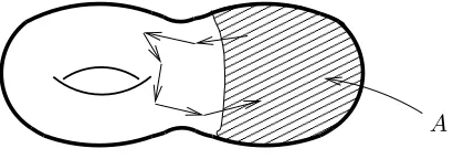
Theorem 2.2.1. LetX be a topological space andU, V open subsets ofX so thatX =U_∪V. LetjU: U ,→X andjV: V ,→X andiU: U∩V ,→U andiV: U∩V ,→V be the inclusions.

Then there is a long exact sequence of homology groups:

· · · →Hk(U ∩V)

(iU)∗−(iV)∗

−−−−−−−−→ Hk(U)⊕Hk(V)

(jU)∗+(jV)∗

−−−−−−−−→ Hk(X) −−−−→ Hk−1(U ∩V)→ · · ·

In order to prove this we will need the following homological lemma: Lemma 2.2.2. Suppose we have a short exact sequence of chain complexes:

0 _{−−−−→} A∗ f

∗

−−−−→ B∗ g

∗

−−−−→ C∗ −−−−→ 0;

that is, we have three chain complexes, A∗, B∗, C∗ with chain complex morphisms f∗ : A∗ →B∗ and g∗ :B∗→C∗ such that for every n we have a short exact sequence:

0 −−−−→ An −−−−→fn Bn −−−−→gn Cn −−−−→ 0

Then there exists a connecting homomorphism β :Hk(C∗)→Hk−1(A∗) making the

follow-ing long exact sequence in homology:

· · · −−−−→ Hn(A∗) f

∗

−−−−→ Hn(B∗) g

∗

−−−−→ Hn(C∗) −−−−→β Hn−1(A∗) −−−−→ · · ·

Proof. The proof is an exercise in what is known as diagram chasing. Diagram chasing is very common in algebraic topology, but it is a technique that is extremely tedious to read and only becomes comfortable with practice. We will write out explicitly the begining of the proof and leave the rest to the reader. To begin we will prove exactness at Hn(B∗).

Exactness at this point involves only the maps on homology induced by f∗ and g∗, not

the connecting homomorphism. First, we have g∗◦f∗ = 0 holds on the chain level, so it is also true on homology. Now, let [ζ] _∈ Hn(B∗). Suppose that g∗[ζ] = 0. This implies g∗(ζ) = ∂cn+1 for some cn+1 ∈Cn+1. By exactness at Cn+1, there is a bn+1 ∈ Bn+1 that

maps to cn+1 under gn+1. Let ζ0 = ζ−∂bn+1. Then ζ0 is clearly a cycle, and [ζ] = [ζ0].

Applyingg∗ we see that

g∗(ζ0) =g∗(ζ)−g∗(∂bn+1) =g∗(ζ)−∂(f∗(bn+1)) =g∗(ζ)−g∗(ζ) = 0

as a chain, so exactness implies there exists anan∈An so thatf∗(an) =ζ0. Now, we need

to show ∂(an) = 0. We have ∂ζ0 = 0 and therefore, by commutativity, f∗(∂(an)) = 0, but

(30)

Construction of the connecting homomorphism, β, makes use of the following commu-tative diagram:

0 _{−−−−→} An+1

fn+1

−−−−→ Bn+1

gn+1

−−−−→ Cn+1 −−−−→ 0

  y   y   y

0 _{−−−−→} An fn

−−−−→ Bn gn

−−−−→ Cn −−−−→ 0

  y   y   y

0 _{−−−−→} An−1

fn−1

−−−−→ Bn−1

gn−1

−−−−→ Cn−1 −−−−→ 0

  y   y

0 −−−−→ An−2

fn−1

−−−−→ Bn−2

Start with a homology class [c] _∈ Hn(C∗) represented by a cycle c∈Cn. By exactness at

Cn there is a bn ∈ Bn so that gn(bn) = c. By comutativity of the diagram gn−1(∂bn) =

∂gn(bn) =∂c= 0, sincecis a cycle. Then by exactness at Bn−1, since bn−1∈Ker(gn−1) =

Im(fn−1) there is an elementan−1 ∈An−1 so thatfn−1(an−1) =∂bn. We need to show that

an−1 is a cycle. By commutativity of the diagramfn−2(∂an−1) =∂fn(an−1) =∂∂bn−1 = 0.

Then by exactness atAn−1, fn−1 is an injection, so∂an−1 = 0. Thus,an−1 is a cycle.

We made a choice when we picked a bn in the pre-image of c. If we choose another

element b0

n so that gn(b0n) =c, we have gn(b0n−bn) = gn(b0n)−gn(bn) = c−c= 0. That

is, bn and b0n differ by an element in the Kergn =Imfn. So we have b0n = bn+fn(an) for

some an ∈An. Following this through our construction, we see that this changes an−1 to an−1+∂an, and thus does not change our map on homology.

Now, suppose we choose a different cycle representative for [c], say c+∂c0_n₊₁ for some

c0_n₊₁ _∈ Cn+1. Then, by exactness at Cn+1 there is an element b0n+1 ∈ Bn+1 so that gn+1(b0n=1) = cn0+1. Then a natural choice for an element in Bn that maps to c+∂c0n+1

under gn is b+∂bn0+1. Notice we can choose any element in the pre-image of c+∂c0n+1

that we want, since we have already shown that our construction is independent of this choice. But now, if we continue with our construction, we see that we get the same element

an−1 ∈An−1 as before. So, we have a well defined map β : Hn(C∗) →Hn−1(A∗) given by

[c]7→[an−1]. We leave the proof of exactness at H∗(A∗) andH∗(C∗) as an exercise.

Now that we have proven this lemma, we need to find an appropriate short exact sequence of chain complexes that will give rise to the Mayer-Vietoris sequence in homology. At first glance, the most likely candidate would be:

0 _{−−−−→} S∗(U ∩V)

(iU)∗−(iV)∗

−−−−−−−−→ S∗(U)⊕S∗(V)

(jU)∗+(jV)∗

−−−−−−−−→ S∗(X) −−−−→ 0

(31)

X that do not come from the inclusions of singular chains in U and singular chains in V, those chains that have maps σ : ∆n → X with neither Im(σ) * U nor Im(σ) * V. To force exactness at this point we replace S∗(X) with the subcomplex S∗small(X) generated

by the singular simplices whose images lie in either U orV. We call these chains, and the simplices of which they are madesmall. Then one can easily check that

0 _{−−−−→} S∗(U ∩V)

(iU)∗−(iV)∗

−−−−−−−−→ S∗(U)⊕S∗(V)

(jU)∗+(jV)∗

−−−−−−−−→ Ssmall

∗ (X) −−−−→ 0

is a short exact sequence of chain complexes. By our homolgical lemma, this induces a long exact sequence in homology:

· · · →Hn(U ∩V)→Hn(U)⊕Hn(V)→Hn(S∗small(X))→Hn−1(U∩V)→ · · ·

Now, we need to show that in fact, the inclusion Ssmall

∗ (X) ,→ S∗(X) induces an

iso-morphism on homology. To do this we will define the subdivision map sd:S∗(X)→S∗(X)

and a chain homotopy from this map to the identity, showing that it induces the identity on homology.

First we will define a map sd, which given ann-simplex ∆n, assigns a chain inSn(∆n).

In order to define this map it will be convinient to think of then-simplex in three equivalent ways. We can write then-simplex as a sequence of inclusions of faces ∆n₌_τ0_⊂_τ1 _{⊂ · · · ⊂} τn, whereτi is ani-face of ∆n. There are exactly (n+ 1)! ways of doing this corresponding to the (n+ 1)! elements of the permutation group Σn+1 of the n+ 1 vertices of ∆n. To

see this, we give a correspondance between ordered lists of the n+ 1 vertices, and the expression of ∆n as a sequence of inclusions of faces. Given an ordered list of the vertices (v0, v1, . . . , vn) we let τi be the face of ∆n with vertices v0, v1, . . . , vi. Given a sequence of

faces, ∆n ₌_τ0 _⊂ _τ1 _{⊂ · · · ⊂} _τn_{, we obtain an ordered list of vertices by letting} _v

0 = τ0, v1 the vertex of τ1 not in τ0 and so on. Then given a permutation p∈Σn+1, we have the

sequence of faces corresponding to the ordered list of vertices (vp(0), vp(1), . . . , vp(n)). So we

have the following three ways of thinking of then-simplex:

Σn+1 ⇔ {ordered lists of vertices} ⇔ {sequences of inclusions of faces}

For a faceτiof ann-simplex define ˆτito be the image underτiof (1/(i+1), . . . ,1/(i+1)).

The point ˆτi _{is called the} _barycenter _of _τi_{. Then, given a sequence of inclusions of faces}

τ0⊂τ1⊂ · · ·τn, we obtain a map of then-simplex into itself given by the inclusion of the

n-simplex with vertices the barycenters of the faces:

τ0 ⊂τ1 ⊂ · · · ⊂τn (ˆτ0, . . . ,τˆn) : ∆n,→∆n Now we define sd(∆n₎_∈_S

n(∆n) by

sd(∆n) = X

τ0_⊂_τ1_⊂···⊂_τn

(−1)|p|(ˆτ0,τˆ1, . . . ,τˆn)

(32)

PSfrag replacements

v1 v2

v0

(01) (20)

(120) (021)

(12)

[image:32.612.236.393.102.262.2]

∅

Figure 9: sd(∆2)

Now, forζ _∈Sn(X) whereζ =Paσ(σ: ∆n→X) we define sd(ζ) =Paσσ∗(sd(∆n))∈ Sn(X). We need to show that sd: S∗(X) → S∗(X) is a chain complex morphism. By

naturality, it is sufficent to prove the following lemma. Lemma 2.2.3. ∂sd(∆n) = sd(∂∆n)

Proof. We have,

∂sd(∆n) =∂ X

τ0_⊂···⊂_τn

(₋1)|p|(ˆτ0,τˆ1, . . . ,τˆn)

= X

τ0_⊂···⊂_τn

(₋1)|p|∂(ˆτ0,τˆ1, . . . ,τˆn) =

X

τ0_⊂···⊂_τn (−1)p

_Xn

i=0

(−1)i(ˆτ0,τˆ1, . . . ,τˆi−1,τˆi+1, . . . ,τˆn)

Supposei6= n, and τ0 ⊂ · · · ⊂ τi−1 ⊂τi+1 ⊂. . .⊂ τn is a chain. Then, in passing from

τi−1toτi+1we add two verticesw, w0. Hence, there are exactly twoi₋simplices that we can insert at this point in the chain to form a complete chain, the corresponding permutations differ by a two-cycle interchangingw and w0, and hence have opposite signs. So, all of the terms withi < n cancel in pairs and we are left with

∂sd(∆n) = X

τ0_⊂···⊂_τn

(₋1)|p|(₋1)n(ˆτ0,τˆ1, . . . ,ˆτn−1)

We can write this as,

X

τ0_⊂···⊂_τn

(−1)|p|(−1)n(ˆτ0,τˆ1, . . . ,τˆn−1) =

n

X

j=0

_X

{permutations p|p(n)=j}