Maximum Allowable Load On Wheeled Mobile Manipulators (RESEARCH NOTE)

RESEARCH NOTE

MAXIMUM ALLOWABLE LOAD ON WHEELED MOBILE

MANIPULATORS

M. Habibnejad Korayem and H. Ghariblu

Department of Mechanical Engineering, Iran University of Science and Technology Tehran, Iran, hkorayem@iust.ac.ir

(Received: February 9, 2002 – Accepted in Revised Form: May 15, 2003)

Abstract This paper develops a computational technique for finding the maximum allowable load

of mobile manipulators for a given trajectory. The maximum allowable loads which can be achieved by a mobile manipulator during a given trajectory are limited by the number of factors; probably the dynamic properties of mobile base and mounted manipulator, their actuator limitations and additional constraints applied to resolving the redundancy are the most important factors. To resolve extra D.O.F introduced by the base mobility, additional constraint functions are proposed directly in the task space of mobile manipulator. Finally, in two numerical examples involving a two-link planar manipulator mounted on a differentially driven mobile base, application of the method to determining maximum allowable load is verified. The simulation results demonstrates the maximum allowable load on a desired trajectory has not a unique value and directly depends on the additional constraint functions which applies to resolve the motion redundancy.

Key Words Given Trajectory, Load Carrying Capacity, Base Replacement, Manipulator

ﻩﺪﻴﮑﭼ

ﻩﺪﻴﮑﭼ

ﻩﺪﻴﮑﭼ

ﻩﺪﻴﮑﭼ

ﺮﻴﺴﻣﻚﻳﺭﺩﺭﺍﺩﺥﺮﭼﻲﺗﺎﺑﺭ ﻱﺎﻫﻭﺯﺎﺑﺭﺎﺑﻞﻤﺣﺖﻴﻓﺮﻇﺮﺜﻛﺍﺪﺣﻦﻴﻴﻌﺗﻲﺗﺎﺒﺳﺎﺤﻣﺵﻭﺭﻪﻟﺎﻘﻣﻦﻳﺍﺭﺩ

ﺪﻳﺁﻲﻣ ﺖﺳﺪﺑﺺﺨﺸﻣ

. ﺮﻴﺴﻣ ﻲﺣﺍﺮﻃﺭﺩ ﻢﻬﻣ ﻱﺎﻫﺭﺎﻴﻌﻣﺯﺍ ﻲﻜﻳﻞﻤﺣ ﻞﺑﺎﻗﺭﺎﺑ ﺮﺜﻛﺍﺪﺣﺎﺑ ﻭﺯﺎﺑﻚﻳ ﺖﻛﺮﺣ

ﻲﻣﺖﻛﺮﺣ

ﺪﺷﺎﺑ .

ﺍﺭﻙﺮﺤﺘﻣﻲﺗﺎﺑﺭﻱﻭﺯﺎﺑﻚﻳﺭﺎﺑﻞﻤﺣﺖﻴﻓﺮﻇﺪﻨﻧﺍﻮﺗﻲﻣﻱﺩﺪﻌﺘﻣﻞﻣﺍﻮﻋ ﺪﻨﻫﺩﺭﺍﺮﻗﺮﻴﺛﺄﺗﺖﺤﺗ

.

ﻪﻠﺌﺴﻣ ﻞﺣ ﻱﺍﺮﺑ ﻪﻛ ﻲﻓﺎﺿﺍ ﻱﺎﻫﺪﻴﻗ ﻭ ﻙﺮﺤﺘﻣ ﻱﺎﻫﺭﻮﺗﻮﻣ ﺭﻭﺎﺘﺸﮔ ﺖﻳﺩﻭﺪﺤﻣ ،ﻭﺯﺎﺑ ﻭ ﻪﻳﺎﭘ ﻲﻜﻴﻣﺎﻨﻳﺩ ﺹﺍﻮﺧ

ﺪﻧﺩﺮﮔﻲﻣ ﻝﺎﻤﻋﺍ ﺩﺍﺯﺎﻣ ﻱﺩﺍﺯﺁ ﺕﺎﺟﺭﺩ

, ﻲﻣ ﻲﻘﻠﺗﻢﺘﺴﻴﺳ ﺭﺎﺑ ﻞﻤﺣ ﺖﻴﻓﺮﻇ ﺭﺩ ﺭﺍﺬﮔ ﺮﻴﺛﺄﺗ ﻞﻣﺍﻮﻋ ﻦﻳﺮﺘﻤﻬﻣ ﺯﺍ

ﺪﻧﺩﺮﮔ .

ﻛﺮﺣ ﻪﻄﺳﺍﻮﺑﻪﻛﻲﻓﺎﺿﺍ ﺩﺍﺯﺎﻣ ﺕﺎﺟﺭﺩﻪﻠﺌﺴﻣﻞﺣﻱﺍﺮﺑ

ﻪﺑﻲﻳﺎﻫﺪﻴﻗ،ﺪﻧﺩﺮﮔ ﻲﻣﻞﻴﻠﺤﺗﻢﺘﺴﻴﺳ ﻪﺑﻪﻳﺎﭘ ﺖ

ﺪﻧﺍﻩﺪﺷﻩﺩﻭﺰﻓﺍﻢﺘﺴﻴﺳﺖﻛﺮﺣﻪﻟﺩﺎﻌﻣﻪﺑﻊﺑﺍﻮﺗﺕﺭﻮﺻ .

ﻱﺩﺪﻋﻝﺎﺜﻣﻪﻧﻮﻤﻧﻭﺩﺭﺩ ,

ﻱﺍﻪﺤﻔﺻﻲﻜﻨﻴﻟﻭﺩﻱﻭﺯﺎﺑﻚﻳ

ﻩﺩﺎﻔﺘﺳﺍﺭﺎﺑﻞﻤﺣﺖﻴﻓﺮﻇﻦﻴﻴﻌﺗﺵﻭﺭﺩﺮﺑﺭﺎﻛﺶﻳﺎﻤﻧﻱﺍﺮﺑ،ﺖﺳﺍﻩﺪﺷﺐﺼﻧﺭﺍﺩﺥﺮﭼﻙﺮﺤﺘﻣﻪﻳﺎﭘﻚﻳﻱﻭﺭﻪﻛ

ﺗﺩﺭﻮﻣﻢﺘﻳﺭﻮﮕﻟﺍﺖﺤﺻﻭﻩﺪﺷ

ﺖﺳﺍﻪﺘﻓﺮﮔﺭﺍﺮﻗﻖﻴﻘﺤ .

ﺭﺎﺑﺮﺜﻛﺍﺪﺣﻪﻛﺪﻫﺩﻲﻣﻥﺎﺸﻧﺡﻮﺿﻮﺑﻱﺯﺎﺳﻪﻴﺒﺷﺞﻳﺎﺘﻧ

ﻲﻣﻝﺎﻤﻋﺍﺩﺍﺯﺁﻪﺟﺭﺩﻪﻠﺌﺴﻣ ﻞﺣﻱﺍﺮﺑﻪﻛﺖﺳﺍ ﻲﻳﺎﻫﺪﻴﻗﻉﻮﻧﺯﺍﻲﻌﺑﺎﺗ ﺺﺨﺸﻣﺮﻴﺴﻣﻚﻳ ﺭﺩﻞﻤﺣﻞﺑﺎﻗﺯﺎﺠﻣ ﺩﺭﺍﺪﻧﻲﻳﺎﺘﻜﻳﺭﺍﺪﻘﻣﻭﺩﺩﺮﮔ .

1. INTRODUCTION

The maximum allowable load of a fixed base manipulator is often defined as the maximum payload that the manipulator can repeatedly lift in its fully extended configuration. However, to determine the maximum allowable load of a robot must take into account the inertia effect of the load along a desired trajectory as well as the manipulator dynamics. Wang and Ravani were shown the maximum allowable load of a fixed base manipulator on a given trajectory is primarily

Papadopoulos and Gonthier considered the effect of base mobility of robotic manipulators on large force quasi-static tasks [6]. They introduced the force workspace concept for identifying proper base guaranteeing task execution along desired paths. In their work the dynamic effects of the load and manipulator are not examined. There are some other works, which published about carrying heavy loads and stability of the wheeled mobile manipulators [7-9]. Also there are some other research studies which consider the problem of large force task planning and carrying heavy loads on mobile manipulators, however non of them consider the problem of finding maximum load carrying capacity of mobile manipulators.

In this paper, we present a new method of determining the maximum allowable load for mobile manipulators subject to both actuator and redundancy constraints. For motion planning and redundancy resolution, additional constraint functions and the augmented Jacobian matrix are used. The recursive Newton-Euler method is used to formulate the dynamic effects of combined mobile base and manipulator motion on joint actuator torques. A general computational procedure is presented for finding the maximum allowable load of multi-link mobile manipulators for a desired trajectory. Finally, by numerical examples involving a two-link planar manipulator mounted on a differentially driven mobile base, application of the method is presented and simulation test is carried out.

2. KINEMATIC MODELING OF MOBILE MANIPULATORS

The position of the end effector in the task space of mobile manipulators can be defined as bellow:

)

(

)

(

_{b m/b m}

b

q

X

q

X

X

=

+

(1)

where

X

=

[

x

y

z

]

T and

X

_b

=

[

x

_b

y

_b

z

_b

]

T

are the position of the end effector and the base in

the inertial reference frame.

X

m/b

=

[

x

m/b

y

m/b

z

m/b

]

T is the

position vector of manipulator with respect to the

base. The Jacobian equation of the mobile manipulator can be determined as:

• •

=

J

q

X

(2)

where

J

=

(

J

_b

J

_m

)

and q (q_b q_m)T • • •

= .

m

R

X

∈

•

denotes the task velocity space of mobile manipulator with respect to the fixed coordinate frame and

q

•

∈

R

n is the joints velocity space.

The general form of the constraint equations can be written as:

0

=

•

q

J

_c (3)

where

J

c

R

c n ×

∈

. On the other hand, the combined system of mobile manipulator has extra degrees of freedom on its motion. Therefore to resolving the redundancy, we can apply

r

additional constraint equations, which can be written as:

• •

=

J

q

X

_{Z z} (4)

where

J

_z

∈

R

r×n. Hence the kinematic equation of mobile manipulators by combining the Equations (2), (3) and (4) is written as:

(

)

•

• •

=    



_{X X J J J} T _q

c z T

z 0 (5)

Here

J

_a

=

(

J

J

_z

J

_c

)

T is named as augmented Jacobian matrix. The

J

_zmatrix can be obtained using singular value decomposition and other methods. However, the simple method is to choose user specified constraint equations in general form [10]:

X

_z

=

g q

( )

(6)

By differentiating of Equation 6 with respect to time, we have

• •

=

J

q

The augmented Jacobian matrix

J

_a, regardless of the configuration

q

of the mobile manipulator must be non-singular, or the determinant of

a

J

must be non-zero:

.

0

)

(

J

_a

≠

Det

(7)

If the resultant

J

_a to be non-singular then joints velocity acceleration vectors are found:

T z a X X

J

q 

  

 

= − • •

•

0

1

(8)

) 0

(

1 •• •• • •

− • •

−    

 

=J X X J q

q a

T z

a (9)

3. DYNAMIC MODELING OF MOBILE MANIPULATORS

In order to obtain DLCC for a mobile

manipulator, proper modeling of mobile

manipulator and load dynamic is a

prerequisite. Therefore the desired values are

evaluated on the

(n+1)th

coordinate system

attached to the center of mass of the

end-effector and load as a composite body [1]. The

proposed algorithm is based upon the forward

recursive Newton-Euler formulation that is

used to determine the linear and angular

accelerations of the

ith

link (

ω

_i

and

α

_i

) and its

mass center (

v

_ci

and

a

_ci

) iteratively computed

from link 1 out to link

n

. The dynamic

equations are obtained using the Newton-Euler

approach as follows:

ci i

ma

F

=

(10)

i ci i i ci

i

I

I

N

=

α

+

ω

×

ω

(11)

where

c

i

is the coordinate frame has its origin

at the center of the link and has the same

orientation as the

ith

link coordinate frame.

Then, the joint actuator torque's is computed

recursively from link

n

back to link 1 by the

backward Newton-Euler formulation as:

i i i i i i i i

F

f

R

f

=

₊₁ +1 ₊₁

+

(12)

1 1 1 1 1

1

1 +

+ + + +

+

+

+

×

+

×

+

=

i

i i i i i i i ci i i i i i i i i i

f

R

P

F

P

n

R

N

n

(13)

i i T i i i

=

n

z

τ

(14)

Here

_i+1i

R

describes the rotation matrix from

coordinate frame

i+1

relative to coordinate

frame

i

. The other variables denoted by the

general form

i

f

_i

describe the vector

f

in the

ith

link described in coordinate frame i

. Also

on the above formulation,

f

denotes joint

force,

n

joint torque,

P

position vector,

τ

joint’s actuator torque and

z

is the unit

vector in the direction of joint’s rotation axis.

4. DETERMINING MAXIMUM ALLOWABLE LOAD

For determining the maximum allowable load,

separate computation of the actuators torque

for compensating the load dynamics

τ

_l

and

the manipulator dynamics

τ

_nl

on the each joint

is needed. Therefore the mobile manipulator

dynamic computations are executed in two

steps. In both steps, by neglecting the load

moment of inertia

I

_load

and considering only

mass portion of load,

n+1

n

_n+1

is set equal to

zero in the dynamic equations. In the first step

the total dynamic effects of the load and

mobile manipulator on the actuators

τ

is

considered and

n+1

f

_n+1

is set equal to

)

(

_c

c

g

a

end-effector and load masses and accelerations as a

composite body and

g

is the gravitational

acceleration vector. In the second step,

1

1 + + n n

f

is set equal to zero, which considers only the

effect of the mobile manipulator dynamics on

the joint actuators

τ

_nl

. By subtracting

τ

_nl

from

τ

, the

τ

_l

is resulted:

l

τ

=

τ

-

τ

_nl

(15)

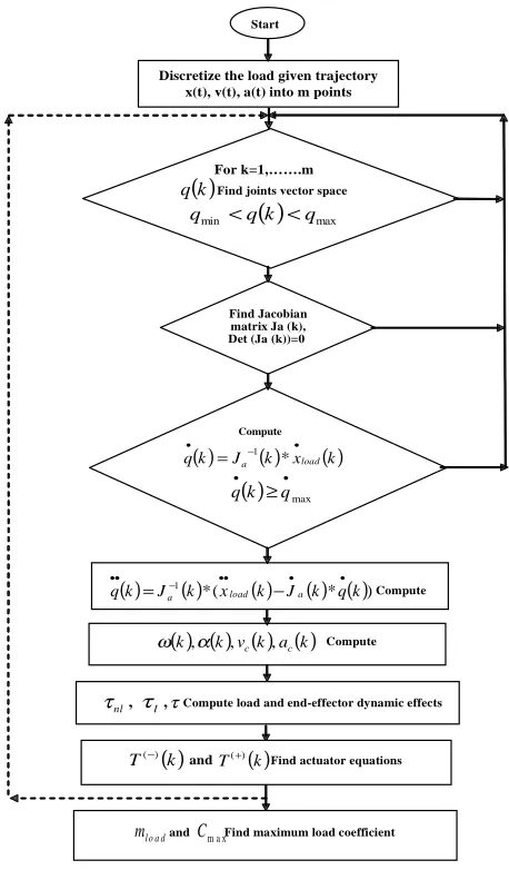
In this Section the computational procedure

for determining the maximum allowable load

is outlined and also flowcharted in Figure 1.

Continuous trajectory of the end effector is

discretized into equally spaced

m

points along

the trajectory, and then the total torque

on

jth

joint at each grid point

τ

j

(

k

)

is obtained

where

k

=

1

,

2

,...,

m

. The joints actuator torque

constraints are formulated based on the typical

joint-speed characteristics of DC motors as

follows:

• − • +

−

−

=

−

=

q

k

k

T

q

k

k

T

2 1 ) ( 2 1 ) (

(16)

where

k

₁

=

T

_s

and

k

₂

=

T

_s

/

ω

_nl

,

T

_s

is the stall

torque and

ω

nl

is the maximum no-load speed

of the motor. If

τ

_nl

(

k

)

satisfies the following

inequality:

) ( ) ( ) ( ( ) ) ( k T k k

T_j + ≤

τ

_nl ≤ _j −

(17)

and if

) ( ) ( ) ( ) ( ( ) ) ( k k T k k

Tj −τnl < j −τnl

−

+

(18)

then the load coefficient at

jth

joint

C

_j

can be

calculated as bellow:

)

(

/

)

(

)

(

)

(

k

T

( )

k

k

k

C

_j

=

_j +

−

τ

_nl

τ

_l

(19)

else, if Equation 18, is not satisfied then:

) ( / ) ( ) ( )

(k T( ) k k k

C_j = − −

τ

_nl

τ

_l

(20)

otherwise, if

nl(k) T( )(k)

+

>

τ

and

0

)

(

k

<

l

τ

then:

)

(

/

)

(

)

(

)

(

k

k

T

( )

k

k

C

_j

=

τ

_nl

−

+

τ

_l

(21)

Start

Discretize the load given trajectory x(t), v(t), a(t) into m points

For k=1,…….m

Find joints vector space

( )k q

( ) max min qk q

q < <

Find Jacobian matrix Ja (k), Det (Ja (k))=0

Compute ( )k J ( )k x ( )k

q a load

• − •

= 1 *

( ) max

• • ≥q k q Compute

( ) 1( )*( ( ) ( ) ( )* )

k q k J k x k J k

q a load a

• • • • − • • − = Compute

( ) ( ) ( ) ( )k,αk,vck,ack

ω

Compute load and end-effector dynamic effects

τ , l τ , nl τ

Find actuator equations

( )k T(+)

and

( )k T(−)

Find maximum load coefficient m a x

C

and

l o a d

m

Under the different conditions, unrealizable

case encountered (e.g., if the desired speed is

too high or the desired trajectory is physically

impossible) and we have:

0

)

(

k

=

C

_j

(22)

The maximum load coefficient at the

jth

joint along the given trajectory is computed as:

}

{

C k k m

Cj,max =min j( ), =1,2,...,

(23)

Finally, the maximum load coefficient for

the mobile manipulator

C

_max

along the given

trajectory is computed from

{

C

j

to

n

}

C

_max

=

min

_j,max

,

=

1

. (24)

where

n

is the number of manipulator’s joint.

The maximum allowable load carrying

capacity for the mobile manipulator is

computed from the following equation:

l load

C

m

m

=

_max

×

(25)

5. SIMULATION STUDIES

To investigate the proposed algorithm, some

simulation studies are presented. In these

studies, a specified trajectory for the load is

assumed. A two-link planar manipulator

mounted on a differentially driven mobile base

is considered as a case study (Figure 2). The

joint actuators are similar and their constants

are

ω

nl =3.5rad /s

and

k

1

=

63

.

22

N

.

m

. For

simulation study two cases are considered in a

situation where the same trajectory for the load

is selected, but a different additional constraint

functions are applied to resolve the motion

redundancy in each case.

5.1. Simulation Model-1

The planar two-link arm is mounted on mobile base at point

F

on the main axis of the base (Figure 2). The position of point

F

relative to world coordinate frame is denoted by

x

f

,

y

f . In this case, the user specified additional constraints

X

_z

=

g q

( )

, are considered as the base position coordinates

F

(

x

_f

,

y

_f

)

.

We combine the additional constraint Equations (A-3), the end effector velocity components Equations (A-4) and the nonholonomic constraint Equation (A-5) (please see Appendix A for details).

Then we rewrite these equations in the matrix

form as mentioned in the Equation (5):

      

 

      

 

=

      

 

      

 

     

 

     



 −

• •

• •

• • • • •

f f e e f f

y x y x y

x J J J

J J J

l Cos

Sin 0

0 0 0 1

0

0 0 0 0

1

1 0

0 1

0 0 )

( )

(

2 1 0 35 34 33

25 24 23 0 0 0

θ θ θ θ

θ

(26) where, the expression of J₂₃,J₂₄,J25,J33,J34 and

35

J are given by:

) sin(

)

sin( _{0 1 2 0 1 2}

1 24

23 =J =−l θ +θ −l θ +θ +θ

J ,

) sin( _{0 1 2} 2

25 = −l θ +θ +θ

J ,

) cos(

)

cos( _{0 1 2 0 1 2}

1 34

33 = J =l θ +θ +l θ +θ +θ J

and J₃₅ =l₂cos(θ₀ +θ₁+θ₂)

By direct calculation, the determinant of the

augmented Jacobian matrix on the left hand side of the Equation (26) is found

) sin( )

(J l0 l1 l2 θ2

Det a = × ×

Hence

J

_ais non-singular provided that

o o ₁₈₀

0

2 ≠ or

θ . That is the two arms are not along the same axis. Suppose that the base length is

l

₀

=

40

cm

, the links length are

cm

l

l

1

=

2

=

50

. Let the initial configuration of

the mobile base is given by:

}

0

,

0

,

0

{

}

,

,

{

x

y

0

cm

cm

rad

q

i

=

f f

θ

=

The initial task vector is considered as

cm

y

x

y

x

X

i

=

{

t

,

t

,

f

,

f

}

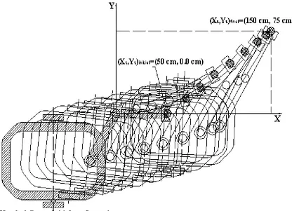
i

=

{

50

,

0

,

0

,

0

}

and desired final task vector at time t=2Secis specified

as

X

_f

=

{

x

_t

,

y

_t

,

x

_f

,

y

_f

}

_f

=

{

150

,

75

,

50

,

75

}

cm

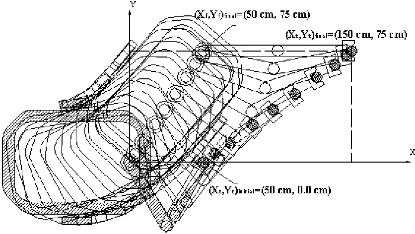
. Notice that final tool tip position is not feasible

without the base motion. The desired task space path is specified as straight lines from initial to final configuration. By simulation study the overall movement of the mobile manipulator is found and shown in Figure 3.

Using the recursive Newton–Euler’s dynamic formulation the torques at the joints of the manipulator are obtained as follows:

2 1 16 1 15 2 2 14 2 13

12 11

1

ω

ω

ω

ω

τ

H

H

H

H

Y

H

X

H

_{f f}

+

+

+

+

+

=

• •

• • •

•

(27)

2 1 25 1 24 2 23 22

21

2 ω ω ω

τ =H Xf+H Yf +H +H +H

• •

• • •

•

(28) where,

[

]

[

(( ) )sin( )

]

) sin(

) (

1 0 1 1 1 2

2 1 0 2 2 2 11

θ θ

θ θ θ

+ +

+

+ + + +

− =

c l

l c

l m l m m

l m l m H

) cos( ) )

((

) cos(

) (

1 0 1 1 1 2

2 1 0 2 2 2 12

θ θ

θ θ θ

+ +

+

+ + + +

=

c l

l c

l m l m m

l m l m H

) cos( )

( _{2 2 2 2}

1 2 2 2

2 2 2

13 I m l ml l m l ml θ

H =c + _c + _l − _c + _l

) sin( )

( _{2 2 2 2}

1

14 l m l ml θ

H =− _c + _l

) cos( ) (

)

( _{2 1}2 _{2 2 2 2}

2 1 1 1

15 I ml m m l m l ml θ

H =c + _c + + _l + _c + _l

) sin( )

( _{2 2 2 2}

1

16 l m l ml θ

H =− _c + _l

) sin(

)

( _{2 2 2 0 1 2}

21=− ml +ml θ +θ +θ

H _{c l}

) cos(

)

( 2 2 2 0 1 2

22 = m l +ml θ +θ +θ

H c l

2 2 2

2 2 2

23 I m l ml

H =c + _c + _l

)

cos(

)

(

_{2 2 2 1 2}

24

m

l

m

l

l

θ

H

=

_c

+

_l

)

sin(

)

(

_{2 2 2 1 2}

25

m

l

m

l

l

θ

H

=

−

_c

+

_l

In the above formulations ₁ 0 1

• •

+

=

θ

θ

ω

and

2 1 0 2

• • •

+

+

=

θ

θ

θ

ω

are the angular velocities of the manipulator links relative to inertial coordinate frame and

l

ci is length of the

ith

link center of mass from its distal joint. The task space trajectory is discretized into equally spaced

m

=

40

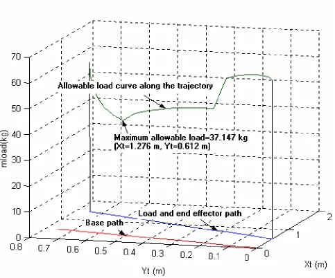
points. Then by the procedure outlined in the Sec. 4 the maximum allowable load of the mobile manipulator is determined (Figure 4). The allowable load carrying capacity for the mobile manipulator at each point of trajectory is determined and maximum allowable load was

found

m

_load

=

37

.

147

kg

at the point

m

x

_t

=

1

.

276

and

y

_t

=

0

.

612

m

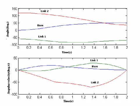
. Also, the corresponding base and links angles and angular velocity variations along the trajectory are illustrated in Figure 5.

5.2. Simulation Model-2

The planar mobile manipulator similar to the Case 1 is considered. The manipulator elbow angle

β

between two arms and end effector orientation relative to the world coordinate frame

α

are used as additional constraint equations. Thus

2 1 0 2 2 1

θ

θ

θ

α

θ

π

β

+

+

=

=

−

=

=

z z

X

X

(29)

The corresponding differential kinematic equation and augmented Jacobian matrix is derived by combining the Equations (A-4), (A-5) and time derivatives of the Equation 29

































=





































































−

−

• • • • • • • • •

β

α

θ

θ

θ

θ

θ

e e f f

y

x

y

x

J

J

J

J

J

J

l

Cos

Sin

0

1

0

0

0

0

1

1

1

0

0

1

0

0

1

0

0

)

(

)

(

2 1 0 35 34 33 25 24 23 0 0 0

(30)

The determinant of the augmented Jacobian matrix on the left hand side of the Equation (30) is found to be

Det

(

J

)

=

l

₀

≠

0

. Therefore, the matrixJis non-singular regardless of the configuration of the mobile manipulator.

The initial task vector is considered

as

X

i

=

{

x

t

,

y

t

,

α

,

β

}

i

=

{

50

cm

,

0

cm

,

0

o

,

120

o

}

and

desired final task vector at time t =2Secis

specified as

}

180

,

60

,

75

,

150

{

}

,

,

,

{

x

y

cm

cm

o o

X

f

=

t t

α

β

f

=

Similar to the Case 1 the final tool tip position is not attainable without the base motion. By considering straight lines from initial to final configuration for the task space variables, the overall movement of the mobile manipulator is determined and illustrated by the simulation study (Figure 6).

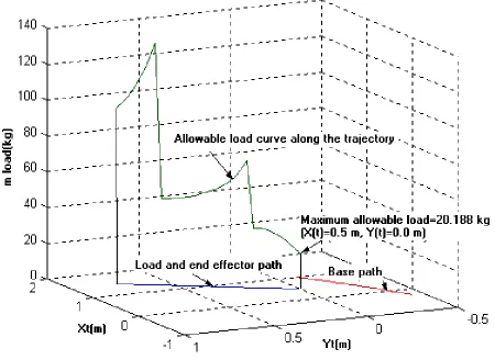
The task space trajectory is discretized into equally spaced m=40points. The allowable load carrying capacity for the mobile manipulator at every point of the trajectory is determined and maximum allowable load is found

kg

m_load =20.188 at point

)

0

.

0

,

5

.

0

(

x

_t

=

m

y

_t

=

m

as shown in Figure 7. The corresponding base and links angle and angular velocity variations along the trajectory are illustrated in Figure 8.

In the above two case studies, the same trajectory for the load is considered. However, in each case different additional kinematical constraint is considered for redundancy resolution. It is seen that load capacity of the mobile manipulator varies along its path depends on the predefined trajectory of the load. Also it can be seen, the maximum allowable load has a different value in each case. Therefore, the value of maximum allowable load for a given trajectory depends on the additional constraint functions that we apply to redundancy resolution. The type of these constraint functions directly depends on the user requirements and can be chosen arbitrarily by considering workspace limitations, obstacle avoidance or optimization criteria.

many functions and libraries for the kinematic and dynamic analysis of robotic manipulators [11,12].

6. CONLUSIONS

The motion planning and dynamic modeling of

mobile manipulators using the augmented Jacobian technique and recursive Newton-Euler method are presented. The application of the algorithm is outlined by simulation studies in detail. In the two case studies a two-link planar differentially driven mobile manipulator with a similar trajectory for the load, and different additional constraint functions for redundancy resolution is considered. In the first

case the base coordinates

x

f and

y

f are applied

as additional constraints and corresponding maximum allowable load is computed

147

.

37

=

load

m

kg. In the second case, the angle between the two links of manipulator and angle of the end effector are considered as additional constraints and corresponding maximum allowable load is computed as mload =20.188 kg. Hence, the results of the case studies are shown that the allowable load is variable along the given trajectory. Also in mobile manipulators in contrast with the fixed base manipulators, the maximum allowable load on a given trajectory has not a unique value. But, a special and unique value may be computed depends on the type of the applied additional constraint functions to resolve the redundancy resolution.

APPENDIX A.

A.1. Case 1 Kinematics

The coordinate of the end effector with respect to joint variables

θ

0

,

θ

1and

θ

2is

)

(

sin

)

(

sin

)

(

cos

)

(

cos

x

2 1 0 2 1 0 1 2 1 0 2 1 0 1 e

θ

θ

θ

θ

θ

θ

θ

θ

θ

θ

+

+

+

+

+

=

+

+

+

+

+

=

l

l

y

y

l

l

x

f e f (A-1)

As explained in Section 5.1 the user specified additional constraints are considered as the base position coordinates f z f z

y

X

x

X

=

=

2 1 (A-2)

by differentiating of Equations (A-2) with respect to time we have:

f z f z

y

X

x

X

• • • •

=

=

2 1 (A-3)

We assume that the speed at which the system moves is low and therefore the two driven wheels

do not sleep sideways. The nonholonomic constraint equation for the manipulator attachment point

F

:

0

)

(

cos

)

(

sin

₀

−

₀

+

0 ₀

=

• •

•

l

y

x

f

θ

_f

θ

θ

(A-4)

where

l

₀is the distance between platform center of mass G and pointF(Figure 2). By differentiating Equation (A-1), the end effector velocity components are as below

)

cos(

)

(

)

cos(

)

(

)

sin(

)

(

)

sin(

)

(

x

2 1 0 2 1 0 2 1 0 1 0 1 2 1 0 2 1 0 2 1 0 1 0 1 e

θ

θ

θ

θ

θ

θ

θ

θ

θ

θ

θ

θ

θ

θ

θ

θ

θ

θ

θ

θ

+

+

+

+

+

+

+

+

=

+

+

+

+

−

+

+

−

=

• • • • • • • • • • • • • •

l

l

y

y

l

l

x

f e f (A-5)

In the inverse kinematics problem, we find

θ

₁and

θ

₂which correspond to a given load position(xe,ye) and a given platform position

(

x

f

,

y

f

)

.

The angle

θ

₂is found by the following expression     − + − − − = 2 1 2 2 2 1 2 2 2 2 ) ) ( ) ((

cos x x y y l l _ll

Arc e f e f

θ

(A-6) By discretizing the robot trajectory into

m

points and by numerical integration of Equation (A-4) The angle

θ

₀can be found. The variables

f

x

•

and

y

_f •

are known, therefore

0

/

))

(

(

sin

)

(

)

)

(

cos(

)

(

(

)

(

)

1

(

0 0 0 0 0

=

×

−

+

=

+

• •

l

dt

i

i

x

i

i

y

i

i

f f

θ

θ

θ

where

i

=

1

to

m

and

dt

=

T

_total

/

m

. Similarly, the angle

θ

₁is given by

(

)

0

2 2

2 2 2

2 1 1

) (

) (

) )(

sin( ) ))( cos( (

cos

θ

θ θ

θ

−

    

  

− + −

− −

− +

=

f e f e

f e f

e

y y x x

y y l

x x l

l Arc

(A-8)

A.2. Case 2 Kinematics

As explained in

Section 5.2 the user specified additional constraints are:

2 1 0 2

2

1z =β =π −θ and X z =α =θ +θ +θ

X

(A-9) In this case, the inverse kinematic of the system is

derived as bellow

β

π

θ

2

=

−

(A-10)

Similar to the Case 1 the base angle relative to the world coordinate frame

θ

₀numerically can be computed by using the Equation (A-7). The angle of the manipulator first link relative to the base main axis

θ

₁ by using the second part of the Equation (A-9) can be calculated as bellow

)

(

_{0 2}

1

α

θ

θ

θ

=

−

+

(A-11)

The base position relative to world coordinate frame at point

F

is calculated by rearranging Equation (A-1). Therefore we have

) ( sin )

( sin

) ( cos )

( cos x

2 1 0 1

2 1 0 1 e

α

θ

θ

α

θ

θ

l l

y y

l l

x

e f f

− + −

=

− + −

=

(A-12) 7. REFERENCES

1. Wang, L. T. and Ravani, B., “Dynamic Load Carrying Capacity of Mechanical Manipulators-Part 1: Problem Formulation”, J. of Dyn. Sys. Meas. and Control, Vol. 110, (1988), 46-52.

2. Yao, Y. L., Korayem, M. H. and Basu, A., “Maximum Allowable Load of Flexible Manipulators for a Given Dynamic Trajectory”, Robotics and Computer- Integrated Manufacturing, Vol. 10, No. 4, (1993), 301-309.

3. Korayem, M. H. and Basu, A., “Formulation and Numerical Solution of Elastic Robot Dynamic Motion with Maximum Load Carrying Capacity”, Robotica, Vol. 12, (1994), 253-261.

4. Korayem, M. H. and Basu, A. “Dynamic Load Carrying Capacity for Robotic Manipulators with Joint Elasticity Imposing Accuracy Constraints”, Robotic and Autonomous Systems, Vol. 13, (1994), 219-229. 5. Carriker et al., W. F., “The Use of Simulated Annealing

to Solve the Mobile Manipulator Path Planning Problem”,

Proc. of IEEE Int. Conf. on Rob. and Autom, (1992), 204-209.

6. Papadopoulos, E. G. and Gonthier, Y., “A Frame Force for Large Force Task Planning of Mobile and Redundant Manipulators”, J. of Robotic Systems, Vol. 16, No.3, (1999), 151-162.

7. Papadopoulos, E. G. and Ray, D. R., “A New Measure of Tip Over Stability Margin for Mobile Manipulators”,

Proc. of IEEE Int. Conf. on Rob. and Autom., (1996), 3111-3116.

8. Ghasempoor, A. and Sepehri, N., “A Measure of Stability for Mobile Based Manipulators”, Proc. of IEEE Int. Conf. on Rob. and Autom, (1995), 2249-2254.

9. Ray, D. A. and Papadopoulos, E. G., “Online Automatic Tip-Over Preventation for Mobile and Redundant Manipulators”, J. of Robotic Systems, Vol. 16, No. 3, (1999), 151-162.

10. Ghariblu, H. and Korayem, M. H., “Mathematical Analysis of Kinematic Redundancy and Constraints on Robotic Mobile Manipulators”, Second International Conference of Applied Mathematics, Tehran, (2000), 502-511.

11. C o r ke, P . I . , “R o b o t i c To o l b o x fo r M ATLAB ”,

Manufacturing Science and Technology,Pinjarra Hills, Australia, (2001).