Research Journal
Volume 11, Iss. 1, March 2017, pages 48–57
DOI: 10.12913/22998624/68460 Research Article
FRICTION MODELING OF AL-MG ALLOY SHEETS BASED ON MULTIPLE
REGRESSION ANALYSIS AND NEURAL NETWORKS
Hirpa Gelgele Lemu1, Tomasz Trzepieciński2, Andrzej Kubit3, Romuald Fejkiel4
1 Faculty of Science and Technology, University of Stavanger, N-4036 Stavanger, Norway, e-mail: hirpa.g.lemu@ uis.no
2 Department of Materials Forming and Processing, Rzeszow University of Technology, Al. Powstańców Warszawy 8, 35-959 Rzeszów, Poland, e-mail: [email protected]
3 Department of Manufacturing and Production Engineering, Rzeszow University of Technology, Al. Powstańców Warszawy 8, 35-959 Rzeszów, Poland, e-mail: [email protected]
4 Stanisław Pigon State School of Higher Vocational Education in Krosno, ul. Rynek 1, 38-400 Krosno, Poland, e-mail: [email protected]
ABSTRACT
This article reports a proposed approach to a frictional resistance description in sheet metal forming processes that enables the determination of the friction coef-ficient value under a wide range of friction conditions, without performing time-consuming experiments. The motivation for this proposal is the fact that there exists a considerable amount of factors that affect the friction coefficient value and as a re -sult building analytical friction model for specified process conditions is practically impossible. In this proposed approach, a mathematical model of friction behav -iour is created using multiple regression analysis and artificial neural networks. The regression analysis was performed using a subroutine in MATLAB programming code and STATISTICA Neural Networks was utilized to build an artificial neural networks model. The effect of different training strategies on the quality of neural networks was studied. As input variables for regression model and training of radial basis function networks, generalized regression neural networks and multilayer net -works, the results of strip drawing friction test were utilized. Four kinds of Al-Mg alloy sheets were used as a test material.
Keywords: coefficient of friction, friction, GRNN, neural networks, RBF network, sheet metal forming.
INTRODUCTION
Regression modelling is one of the most of
-ten used methods to solve problems in engineer
-ing, economics and management science [10, 17, 18]. For instance, mathematical models are utilized to characterize the relationship and to
predict possible fault patterns based on the pro
-cess conditions in the spot welding pro-cess [14]
and to find an input-output relationship in a tung
-sten inert gas welding process [7]. On the other
hand, the wide field of application of the regres
-sion analysis proves there exists no unequivocal definition of regression term [10]. According to Cohen et al. [4] multiple regression analysis is highly general and, therefore, it is a very flexible data-analytic system that may be used whenever
a dependent variable is to be studied as a func
-tion of, or in rela-tionship to, any factors of inter
-est expressed as independent variables. In other words, an advantage of regression in scientific research concerns the possibility of predicting the value of a dependent random variable based on the values of other independent variables and
establishing a functional relation of the
statisti-cal nature. The mathematistatisti-cal complexity of the model and the degree to which it is a realistic model depends on how much is known about the process being studied and on the purpose of the modelling task. A causal analysis allows us to separate the effect of independent variables on
the dependent variables so the unique contribu
-tion of each variable can be examined. Alterna
-tive approaches to stochastic analysis are arti
-ficial neural networks (ANNs) which allows us
to overcome the difficulty arising in the assess
-ment of the complex relationships that is estab
-lished based on empirical analytical models and is based on the empirical non-analytical models. Many ANN architectures have been developed to realize the regression and classification tasks.
The most widespread ones are Kohonen’s net
-works, Multilayer Perceptron (MLP), Radial Ba
-sis Function (RBF) and Generalized Regression Neural Networks (GRNN).
Application of ANNs is widely reported in the literature. Aleksendrić et al. [1] used ANN to
predict the recovery performance of brake fric
-tion materials. The predic-tion of tribological properties of plasma nitride 316L stainless steel using ANN has been studied by Yetim et al. [25]. Gyurova and Friedrich [8] have also predicted
sliding friction and wear properties of polyphen
-ylene sulphide composites. ANN are also used to model and optimize the surface roughness in single point incremental forming [12]. Among
the widespread usage of regression analysis in tri
-bology, it is necessary to put special emphasis on the possibility of the determination of the friction co-efficiency [20] and the determination of the wear rate for different combinations of load, grit size, and sliding distance [5, 13, 24]. To develop a
contact area ratio expression regarding the nomi
-nal pressure, the friction coefficient and relative
sliding of the MATLAB programme was utilized [15]. Regression equations have led to modelling
and predicting the film thickness in contact con
-ditions under the elastohydrodynamic lubrication
[11, 16]. A multiple regression model was applied to analyse the influence of different parameters on the springback phenomenon in the sheet metal forming process [6].
Many authors with a huge success applied
ANNs to nonlinear regression analysis. For in
-stance, application of ANN allowed them to find the relationships between the value of the surface roughness parameters and real contact area under
the different friction conditions [19]. Many re
-searchers applied the ANN models to predict flow
curves in a single step deformation on several ma
-terials [3]. An ANN may solve problems by learn
-ing rather than by a specific programm-ing based on well-defined rules [9].
Friction behaviour in sheet metal forming processing depends on several parameters such as contact pressure, sliding velocity, sheet metal
and tool surface roughness, tool material and lu
-bricant condition. Furthermore, recent studies of authors [13, 14] show that the topography of a surface influences the frictional behaviour of a contact surface and hence its wear. Hence, there is a need to understand better the role of friction and to find factors that essentially influence the friction coefficient values. In this article, the clas
-sical regression and different architectures of neu
-ral networks are implemented to modelling the friction of Al-Mg alloy sheets. To determine the
friction coefficient value, the simple strip-draw
-ing test is realized and the efficiency of different training strategies was studied.
MULTIPLE REGRESSION MODEL
The regression model was built based on the results of strip-drawing tests under lubricated
conditions. The aim of the performed experi
-ments was to find the correlation between the value of surface roughness parameters of the sheet metal and rolls as well as the load pressure on the friction coefficient value. The specimens for the friction tests were made of brass sheet metal and were prepared as strips measuring 20
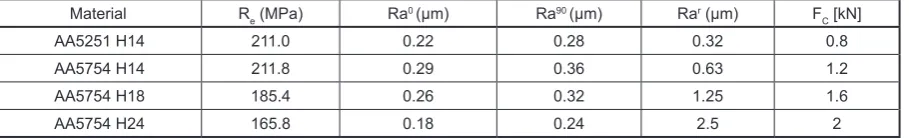
Table 1. Characteristics of tested materials and value of parameters varied during the test
Material Re (MPa) Ra0 (µm) Ra90 (µm) Rar (µm) F
C [kN]
AA5251 H14 211.0 0.22 0.28 0.32 0.8
AA5754 H14 211.8 0.29 0.36 0.63 1.2
AA5754 H18 185.4 0.26 0.32 1.25 1.6
mm in width and about 200 mm in length, cut along the rolling direction of the sheet. The tests were performed using the values of roll surface
roughness (Rar) and clamping force (F
C) given
in Table 1.
The mechanical properties of the sheet
met-al are the main parameters influencing the phe
-nomena that exist between asperities of contact
bodies. The value of yield stress Re (Table 1) is
determined in the uniaxial tensile test. The given
clamping force values are approximated. Appli
-cation of different values of clamping force al
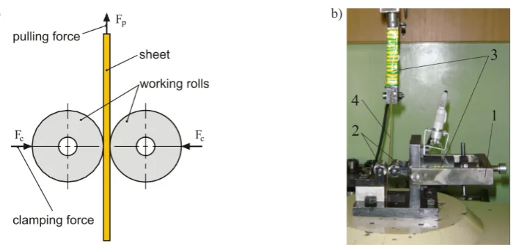
-lows us to build a data set with the wide range of input signals. The sliding veloc ity was set to 2 mm/s. The test conducted in such a way that a strip of the sheet was clamped with specified force between two cylindrical rolls of equal radii (Fig. 1a). The experimental setup is also shown in Figure 1b.
The rolls were made of cold working tool steel. Then when the displacement of moving crosshead of testing machine was engaged, the pulling force and clamping force were recorded continuously using a load cell and a computer
programme. The coefficient of friction µ, defined
as a ratio of the results of the clamping force Fc
and pulling force Fp, was determined using the re
-lationship µ = Fp/2Fc [20]. Surface roughness pa
-rameters were measured by using Taylor Hobson Surtronic 3+ instrument to determine arithmetic
average height along the rolling (Ra0) and
trans-verse directions (Ra90) of the sheet metal. The
arithmetic average height parameter of rolls was measured along the generating line of the roll.
Selecting the factors that have influence on frictional resistance of a sheet metal is necessary
to take into consideration the requirements that
are related with the construction of the regres
-sion model. These requirements boil down to the selection of factors that significantly influ
-ence the frictional resistance and are simultane
-ously independent. Significance of requirement
of particular factors may be verified using elimi
-nation by a posteriori method on the later stage
of model building. As the independent vari
-ables, the clamping force of the rolls and surface roughness parameters of sheet metal and rolls
were taken into consideration. All tested materi
-als were tested for all combinations of variation of surface roughness parameters of the rolls and
clamping forces. A matrix of independent vari
-ables was built on the basis of 80 observations (i.e. n = 80).
The selection of multiple regression model by a posteriori method was carried out by sub
-routine in MATLAB+SIMULINK package.
MAT-LAB is a high-level computer language for sci
-entific application based on matrix formulation. The advantage of an interactive system is that programs can be tested and debugged quickly, allowing the user to concentrate more on the
principles behind the program and less on
pro-gramming itself. Furthermore, MATLAB subrou
-tines can be developed in a much shorter time than equivalent FORTRAN or C programs. The elementary assumptions and methods creation of multiple regression model are introduced below (Equation 1). The linear regression model with
p independent variables X and one dependent
variable Y was established. In further consid
-erations, it is necessary to determine if the re
-ceived model is a good predictor. So the model
a) b)
can be written as [21]:
Y = Xβ + ε
(1)where: Y – vector of observations on the de
-pendent variable Yi (n × 1), X – matrix consisting of a column of ones, which is
labelled 1, followed by the p column vec
-tors of the observations on the independ
-ent variables (n × p), β – vector of param
-eters to be estimated (p × 1), ɛ – random terror vector (n × 1).
The vector of residuals ε reflects the lack of
agreement between the observed Y and the esti
-mated Ŷ:
ɛ
i= Y
i– Ŷ
i (2)The subscript i denotes the observational unit
from which the observations on Y and the p inde
-pendent variables were taken. The conventional
tests of hypotheses and confidence interval esti
-mates of the parameters are based on the assump
-tion that the estimates are normally distributed.
Thus, the assumption of normality of the εi is
critical for these purposes. However, normality is not required for the least squares estimation. The expected value of random error E(ɛ) = 0 and
variance D2(ɛ ) = Iσ2 = 0, where I is a unit ma
-trix, so the elements ɛ must be non-correlated [2]. Because E(ɛ) = 0 the other way of describing the model is as follows:
E(Y) = Xβ
(3)Then, the sum of squares is equal to:
E(Y) = Xβ
(4)The value of estimator β obtained by the least
squares method is equal to b which after substitut
-ing into Equation 2 minimizes to ε’ε.
For the four independent variables, four es
-timators of parameters βi, {i∈N:0<i<5} are
sought, which are determined by the well-known least square estimation. Values of estimators b i, {i∈N:0<i<5} are expressed as:
b = (X
TX
-1X
T)Y
(5)Ifseveral normal equations depend on other
equations then a matrix XTX is singular, so (XTX)
-1 does not exist. Then a smaller number of param
-eters need to be taken into account in the model. The values of estimators can be obtained by least square estimation under the assumption that:
• the form of the model is linear,
• received factors influenced on the friction co
-efficient value are not random and they are in
-dependent from each other,
• the number of received factors to create the
regression model are less than the number of observations,
• the determinant of matrix XTX ≠ 0 otherwise
XTX are non-singular,
• ɛ i is a random variable with the advisable val
-ue equals to 0.
Elements of vector b are the linear func
-tions of observa-tions Yi, i ∈〈1, n〉 and provide
unbiased estimates of the elements of β which
have the minimum variance irrespective of dis
-tribution properties of the errors.
The vector of estimated means of the depen
-dent variable Y for the values of the indepen-dent variables in the data set is computed as:
Ŷ
=Xb
(6)After determination of b and combination with Equation 6, the regression equation gets the form:
(7)
Upon relating the center matrix to the mean values, we find j×y square matrix . Determining the elements of correlation matrix with factors
from the interval (0, 1), the correlation matrix be
-comes:
(8)
(9)
Useful statistics to check is a R2 value of a
regression fit, which measures the proportion of
total variation about the mean Yśr explained by
the regression and it is defined by:
Where both summations are over i = 1, 2,…,
n. Factor R2 is called the square of the multiple
correlation coefficient and shall take the values as high as 1.
The larger the value of R2, the better the fitted
equation can explain the variation in the data. As
-signed regression model has R2 = 0.83371 imply
-ing that 83.371% of the sums of squares can be associated with the variation in these four inde
-pendent variables. According to the literature, the
model with R2 above 80% may be acknowledged
as a good predictor [23]. Analysis of variation (Ta
-ble 2) can be used to check the fitness of friction model and to identify the main effects of design variables.
Therefore, the variation allows determina
-tion of uncertainties related with prognosis of
variable values. Variance as a mean square de
-viation of random variables from their mean value is a measure of a dispersion effect of the probable variable value and it is an irreplaceable testing tool of significance of the whole model.
Under the significance level of α = 0.05 the to
-tal value of F-test (Fischer – Snedecor’s test) of
74.2008 that exceeds the value of F = 2.33, as
read from tables of F-test, confirmed that Equa
-tion 4 is a good predictor. Significance level is
called a probability of a mistake during the esti
-mation of parameter significance that is its prob
-ability to indicate the incorrect estimate of the whole model. Usually the significance level is assumed equal to 0.05.
In the case of lower values, it often occurs that after the estimate of significance level of a parameter, it appears that the significance does not have a sufficiently high level. The higher level of probability may cause that a computed parameter, despite positive significance test, does not fulfil theoretical assumptions of the regres
-sion method. The number of degrees of freedom related with each sum of squares exhibits how much independent information is included in the n independent values Yi, {i∈N:0<i<n} is needed
to specify a sum of squares.
In order to obtain the best prediction quality of
the regression equation, as many variables as pos
-sible should be considered. It can be related the with building of a database of lots of observations and the involved variables in the regression model so that it is possible to analyze the number of variables as low
as possible. The compromise between these contra
-dictory conditions is the selection procedure of the best regression equation. The lowest value of partial F-test (Table 3) is higher than the value read out from the regression table at F = 2.50 under the significance
level α = 0.05. Because the obtained F-test value for
variable X1 is higher than the critical value, it can be accepted that the equation Ŷ =f(X1, X2, X3, X4, X5)
is a final regression model. To ensure better predic
-tion, the model may be improved, for example, by increasing the input variables or introducing mixed
components X1*X2, X1*X3 etc. However, taking into
account high value of square of the multiple correla
-tion coefficient R2 = 83.371% and lower value of the
standard deviation factor of 0.016 the model was ac
-cepted as adequate.
The results of partial F-test value (Table 3) determined after rejection from the regression
model confirmed the significance of all vari
-ables. However, the highest value of partial
F-test is observed after rejection of Ra0 roughness
parameter, so this parameter exhibits the small
-est in formativeness.
Table 2. Results of analysis of variance
Source of variation
Degrees of
free-dom
Sum of
squares squareMean Total F
Generally 79 0.086175
Regression 5 0.071845 0.014369 74.2008
Residue 74 0.01433 0.000194
Table 3. Results of partial F-test analysis
Source of variation Degrees of freedom Sum of squares Mean square Partial F
Regression 5 0.071845
due to Re | Ra0, Ra90, Rar, F
C 1 0.003525 0.003525 18.20079
due to Ra0 | R
e, Ra90, Rar, FC 1 0.025912 0.025912 133.8073
due to Ra90 | R
e, Ra0, Rar, FC 1 0.013834 0.013834 71.43959
due to Rar | R
e, Ra0, Ra90, FC 1 0.00175 0.00175 9.038703
due to FC | Re, Ra0, Ra90, Rar 1 0.016713 0.016713 86.30279
Figure 2 shows comparison of the values of the friction coefficient for AA5754 H18 sheet metal. As shown in the two plots, it compares the values determined by experimental work (Figure 2a) and those predicted by the regression model.
It is possible to observe that the multiple regres
-sion model has greater smoothing properties of
data, while the results of experimental study of the friction coefficient value for particular sets of input variables may possess systematic errors.
NETWORKS MODELS
To build different network models, the Statis
-tica Neural Networks (SNN) were used and di
-verse networks such as MLPs, RBFs and GRNNs
were employed to analyse the data. Next, the net
-work that shows the best performance for the ana
-lysed types of ANNs was selected. The methodol
-ogy of creating MLP for the prediction of value of friction co-efficiency is presented in other works
of the authors [20, 23]. The input variables cor
-responded to the variables used to calculate the classical regression equation (see Section 2). The most important parameter from input variables
is roughness parameter Ra0 (Table 4). The yield
stress value exhibits the smallest effect on the
value of friction co-efficiency. A measure of the
sensitivity of the network is the value of error in
-dicated the quality of the network in the case of absence of a given variable. The more important
input parameter in the learning or validation pro
-cess, the greater the value of the error.
As illustrated in Fig. 3, the RBF networks consisted of three layers. The radial activation functions are implemented in the hidden layer of neurons.
It is most often a Gaussian function:
(11)
where: ||∙|| stands for Euclidean norm and si is a
parameter determining the shape of radial
function.
Radial networks are composed of neurons whose activation functions can be realized using the representation given in the following equation (12):
(12)
The functions φ(||x - c||) are called the radi
-al basis functions. Their v-alues change radi-ally around the center c. RBF networks can model
any non-linear function with using a single hid
-den layer [22].
a) b)
Fig. 2. Value of friction coefficient value for AA5754 H18 sheet metal: a) determined experimentally; b) predicted by regression model
Table 4. The importance of input variables determined for training set
Parameter Variables
Re Ra0 Ra90 Rar F
C
Rank 5 1 2 3 4
Error 0.0155 0.04519 0.0365 0.03361 0.01941
Furthermore, the linear transformation occur
-ring in the output layer can be optimized using
traditional linear modelling techniques. Conse
-quently, during the learning process of RBF net
-work no local minima occur. They are basic prob
-lems during the learning of MLP. RBF networks can be learnt in a very short time compared with that of MLPs.
In the process of training RBF networks, the se
-lection of weights of a hidden layer with an output layer comes down to solving the following equation:
G’w = y
d (13)where: w - sought weights matrix, G’- response
matrix of hidden layer on all training vec
-tors, yd - a matrix of desired responses
for all training vectors.
The solution of Equation 13 can be obtained
by minimizing the square of the norm or absolute value ||yd - wG'||.
GRNNs, which is one of a Bayesian type net
-work [1, 17], is used for a generalized regression purpose. The network consists of 4 functionally different layers: input, radial (for storing centers), regression and output layers. GRNNs use the
method of nuclear approximation in order to real
-ize regression. In GRNNs the Gaussian nuclear functions are arranged in each neurons of hidden layers in such a way that, for each case of training set, there exists one neuron that spans over the case and that is an appropriate Gaussian function.
In the GRRNs the radial neurons represent clus
-ters, not isolated training cases. The algorithm tests each case, assigns it to the nearest radial neuron, and determines the weights for neurons that appear in the third layer. It computes the sum of the values of output variables and the counting of cases assigned to specific cluster.
In order to scale the data to the suitable range
minimax procedure [22], which automatically de
-termine the scale factors, were selected. The num
-ber of training sam ples in the training set (TS)
was 64. The training set consists of values of in
-put variables and corresponds to the value of the friction coefficient. For the purpose of keeping an inde pendent check on the progress of the BP
algorithm, all observations were randomly sepa
-rated from the validation set (VS) which contains
16 training pairs (20% of all training samples).
Fig. 3. The architecture of RBF network
Table 5. Regression statistics for MLP 5:5-11-1:1
Parameter
Learning algorithm Back
Propagation Conjugate Gradients Quasi Newton Levenberg-Marquardt
TS VS TS VS TS VS TS VS
Error Mean -0.0019 0.0011 0.0001 0.0033 0.0033 0.0062 -0.0028 -0.0004
Error S.D. 0.0110 0.0106 0.0198 0.0216 0.0143 0.0139 0.0135 0.0118
ABS Error Mean 0.0086 0.0090 0.0166 0.0185 0.0123 0.0127 0.0107 0.0097
S.D. Ratio 0.3403 0.2919 0.6126 0.5930 0.4411 0.3815 0.4185 0.3241
Correlation 0.9480 0.9623 0.7920 0.8159 0.9077 0.9407 0.9098 0.9506
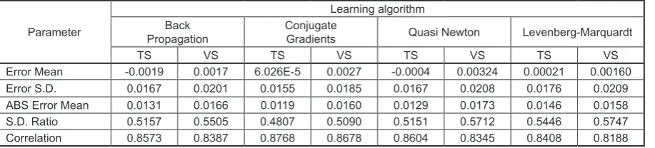
Table 6. Regression statistics for RBF 5:5-14-1:1
Parameter
Learning algorithm Back
Propagation ConjugateGradients Quasi Newton Levenberg-Marquardt
TS VS TS VS TS VS TS VS
Error Mean -0.0019 0.0017 6.026E-5 0.0027 -0.0004 0.00324 0.00021 0.00160
Error S.D. 0.0167 0.0201 0.0155 0.0185 0.0167 0.0208 0.0176 0.0209
ABS Error Mean 0.0131 0.0166 0.0119 0.0160 0.0129 0.0173 0.0146 0.0158
S.D. Ratio 0.5157 0.5505 0.4807 0.5090 0.5151 0.5712 0.5446 0.5747
Different training algorithms were used to train the networks, namely Back Propagation (BP), Conjugate Gradients (CG), Quasi Newton (QN) and Levenberg-Marquardt (LM). In the case of GRNNs, only the training of generalized regression method is available in SNN. The BP algorithm was used with the following settings:
learning rate value was 0.1 and mo mentum val
-ue was set to 0.3 [21]. The quick propagation algorithm was used with the following settings: learning rate value was 0.1 and acceleration value
was set to 2 [22]. As a criterion to stop the train
-ing process, the value of the Root-Mean-Square (RMS) error for validation set was used where the error shows no more decreasing trend. The one
network with the best performance for the anal
-ysed types of ANNs was selected to compare the regression statistics (Tables 5 to Table 7).
Factors necessary to estimate the regres sion model are [22]: data standard deviation ratio (S.D.
Ratio) and the standard Pearson-R coefficient be
-tween the target and actual outputs values. These factors are independently determined for all sets. For a very good model the value of S.D. Ratio amounts to less than 0.1.
It is observed that the used training algorithms has a great impact on the correlation coefficient and S.D. ratio. In the case of MLP network (Table
5), the highest performance is received for the net
-work trained using back propagation algorithm.
The high efficiency of the learning process is con
-firmed by the value of correlation coefficient for verification set that is higher than the training set.
In the case of the RBF network (Table 6), the
Conjugate Gradients was the most efficient train
-ing method. Generally, correlation coefficient and S.D. ratio values for RBF network are very similar for all training algorithms. The values of S.D. ratio (up to 0.48) represent the ability of RBF network to
analyse the regression problems. The best regres
-sion results were found for GRNN network (Table 7). The high value of correlation coefficient (up to
0.96) and the value of S.D. ratio of about 0.25 tes
-tify to the good regression properties of GRNN.
Table 7. Regression statistics for GRNN 5:5-64-1:1
Parameter TS VS
Error Mean -0.00010 0.00043
Error S.D. 0.0083 0.0096
ABS Error Mean 0.0051 0.0069
S.D. Ratio 0.2578 0.2650
Correlation 0.9678 0.9698
Evaluation of neural network model should
take into account both the ability to approxima
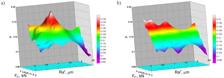
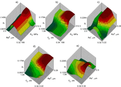
-tion and generaliza-tion. Taking into account only the errors obtained for the training set usually prefers complex models, matching to the training data, but not having the skills to generalize the knowledge. Observation and closer analysis of response surfaces indicate that:
• for the Ra0 parameter in the range of 0.32–1.25
µm, an increase of the parameter value causes
the friction coefficient value to increase (Fig.
4a). After exceeding the value of 1.25 µm, the
friction coefficient starts to decrease,
• a decrease of clamping force value and simul
-taneously the yield stress causes a decrease of the coefficient of friction value (Fig. 4b),
• there is no evident effect of Ra0 parameter val
-ue on the friction coefficient val-ue (Fig. 4c),
• a decrease of clamping force value and simul
-taneously the Ra0 roughness parameter causes
a decrease of the coefficient of friction value (Fig. 4d),
• the maximum value of friction coefficient is
observed for Rar = 1.25 µm, in the case of
higher and lower values of Rar the friction
co-efficients start to decrease (Fig. 4e).
The high value of Pearson’s correlation co
-efficient R and simultaneously low value of S.D.
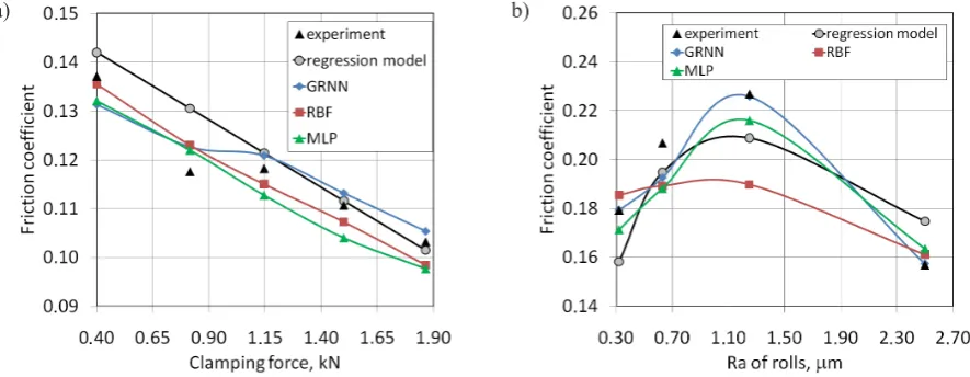
ratio for training set testify good approximation properties of the neural network. Comparison of regression and neural models (Fig. 5a and Fig. 5b) illustrates a better fitting of neural network models to experimental data that are nonlinear.
The best fit of ANN and experimental data is ob
-served for GRNN.
CONCLUSIONS
Although the ANN model better fits the experimental data than the regression model it
does not mean the resignation of an
applica-tion of classical multiple regression. It should be pointed out that the predicted values have to be situated for the range of used values in the building procedure of the regression model. In case of possibly making a choice between the simple and the complex model the simple model
should be preferred unless the other approxi
-mate data is much better. Based on the results of
experiments and neural analyses the main con
-clusions are as follows:
• in the case of MLP network the highest per
-formance is received for the network trained using BP algorithm,
• in the case of the RBF network the Conjugate
Gradients algorithm was the most efficient training method,
• the best performance of the neural model is
observed for GRNN,
• a decrease of clamping force value and simul
-taneously the yield stress causes a decrease of the coefficient of friction value,
• an increase of Ra0 roughness parameter of
sheet metal leads to an increase of the friction
coefficient value.
REFERENCES
1. Aleksendrić D., Barton D.C. and Vasić B. Predic -tion of brake fric-tion materials recovery perfor -mance using artificial neural networks. Tribology International, 43(11), 2010, 2092–2099.
a) b)
Fig. 5. Comparison of friction coefficient value determined experimentally, by regression and ANN model for: a) AA5754 H18 sheet metal (Rar = 0.63 μm); b) AA5754 H14 sheet metal (F
2. Allison P.D. Multiple regression: A primer pine forge press series in research methods and statis-tics. SAGE Publications Ltd., 1999.
3. Bariani P.B., Bruschi S. and Dal Negro T. Predic -tion of nickel-base superalloys’ rheological behav -iour under hot forging conditions using artificial neural networks. Journal of Materials Processing Technology, 152(3), 2004, 395–400.
4. Cohen J., Cohen P., West S.G. and Aiken L.S. Ap -plied multiple regression/correlation analysis for the behavioral sciences. Lawrence ERLBAUM Associates, 2003.
5. Dasgupta R., Thakur R. and Govindrajan B. Re -gression analysis of factors affecting high stress abrasive wear behaviour. Journal of Failure Analy -sis and Prevention, 2(2), 2002, 65–68.
6. de Souza T. and Rolfe B. Multivariate modelling of variability in sheet metal forming. Journal of Mate -rials Processing Technology, 203(1-3), 2008, 1–12. 7. Dutta P. and Pratihar D.K. Modeling of TIG welding
process using conventional regression analysis and neural network-based approaches. Journal of Mate -rials Processing Technology, 184(1-3), 2007, 56–68. 8. Gyurova L.A. and Friedrich K. Artificial neural
networks for predicting sliding friction and wear properties of polyphenylene sulfide composites. Tribology International, 44(5), 2011, 603–609. 9. Kasperkiewicz J. The application of ANNs in cer
-tain-analysis problems. Journal of Materials Pro -cessing Technology, 106(1-3), 2000, 74–79. 10. Kleinbaum D.G., Kupper L.L. and Muller K.E.
Applied regression analysis and other multivari -able methods. PWS Publishing Co., 1988.
11. Kumar P., Jain S.C. and Ray S. Study of surface roughness effects in elastohydrodynamic lubrication of rolling line contacts using a deterministic model. Tribology International, 34(10), 2001, 713–722. 12. Kurra S., Rahman N.H., Regalla S.P. and Gupta
A.K. Modeling and optimization of surface rough -ness in single point incremental forming process. Journal of Materials Research and Technology, 4(3), 2015, 304-313.
13. Lemu H.G. and Trzepieciński T. Numerical and experimental study of frictional behaviour in bend -ing under tension test. Strojniski Vestnik-Journal of Mechanical Engineering, 59(1), 2013, 41–49.
14. Li W. Manufacturing process diagnosis using func -tional regression. Journal of Materials Processing Technology, 186(1-3), 2007, 323–330.
15. Ma B., Tieu A.K., Lu C. and Jiang Z. A finite-element simulation of asperity flattening in metal forming. Journal of Materials Processing Technol -ogy,130–131, 2002, 450–455.
16. Myant C., Spikes H.A. and Stokes J.R. Influence of load and elastic properties on the rolling and slid-ing friction of lubricated compliant contacts. Tri -bology International, 43(1-2), 2010, 55–63. 17. Popko A., Jakubowski M. and Wawer R. Mem
-brain neural network for visual pattern recognition. Advances Science and Technology Research Jour -nal, 7(18), 2013, 54–59.
18. Powroźnik P. Polish emotional speech recognition using artificial neural network. Advances Science and Technology Research Journal, 8(24), 2014, 24–27.
19. Rapetto M.P., Almqvist A., Larsson R. and Lugt P.M. On the influence of surface roughness on real area of contact in normal, dry, friction free, rough contact by using a neural network. Wear, 266(5-6), 2009, 592–59.
20. Stachowicz F. and Trzepieciński T. Zastosowanie sieci neuronowych do wyznaczania współczynnika tarcia podczas kształtowania blach. Informatyka w Technologii Materiałów, 4, 2004, 87–97.
21. Trzepieciński T. Zastosowanie regresji wielokrot -nej i sieci neuronowej do modelowania zjawiska tarcia. Zeszyty Naukowe Wyższej Szkoły Informa -tyki, 9(3), 2010, 31–43.
22. Statistica Neural Networks, Addendum for version 4. StatSoft, 1999.
23. Trzepieciński T. and Lemu H.G. Application of genetic algorithms to optimize neural networks for selected tribological tests. Journal of Mechanics Engineering and Automation, 2, 2012, 69–76. 24. Trzepieciński T. and Lemu H.G. Investigation of
anisotropy problems in sheet metal forming using finite element method. International Journal of Ma -terial Forming, 4(4), 2011, 357–369.