APPROXIMATION OF RANDOM SUMS OF RANDOM VARIABLES IN INSURANCE

(1)

88

Advances in Science and Technology Research Journal

Volume 8, No. 23, Sept. 2014, pages 88–93

DOI: 10.12913/22998624.1120328 Research Article

Received: 2014.07.19 Accepted: 2014.08.18 Published: 2014.09.09

APPROXIMATION OF RANDOM SUMS OF RANDOM VARIABLES

IN INSURANCE

Paweł Wlaź1

1_{Department of Applied Mathematics, Lublin University of Technology, Nadbystrzycka 38, 20-618 Lublin,}

Poland, email: [email protected]

ABSTRACT

The paper deals with approximations of random sums. By random sum we mean a sum of random number of independent and identically distributed random variables. Distribution of this sum is called a compound distribution. The model is especially im-portant in non-life insurance. There are many methods for approximating compound distributions, one of the most popular one is approximation with shifted gamma dis-tribution. In this work we show an alternative way – using kernel density, Fast Fourier Transform and numerical optimization methods – for finding shifted gamma approxi -mations and show results suggesting its superiority over classical method.

Keywords: random sums, Fast Fourier Transform, shifted gamma distribution.

INTRODUCTION

One of main problems in actuary science, which can be very clearly interpreted in the area of insurance, is approximation of random sum of random variables [2, 8]. Formally speaking, let:

Y₁, Y₂, Y₂, ...

be a sequence of identically distributed random variables, with distribution function F_Y and let N be a random variable taking values in the set {0, 1, 2, ...}. Moreover, assume that:

N, Y₁, Y₂, Y₂, ...

are defined on the same probability space and are independent. Then we define sum X as:

Approximation of random sums of random variables in

insurance

Paweł Wlaź

Department of Applied Mathematics, Lublin University of Technology, Nadbystrzycka 38, 20-618 Lublin, Poland, email: [email protected]

ABSTRACT. The paper deals with

approximations of random sums. By random sum we mean sum of random number of independent and identically distributed random variables. Distribution of this sum is called compound distribution. The model is especially important in non-life insurance. There are many methods for approximating compound distributions, one of most popular is approximation with shifted gamma distribution. In this work we show alternative way – using kernel density, Fast Fourier Transform and numerical optimization methods – for finding shifted gamma approximations and show results suggesting its superiority over classical method.

1. Introduction

One of main problems in actuary science, which can be very clearly interpreted in the area of insurance, is approximation of random sum of random variables [2, 8]. Formally speaking, let

be a sequence of identically distributed random variables, with distribution function and let be a random variable taking values in the set

. Moreover, assume that

are defined on the same probability space and are independent. Then we define sum as

(1)

with the convention, that the sum equals whenever .

Now if we think of each as a possible claim in some insurance framework, and if we treat as a number of claims in given time interval, then the distribution of is the distribution of total claims.

Throughout the rest of the paper, we will assume, that is continuous and concentrated on

. In that case, has the same properties. By distribution function of a random variable we mean a function, that for any real is calculated as

It is clear, that , for described by (1), can be expressed in terms of and , namely

(2)

where

(3)

for and is the distribution of random variable taking value with probability .

Formulae (2) and (3) show why it is not in general possible to obtain analytically, even if

(1)

with the convention that the sum equals 0 when-ever N = 0.

Now if we think of each Y_i as a possible claim in some insurance framework, and if we treat N as a number of claims in a given time interval, then the distribution of X is the distribution of total claims.

Throughout the rest of the paper, we will as-sume, that Y is continuous and concentrated on (0, ∞). In that case, X has the same properties.

By distribution function F_Z of a random vari-able Z we mean a function, that for any real x is calculated as:

F_Z(x) = Pr(Z ≤ x)

It is clear, that F_X, for X described by (1), can be expressed in terms of F_Y and F_N, namely

Approximation of random sums of random variables in

insurance

Paweł Wlaź

1. Introduction

(1)

(2)

where

(3)

Formulae (2) and (3) show why it is not in general possible to obtain analytically, even if (2) where:

Approximation of random sums of random variables in

insurance

Paweł Wlaź

1. Introduction

(1)

(2)

where

(3)

Formulae (2) and (3) show why it is not in general possible to obtain analytically, even if

(3) for k > 0 and F*0_{is the distribution of random} variable taking value 0 with probability 1.

Formulae (2) and (3) show why it is not in general possible to obtain F_X analytically, even if one has both F_N and F_Y. The real-life situation is even worse, because one has only samples, not F_Y.

Knowing a good approximation of F_X is crucial for insurer calculating optimal premium [12]. Dis-tribution of X is known as compound distribution.

(2)

89

Advances in Science and Technology Research Journal vol. 8 (23) 2014

PROPERTIES OF COMPOUND

DISTRIBUTION

It is generally accepted to assume F_N is known – or at least known is the class of distributions from which F_N is taken [9].

There are many factors suggesting such an as-sumption; one of them is theoretically and experi-mentally confirmed property of Poisson distribu-tion as a distribudistribu-tion for “rare” cases, what ideally fits the situation in non-life insurance.

So in this paper we will assume, that N has Poisson distribution. Poisson distribution has only one parameter λ, which can be approximated by average number of claims in unit of time, that is why in practice we can think of F_N as known distribution.

Basic parameters of compound distributions, when N is Poisson with parameter λ are easy to obtain, if moments of F₁ are known. Namely [8] one has both and . The real-life situation is

even worse, because one has only samples, not . Knowing a good approximation of is crucial for insurer calculating optimal premium [12]. Distribution of is known as compound distribution.

2. Properties of compound

distribution

It is generally accepted to assume is known – or at least known is the class of distributions from which is taken [9].

There are many factors suggesting such assumption, one of them is theoretically and experimentally confirmed property of Poisson distribution as a distribution for “rare” cases, what

ideally fits the situation in non-life insurance. So in this paper we will assume, that has Poisson distribution. Poisson distribution has only one parameter , which can be approximated by average number of claims in unit of time, that is why in practice we can think of as known

distribution.

Basic parameters of compound distributions, when is Poisson with parameter are easy to obtain, if moments of are known. Namely [8]

(4)

(5)

(6) (7) where is skewness and kurtosis of random variable.

Example 1. Consider having continuous uniform distribution in and let be Poisson with . On fig. 1 we have the density of compound distribution. Details of calculating density functions for compound distributions are

in §4. We can see that in spite of symmetry of all , the distribution of has positive skewness, which is implied by positive skewness of Poisson distribution. In insurance practice usually also are positively skewed, so in general we expect

Figure 1. Density function of compound distribution from example 1

(4) one has both and . The real-life situation is

2. Properties of compound

distribution

distribution.

(4)

(5)

2. Properties of compound

distribution

distribution.

(4)

(5)

2. Properties of compound

distribution

distribution.

(4)

(5)

(7) where: γ₁is skewness and γ₂ kurtosis of random

variable.

Example 1. Consider Y_i having continuous uni-form distribution in (0, 1) and let N be Poisson with λ = 15. On Figure 1 we have the density of compound distribution. Details of calculating density functions for compound distributions are given later. We can see that in spite of symmetry of all Y_i, the distribution of X has positive skew-ness, which is implied by positive skewness of

Poisson distribution. In insurance practice usually also Y_iare positively skewed, so in general we ex-pect strong skewness of the distribution of X. In this example the skewness of compound distribu-tion is about 0.33541, whilst γ₁(Y₁) = 0, γ₁(N) = strong skewness of the distribution of . In this

example the skewness of compound distribution is about , whilst ,

.

3. Approximation with shifted

gamma distribution

Having samples of claims one can easily estimate moments of and . Together with (4)–

(7) basic parameters of are to be estimated with no effort.

Unlike in many other situations, where one-modal continuous distributions are approximated with normal distribution, here normal distribution is not suitable, since normal random variables have skewness equal zero.

To obtain useful distribution with the same three first moments as (and therefore the same expected value, standard deviation and skewness) one has to take simple three parametric one-modal distribution and it is common to consider shifted gamma distribution [8].

A random variable is said to have shifted gamma distribution, if there are real parameters , , , for which – has standard gamma distribution with parameters , . In other words

– has density function

The solution of equations leading to equality of first three moments of distribution of and shifted gamma distributions is as follows

(8)

(9)

(10)

However, there are many situations when this approximation fails. The main problem is, that kurtosis of such approximation always equals

which can be very far from real data, moreover, for too big value of skewness gamma distribution does not fit typical compound distribution. Therefore it is suggested (see [4]) that the approximation with shifted gamma distribution can be applied if

(11)

(12)

The trouble with the above criteria is that it is very hard to estimate , since according to (4)–(7) we have to estimate which – for skewed distributions – cannot be reliably approximated unless sample is extremely big.

Example 2. Consider log-normal with parameters and , that is is normal with mean and standard deviation . Since for -th moment of log-normal distribution we have formula

then we calculate .

Now generate – in statistical R software (see [10]) – 1000 samples from log-normal distribution with

> n = 1000; mu = 0; sigma = 1 > set.seed(1) # to reproduce later > samples = rlnorm(n, meanlog = mu, + sdlog = sigma) > mean( samples^4 )

≈ 0.258199.

APPROXIMATION WITH SHIFTED

GAMMA DISTRIBUTION

Having samples of claims one can easily esti-mate moments of Y₁ and λ. Together with (4)–(7) basic parameters of X are to be estimated with no effort. Unlike in many other situations, where one-modal continuous distributions are approxi-mated with normal distribution, here normal dis-tribution is not suitable, since normal random variables have skewness equal zero.

To obtain a useful distribution with the same three first moments as X (and therefore the same expected value, standard deviation and skew-ness) one has to take simple three parametric one-modal distribution and it is common to consider shifted gamma distribution [8].

A random variable is said to have a shifted gamma distribution, if there are real parameters α, β, x₀, for which (Z– x₀) has standard gamma distribution with parameters α, β. In other words (Z– x₀) has density function:

strong skewness of the distribution of . In this example the skewness of compound distribution is about , whilst ,

.

3. Approximation with shifted

gamma distribution

(8)

(9)

(10)

(11)

(12)

then we calculate .

The solution of equations leading to equal-ity of first three moments of distribution of and shifted gamma distributions is as follows:

.

3. Approximation with shifted

gamma distribution

(8)

(9)

(10)

(11)

(12)

then we calculate .

(8)

.

3. Approximation with shifted

gamma distribution

(8)

(9)

(10)

(11)

(12)

then we calculate .

(9) strong skewness of the distribution of . In this

.

3. Approximation with shifted

gamma distribution

(8)

(9)

(10)

(11)

(12)

then we calculate .

(10)

However, there are many situations when this approximation fails. The main problem is that kurtosis of such an approximation always equals 1.5 ·(γ₁(X))2_{which can be very far from real data,} moreover, for too big value of skewness gamma distribution does not fit typical compound distri-bution. Therefore, it is suggested (see [4]) that the approximation with shifted gamma distribution can be applied if:

Fig. 1. Density function of compound distribution from example 1

(3)

90

strong skewness of the distribution of . In this

.

3. Approximation with shifted

gamma distribution

(8)

(9)

(10)

(11)

(12)

then we calculate .

(11) strong skewness of the distribution of . In this

.

3. Approximation with shifted

gamma distribution

(8)

(9)

(10)

(11)

(12)

then we calculate .

(12)

The trouble with the above criteria is that it is very hard to estimate γ₂(X), since according to (4)–(7) we have to estimate E(Y₁4_{) which – for} skewed distributions – cannot be reliably approx-imated unless sample is extremely big.

Example 2. Consider Y_i log-normal with parameters μ = 0 and σ = 1, that is lnY₁ is normal with mean 0 and standard deviation 1. Since for k-th moment of log-normal distribution we have a formula:

.

3. Approximation with shifted

gamma distribution

(8)

(9)

(10)

(11)

(12)

then we calculate .

then we calculate E(Y₁4_{) ≈ 2980.96.}

Now generate – in statistical R software (see [10]) – 1000 samples from log-normal distribu-tion with:

> n = 1000; mu = 0; sigma = 1 > set.seed(1) # to reproduce later > samples = rlnorm(n, meanlog = mu, + sdlog = sigma)

> mean(samples^4) [1] 4706.422

The obtained estimation of 4-th moment is much bigger than the true value. And for another sample of the same size from the same distribu-tion we have:

> set.seed(2) # to reproduce later > samples = rlnorm(n, meanlog = mu, + sdlog = sigma)

> mean(samples^4) [1] 791.0706

and the obtained value is much smaller than the true 4-th moment. Thus we see that even a reason-ably big sample may fool us about 4-th moment of distribution.

CALCULATING DENSITY OF COMPOUND

DISTRIBUTION WITH FAST FOURIER

TRANSFORM

If the distribution of Y₁ is known, then there exist – using nowadays computer technology – quite an easy way to obtain an approxima-tion of the density funcapproxima-tion of X. Namely, if φ_Z is the characteristic function of Z, that is φ_Z(t) = E(exp(itZ)) (where i is the imaginary unit) and P_N is the probability generating function, that is

P_N(x) = E(xN_{) for}_N_{taking only non-negative} in-teger values, then, in terms of previous sections:

[1] 4706.422

Obtained estimation of 4-th moment is much bigger than true value. And for another sample of the same size from the same distribution we have > set.seed(2) # to reproduce later > samples = rlnorm(n, meanlog = mu, + sdlog = sigma) > mean( samples^4 )

[1] 791.0706

and obtained value is much smaller than true 4-th moment. Thus we see, that even reasonably big sample may fool us about 4-th moment of distribution.

4. Calculating density of

compound distribution with

Fast Fourier Transform

If the distribution of is known, then there exist – using nowadays computer technology

– quite easy way to obtain an approximation of the density function of . Namely, if is the characteristic function of , that is

(where is the imaginary unit) and is the probability generating function, that is for taking only non-negative integer values, then, in terms of previous sections

(13) The equation (13) follows immediately from the fact, that characteristic function of sum of independent variables equals the product of characteristic functions of the variables [1].

If we look at the characteristic function as inverse Fourier transform of density function, and if we look at discrete Fourier transform as an approximation of Fourier transform, then we

obtain the following algorithm (pioneered in [6]), which utilizes computational power of Fast Fourier Transform algorithm [3]:

1. Choose small and large integer ,

calculate vector being

discretization of density function of on interval

2. Calculate .

3. Calculate .

4. Calculate .

Vector is an

approximation of probability function of discretized version of . Terms fft and ifft used here are acronyms for Fast Fourier Transform and Inverse Fast Fourier Transform, respectively.

Due to computational effectiveness of both fft and ifft, integer may be as large as millions, what allows for very small and reduces discretization errors of the procedure. Using some additional R packages (like [5] for discretization) and knowing, that has simple formula

for Poisson with parameter , the whole procedure described above may be scripted as one-liner in R language.

Example 3. In this example we illustrate effectiveness of approximation with shifted gamma distribution. Say, we have

samples from log-normal distribution with parameters and , that is is normal with mean and standard deviation .

Let us generate sample with > n = 200; mu = 0; sigma = 1 > set.seed(1)

> samples = rlnorm(n, meanlog = mu, (13)

The equation (13) follows immediately from the fact that characteristic function of sum of in-dependent variables equals the product of charac-teristic functions of the variables [1].

If we look at the characteristic function as in-verse Fourier transform of density function, and if we look at discrete Fourier transform as an ap-proximation of Fourier transform then we obtain the following algorithm (pioneered in [6]), which utilizes computational power of Fast Fourier Transform algorithm [3]:

1. Choose small h > 0 and large integer M, calcu-late vector y = [y₀, y₁, ..., y_M-1] being discretization of density function of Y₁ on interval (0, M · h). 2. Calculate

[1] 4706.422

Obtained estimation of 4-th moment is much bigger than true value. And for another sample of the same size from the same distribution we have

> set.seed(2) # to reproduce later > samples = rlnorm(n, meanlog = mu, + sdlog = sigma) > mean( samples^4 )

[1] 791.0706

4. Calculating density of

compound distribution with

Fast Fourier Transform

2. Calculate .

3. Calculate .

4. Calculate .

Vector is an

approximation of probability function of discretized version of . Terms fft and ifft

used here are acronyms for Fast Fourier Transform and Inverse Fast Fourier Transform, respectively.

Due to computational effectiveness of both

fft and ifft, integer may be as large as millions, what allows for very small and reduces discretization errors of the procedure. Using some additional R packages (like [5] for discretization) and knowing, that has simple formula

Let us generate sample with

> n = 200; mu = 0; sigma = 1 > set.seed(1)

> samples = rlnorm(n, meanlog = mu,

3. Calculate

[1] 4706.422

Obtained estimation of 4-th moment is much bigger than true value. And for another sample of the same size from the same distribution we have

> set.seed(2) # to reproduce later > samples = rlnorm(n, meanlog = mu, + sdlog = sigma) > mean( samples^4 )

[1] 791.0706

4. Calculating density of

compound distribution with

Fast Fourier Transform

2. Calculate .

3. Calculate .

4. Calculate .

Vector is an

approximation of probability function of discretized version of . Terms fft and ifft

used here are acronyms for Fast Fourier Transform and Inverse Fast Fourier Transform, respectively.

Due to computational effectiveness of both

fft and ifft, integer may be as large as millions, what allows for very small and reduces discretization errors of the procedure. Using some additional R packages (like [5] for discretization) and knowing, that has simple formula

Let us generate sample with

> n = 200; mu = 0; sigma = 1 > set.seed(1)

> samples = rlnorm(n, meanlog = mu,

4. Calculate [1] 4706.422

[1] 791.0706

4. Calculating density of

compound distribution with

Fast Fourier Transform

2. Calculate .

3. Calculate .

4. Calculate .

Vector is an

> samples = rlnorm(n, meanlog = mu, Vector x = [x₀, x₁, ..., x_M-1] is an approximation of probability function of discretized version of X. Terms fft and ifft used here are acronyms for Fast Fourier Transform and Inverse Fast Fourier Transform, respectively.

Due to computational effectiveness of both fft and ifft, integer may be as large as millions, what allows for very small and reduces discretization errors of the procedure. Using some additional R packages (like [5] for discretization) and knowing that P_N has simple formula:

[1] 4706.422

[1] 791.0706

4. Calculating density of

compound distribution with

Fast Fourier Transform

2. Calculate .

3. Calculate .

4. Calculate .

Vector is an

> samples = rlnorm(n, meanlog = mu, for N Poisson with parameter λ, the whole proce-dure described above may be scripted as one-liner in R language.

Example 3. In this example we illustrate effec-tiveness of approximation with shifted gamma distribution. Say, we have n = 200 samples from log-normal distribution with parameters μ = 0 and σ = 1, that is lnY₁ is normal with mean 0 and stan-dard deviation 1.

Let us generate sample with: > n = 200; mu = 0; sigma = 1 > set.seed(1)

> samples = rlnorm(n, meanlog = mu, + sdlog = sigma)

Let us assume for a moment that we have only these data. Let us assume that from some other considerations we fixed the frequency of claims parameter λ equal 15.

(4)

91

Having samples of claims and parameter λ we can of course calculate estimations of E(Y₁k_{), for} k = 1, 2, 3, 4 and – using (4)–(7) – we can find es-timations of EX, y₁(X) and y₂(X). Then, with equa-tions (8)–(10) we find α ≈ 9.3403, β ≈ 0.32337 and x₀≈ –4.6347.

Moreover, left side of (11) is about 0.654 and left side of (12) is about 1.27, so both (11) and (12) are fulfilled.

Now suppose we take p = 0.95 and we want to know what p-quantile of unknown distribution of X is. This is a common task, as it estimates with high probability maximum of total claims in given period. Of course it is to be found as p-quantile of shifted gamma distribution. In this example it equals about 41.345.

How does the latter figure compare to the p-quantile of real distribution of X? If we knew what is the distribution of Y₁, we could calculate the distribution of X – with fft and ifft, and then of course calculate p-quantile which turns out to be about 43.905 so relative error of our estimation is about 5.8.

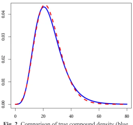
Well, that is only one p-quantile, what about the whole distribution? As usual, an image might be better than numbers. On Figure 2 one can see the density of compound distribution (the blue line, calculated with fft, knowing the distribu-tion of Y₁) and the density estimated with shifted gamma distribution based on samples (the red, dashed line).

Of course one set of samples is not enough, one might suspect some sort of coincidence. We repeat experiment analogous to example 3 – for

seeds equal 1, 2, ... until we find situations which fit (11)–(12) (during the process about 1/5 sets are rejected) – and calculate mean relative error that we have for different tail p-quantiles (and standard deviations of these errors). We use tail p-quantiles, (p close to 1) as these are the most important in the procedure of premium calcula-tions. The results are summarized in Table 1.

Fig. 2. Comparison of true compound density (blue, solid) with its shifted gamma approximation (red,

dashed) based on sample, see example 3

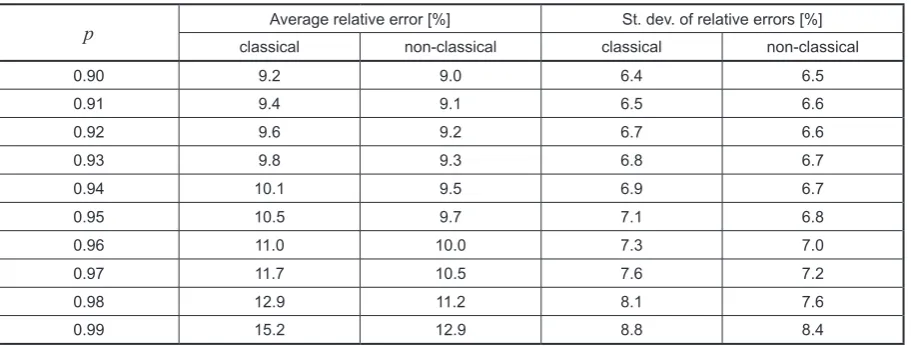
Table 1. Relative errors obtained when p-quantiles of true compound distribution are replaced by their ap-proximations with shifted gamma distribution based on 200-element samples, with (8)–(10). Samples are from log-normal distribution with μ = 0 and σ = 1, for Poisson with λ = 15, averages are calculated after con-sidering 1000 situations which fit (11)–(12)

p Average relative _{error [%]} St. dev. of relative _{errors [%]}

0.90 8.1 5.8

0.91 8.2 5.9

0.92 8.3 5.9

0.93 8.4 6.0

0.94 8.6 6.1

0.95 8.8 6.2

0.96 9.1 6.3

0.97 9.5 6.5

0.98 10.1 6.8

0.99 11.3 7.4

NON-CLASSICAL SHIFTED GAMMA

APPROXIMATION

In this section an alternative method for find-ing approximation of compound distribution with shifted gamma distribution will be described. The motivation for this method may be found in the following example.

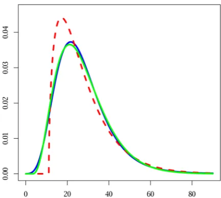
Example 4. Let us assume Y_i are all log-normal with μ = 0 and σ = 1.1. Let N be Poisson with λ = 15. The density of X (calculated with fft) is illus-trated on Figure 3 – solid blue line (partly shad-owed by green line).

After calculating EX, σ(X) and y₁(X) we can find α ≈ 1.59097, β ≈ 0.0971156, and x₀ ≈ 11.0866 for approximation with shifted gamma distribution. The density of shifted gamma dis-tribution for these parameters is pictured with dashed red line on Figure 3. As we see, the lines are far from fitting.

Now look at the green solid line at the same Figure 3. That also is the density of gamma

(5)

92

tribution, this time with parameters α ≈ 3.88213, β ≈ 0.160105, and x₀ ≈ 3.08835. This green line is very close to the line of true density of X.

In the example 4 it was not very hard to ob-tain better than classical shifted gamma approxi-mation, since we know the exact distribution of X (due to fft calculations) and we can minimize maximum of absolute value of differences be-tween distribution functions.

In the real insurance work there is one more problem – we do not have distribution of Y_i, only samples of values of Y_i. The algorithm that we propose in this work is as follows:

1. Find approximation of density of Y_i, basing on samples, let F be distribution function corre-sponding to that density.

2. Basing on density from step 1, find approxi-mation of distribution of X.

3. If by Fα,β,x₀ we denote the distribution func-tion of shifted gamma distribufunc-tion with shape parameter α, rate parameter β and shift param-eter x₀, then find

corresponding to that density.

2. Basing on density from step 1, find approximation of distribution of .

3. If by we denote the distribution function of shifted gamma distribution with shape parameter , rate parameter and shift parameter , then find , and minimizing

(14) And here are some explanations concerning above three steps.

5.1. Density based on samples.

To find an approximation of unknown distribution of claim size based on samples we use Gaussian kernel density estimation which approximates unknown density

with mean of normal densities ,

where parameter is selected according to method of Sheather and Jones [11].

5.2. Compound distribution based on density of claim size.

In this step – as it was mentioned at the beginning of the paper – we assume that frequency of claims is Poisson with given parameter , and having calculated density of claim size we then proceed just in a way described

in §4.

5.3. Optimizing parameters.

To minimize (14) we use general-purpose Nelder-Mead method [7]. This method needs starting point (in this case three-dimensional). Our proposition is to take a few starting points lying between parameters of classical shifted gamma distribution and parameters of gamma distribution with no shift (taking – based only on mean and standard deviation) and choose the one giving best result.

Figure 3. Motivation for non-classical shifted gamma approximation: blue solid line is the density of compound distribution ( log-normal with , , – Poisson with ); red dashed line is the

density of shifted gamma approximation obtained with (8)–(10); green solid line is another shifted gamma, apparently better fitting than the red one

, corresponding to that density.

in §4.

and corresponding to that density.

in §4.

minimizing: corresponding to that density.

in §4.

(14) And here are some explanations concerning the above three steps.

Density based on samples

To find an approximation of unknown distri-bution of claim size Y_i based on samples y₁, y₂,

..., y_n we use Gaussian kernel density estimation which approximates unknown density with mean of normal densities N(μ = y_i, σ = h), where param-eter h is selected according to method of Sheather and Jones [11].

Compound distribution based on density of claim size

In this step – as it was mentioned at the be-ginning of the paper – we assume that frequency of claims is Poisson with given parameter λ, and having calculated density of claim size we then proceed with the algorithm using fft.

Optimizing parameters

To minimize (14) we use general-purpose Nelder-Mead method [7]. This method needs starting point (in this case three-dimensional). Our proposition is to take a few starting points ly-ing between parameters of classical shifted gam-ma distribution and parameters of gamgam-ma distri-bution with no shift (taking x₀= 0 – based only on mean and standard deviation) and choose the one giving best result.

Example 5. In this example we fix μ = 0 and σ = 1, generate n = 200 claims from log-normal dis-tribution. If conditions (11)–(12) are not met, repeat generation. After successful generation, taking λ = 15 as frequency of claims we calculate exact distribution of X, classical shifted gamma distribution based on samples and non-classical gamma distribution based on samples. We then calculate chosen p-quantiles and calculate rela-tive errors. The above procedure is repeated times and average relative errors and their standard de-viations are obtained. The results are summarized in Table 2.

CONCLUSIONS

The presented calculations and illustrations show that it makes sense to use an alternative way to find shifted gamma approximations of com-pound distributions. Of course our novel method is much more cumbersome than the classical method, but calculating premium in real environ-ment does not have to be done in seconds.

The method still needs much more evidence, especially its usefulness for other types of dis-tributions used for modelling claim size should be checked.

Fig. 3. Motivation for non-classical shifted gamma ap-proximation: blue solid line is the density of compound distribution (Y_ilog-normal with μ = 0 and σ = 1.2, N – Poisson with λ = 15); red dashed line is the density of shifted gamma approximation obtained with (8)–(10); green solid line is another shifted gamma, apparently better fitting than the red one