INTRODUCTION
Turning is one of the oldest and most adaptive procedures for production of circular components with just one cutting tool. The products which are usually created by turning process has a wide range from tiny screws for glasses to huge shafts in hydroelectric power plants. The turning is fre-quently conducted by a lathe in which the work piece is attached to the spindle from one side and the tailstock from the other side. The cutting tool is moved through a line, parallel or vertical to the workpiece and is subjected to a linear displace-ment while the workpiece is rotating.
As mentioned, during turning process, the tool and workpiece contacts with each other and a mutual force is created in the contact area.
Some-times, this dynamical force leads to unwanted vibrations called self-excited chatter. The self-ex-cited or regenerative chatter is produced because the machined surface is wavy which generates a vibrating cutting force in the next rotation, in addition this vibrating force itself creates a wavy surface too. This process regenerates itself be-cause the cutting force always vibrates due to the previous wavy surface. The relative movement between the tool and workpiece will continue un-til the chatter is fully developed and the final ma -chined surface will be completely wavy [1].
On the other hand, there is another type of chatter called forced-chatter. It occurs when an external force motivates the structure. The self-generative chatter can usually be prevent-ed through changing the cutting parameters in-Volume 13, Issue 3, September 2019, pages 217–228
https://doi.org/10.12913/22998624/111705
System Identification and Model Predictive Control
of the Chatter Phenomenon in Turning Process
Atiyeh Karimipour
1, Mohsen Emami
11 Behbahan Khatam Alanbia University of Technology, Iran
* Corresponding author’s e-mail: [email protected]
ABSTRACT
Chatter is a series of unwanted and extreme vibrations which frequently happens during different machining pro
-cesses and impose variety of adverse effects on the machine-tool and surface finish. Chatter has two main types
namely forced-chatter and self-existed chatter. The forced-chatter has an external cause; however, self-exited
chat-ter has no exchat-ternal stimuli, rather it is created due to the phase difference between the previous and current waves
on the surface of the workpiece. Due to the self-generative nature of this type of chatter, its recognition and
pre-vention is much more difficult. For preventing self-exited chatter its model should be available first. The chatter
is usually simulated as a one degree of freedom mass-spring-damper model with unknown parameters that they should be determined somehow. In this paper, the parameters of the tool equation of motion i.e. mass, damping,
and stiffness coefficients of the system are predicted through a wavelet-based method online, and then based on the achieved parameters, the system is controlled via Model Predictive Control (MPC) approach. For the validation, the algorithm is applied to 25 different experimental tests in which the acceleration of the tool and cutting force
are measured via an accelerometer and a dynamometer. By investigation of the SLDs generated by the predicted
parameters, the presented system identification method is validated. Also, it is shown that the chatter vibration is completely restrained by means of MPC. For investigation of the MPC performance, MPC algorithm is compared
with PID controller and simulations has indicated a much stronger performance of MPC rather than PID controller
in terms of vibration attenuation and control effort.
Keywords: turning process, chatter phenomenon, system identification, discrete wavelet transform, and model
predictive control
Research Journal
Accepted: 2019.08.20cluding the spindle speed, depth of cut and feed rate. Whereas, the forced-chatter usually can be vanished by removing or adjusting the external force. All types of chatter have many destructive effects such as increasing cutting forces, poor surface finish, decreasing of the tool and lathe lifetime, imprecise dimensions of the product, and load noises [2].
Until now, many researchers have proposed different methods for coping with chatter. The first step for dealing with chatter is to extract a model which can appropriately describe its behavior. But, since it is not possible to predict the exact mechanics and dynamics of cutting, a complex model which can define the complete metal cut -ting dynamics has not been suggested yet [3]. The analysis of chatter includes modeling of the tool and workpiece interaction and modelling of the cutting force which together make a closed-loop dynamical model for turning. After derivation of a model, analytical methods are used to deter-mine the stability status of the process. The curve which determines the stability status of the op-eration is called the Lobe Diagram. This diagram shows stable and unstable zones in the cutting pa-rameters space including spindle speed and depth of cut [4]. For recognition of the stability status of a process by this method, the exact structural pa-rameters of the system have to be specified. One of the most common methods for obtaining the structural parameters is the impulse hammer test. However, according to [5], the structural parame-ters attained by this method are just an estimation of the real coefficients and therefore, always an uncertainty should be considered in the derived model. Otherwise, it is possible that a set of depth of cut and spindle speed located in the stale zone leads to an unusable process because of not con-sidering the uncertainty [6]. Therefore, for a cer-tain turning operation especially when the surface finish has a great importance, an online system identification model along with a reliable control approach is vital for coping with system nonlin-earities and other uncertainties.
There are numerous control approaches for stabilizing chatter, but in these days, the need for better controlling chatter is increasing because there is a pressure on industries for increasing of the productivity, and accuracy, and decreas-ing of the production costs. There are two main ways of controlling of chatter which are passive and active control approaches. In passive meth-ods, some devices are used to absorb the surplus
of the energy including vibration absorbers, fric-tion dampers, mass-dampers or tuned dampers. These devices have frequently lower rigidity and can damp the chatter vibrations. In passive meth-ods, dynamical vibration absorbers or tuned mass dampers are wildly utilized in practical applica-tions in comparison with other methods. Tobias in [7], has presented several practical methods and their effect on the stability of the process in which the vibration absorber is attached to the different parts of the machine-tool. Passive control meth-ods of chatter vibration have many advantages such as low cost, not needing any external energy and easy implementing. But, for more accurate performance the dampers in TMDs need to be tuned online like in active control approaches.
In active control methods, chatter vibrations are actively identified by continuous monitoring of the process, and when it is necessary, the re-quired changes are applied to the system. Some researchers have proposed some techniques that the system parameters such as depth of cut and spindle speed are changed during the process in accordance with the control algorithm needs. For instance, Lin and Hu [8] has presented a method in which the feed rate and spindle speed are al-tered for vanishing chatter. Frumusanu and et al. [9], have offered a control method based on the real-time monitoring of the cutting force.
The main objectives of the present work are the parameter estimation of the system model and chatter vibrations control. For the parameter estimation, first the discrete wavelet transform of the displacement, velocity, acceleration, and force signals are calculated. Then, by putting the achieved coefficients in the system equation of motion and solving it, the mass, damping, and stiffness coefficients of the system are extracted. For controlling of the chatter phenomenon, based on the attained structural parameters, the Model Predictive Control (MPC) algorithm is applied. Finally, the performance of the MPC and PIC controllers are compared.
The main features of the proposed method are:
• For the system identification there is no need for any impulse hammer test or other previous information and the parameters are extracted online during the process based on the cutting force and acceleration signals. So, they can adapt with any new cutting conditions.
In section 2, the dynamics governing the chat-ter phenomenon and the stability lobe diagram (SLD) are presented. In sections 3 and 4, the sys-tem identification approach and the control proce -dure are described. Next, in section 5, the results of applying proposed algorithm on real signals are described, and finally in section 6, the conclu -sion of the present work is expressed.
THE CHATTER THEORY
The regenerative chatter forms due to the in-teraction between the metal cutting process and the machine-tool. This type of chatter occurs near the dominant natural frequency of the ma-chine-tool. The excitation of this mode leads to the relative movement between the tool and the workpiece. This relative movement can be mod-eled as a linear one-DoF system as can be seen in Fig. 1. In this figure, m, c, and k are the mass, damping, and stiffness coefficients of the system. Also, y(t) is the wave formed during the current revolution and y(t-τ) is the wave formed during the previous workpiece revolution. The phase dif-ference between y(t) and y(t-τ) is the main cause of chatter in the turning. If these two waves have the same phase, no vibration will grow in the sys-tem because, the variations in the chip thickness will be very small and negligible. From the en -ergy point of view, when the system is marginally stable, the produced and the dissipated energy becomes equal. Therefore, when no phase dif-ference exists, there is no surplus of energy and so the process will be stable. On the other hand, when the waves do not have the same phase, be-cause the entered energy to the system is more than the dissipated energy, the vibration grows on the workpiece and the system will be unstable.
If it is considered that the tool is flexible and the workpiece is rigid the equation of motion be-comes (Fig. 1):
mÿ(t) + cẏ(t) + ky(t) = Ff (1)
Ff = Kfb[y0 - y(t) + y(t - τ)] (2)
in which y(t) (m) is the displacement of the tool along y direction. b(m) is the depth of cut, τ(s) is the period between two con-secutive revolution, and y(t) - y(t-τ) (m) is the chip thickness which is not constant and is a variable of time. Also, Ff is the
cutting force and Kf is the cutting coeffi -cient along the y direction [4].
By applying Laplace Transform on the left side of equation (1):
(3)
G(s) is achieved which is the open loop trans-fer function of the system. Therefore, The Laplace Transform of the closed-loop system becomes:
(4)
The term e-τs is due to the presence of time de-lay in the main equation (1). For finding the criti -cal depth of cut which puts the system in the criti-cally stable state, the denominator of the closed loop transfer function of Eq. (4) or the character-istic equation of the system is set to zero. Namely:
1 + blimKfG(s)(1- e-τs) = 0 (5)
In which blim is the critical depth of cut. In the critical state, the real part of the roots of Eq. (5) are zero and they have just imaginary part. There-fore, s is set to jw. It means:
1 + blimKfG(jw) ∙ [1 - cos(-wτ) - jsin(-wτ) = 0 (6) The real and imaginary parts of Eq. (6) have to be simultaneously zero. So, by considering G(jw) = Re(G(jw)) + Im(G(jw)) and separating real and imaginary parts, it results:
Real part:
1 + blimKf[Re(G(jw))(1 - cos(wτ)) -
- Im(G(jw))sin(wτ)] = 0 (7) Imaginary part:
blimKf[Re(G(jw))sin(wτ) +
+ Im(G(jw))(1 - cos(wτ))] = 0 (8) Then, after several mathematical manipula-tions the following condimanipula-tions are extracted: Fig. 1. One DoF mass-spring-damper model of the
(9)
(10)
(11)
In Eq. (10), ω and ε are the cutting tool fre-quency and the phase shift between the current and previous waves respectively. Also, k is the se-lected number of lobe that can be varied between 1 and the maximum spindle speed [10].
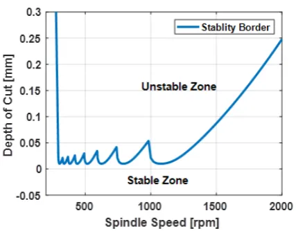
Now, according to Eqs. (9-11), the border be-tween stable and unstable regions of the turning operation can be drawn which is called the Stabil-ity Lobe Diagram or SLD. Figure 2 shows a sam -ple SLD. The SLD separates two regions of stable and unstable cutting operation for different spin -dle speed and depth of cut. If the spin-dle speed and depth of cut are chosen such that they locate under the lobes, the operation is stable, the finish surface is smooth, and low dynamical forces will be applied on the machine-tool. Therefore, by se-lecting a set of suitable spindle speed and depth of cut the chatter vibrations will be prevented.
SYSTEM IDENTIFICATION
Although, stability lobe diagram provides the possibility to predict the stability status of the turning system, this diagram is accurate only
when the exact structural parameters of the sys-tem are available. However, this information is not always known or accurate because of several reasons. First of all, the impact hammer which is needed for determining structural parameters of the system might not be available especially in factory environments. Second of all, by every po-tential change in the process for example, chang-ing of the tool or the workpiece, these parameters will experience alterations and they will not re-main constant for every operation. And finally, even if the system parameters are provided at the beginning of the process, they might change dur-ing turndur-ing because there are many nonlinear fac-tors included in the dynamics of the system which are not considered in the equation of motion [11].
In this paper, a method is presented based on the discrete wavelet transform (DWT) for de-termining the structural parameters based on the cutting force and acceleration of the tool. The main advantage of this method is that it does not need any impact hammer test. In addition, since the parameters are being measured throughout the process, they are changed continuously along with any in-process variation that might happen throughout the process.
If the dynamical equation is considered as (Eq. 1):
mÿ + cẏ + ky = Ff (12)
First DWT coefficients of y, ẏ , ÿ, and F are calculated, then by substituting them in Eq. (12) and solving the resulting algebraic equation, m, c, and k can be achieved.
Therefore, for expanding discrete signals by
DWT in space ,
fol-lowing formula can be utilized [12]:
(13)
In which f[n] is the discrete signal, ϕjn, k[n] is
the scaling function, and ψj,k[n] is the wavelet
func-tion. By taking the scaling and wavelet functions, the wavelet coefficients can be simply achieved by calculating the inner product of the discrete signal and scaling and wavelet functions i.e.:
(14)
(15)
Fig. 2. A sample SLD. Lobes for different spindle
speeds and depths of cut are shown. The line is the stability margin. The upper zones of the line are
Eq. (4) is called approximants coefficients and Eq. (5) is called detail coefficients. The dilation ver -sion of the scaling function is determined as:
(16)
In which hϕ is the impulse response of a low pass filter. After some mathematical manipulations it results that the approximate coefficients can be calculated as follows which is a faster way than Eq. 14: (17)
Similarly, for detail coefficients it results:
(18)
According to Eq. (12), the displacement, velocity, acceleration, and force signals are needed for determination of system parameters. Acceleration and force signals are measured by accelerometer and dynamometer sensors. But, for accessing to displacement and velocity, the acceleration signal should be integrated. It is recommended to use a noise filtering method before integration, because, probably the acceleration signal includes several noise contents and integration will lead to noise intensification. By substitution of detail and approximate coefficients of y, ẏ , ÿ and F in Eq. (12), it results:
(19)
In Eq. (19), Wϕsli and Wψsli are i th approxi-mate and detail coefficients of the signal s (y, ẏ,
ÿ̈, or F) in the selected level of l [13].
Selecting an appropriate level of decomposing is important, because those coefficients should be chosen that can properly describe the dynamics of the system in the chatter mode. Since chatter hap-pens near the natural frequency of the lathe, and the natural freaquncy of the used apparatus is about wn = 400 Hz, level two is selected. Because, the sample rate was 1000 Hz, so the maximum frequency that can happen is 1000 Hz. One level decomposition leads to two subspaces of 0 to 500 Hz and 500 to 1000 Hz. Again, another decomposition of approxi-mate coefficients results in two other subspaces of 0 to 250 and 250 and 500 Hz. This level is selected because wn exactly lies in these frequency band.
Finally, by solving of the system of equations of Eq. (19) via least mean square method, the un-known parameters of m̂, ĉ, and k̂ can be calculated. After determination of structural parameters, the system must be controlled in order to avoid adverse effects of chatter vibration which is de -scribed in the next section.
MODEL PREDICTIVE CONTROL (MPC)
In this work, model predictive control is used for controlling unwanted vibrations of chatter. The main goal of the Model Predictive Control is calculating the future trajectory of variable u for optimization of the future behavior of the system output i.e. y. In this type of controller, the model of the process is used for predicting the output of the system in the future. The control effort is achieved by minimization of a cost function. Some of the merits of this controller are: 1 - using basic con-cepts of control in designing, 2 - simple adjusting of the controller gains, 3 - the ability to expand for complex, non-minimum phase and delayed sys-tems easily, 4 - the ability to expand for MIMO systems, 5 - having a feedforward controller in or-der to compensate for measurable disturbances, 6 - easy control rule implementation, 7 - considering control signal, output, and state constraints in the design, and 8 - very useful in applications that the desired future trajectory is known.1. It can control unstable and non-minimum phase processes such as turning operation. 2. Having a forward-looking approach, this
controller can avoid noises and disturbances. Since, machine-tools are placed usually in in-dustrial environments and the sensors are ex-posed to different sources of noise.
3. After designing, a very simple and easy-imple-menting control rule will be extracted.
4. It can work in real-time applications with no trouble.
In here, SISO systems are considered, be-cause in the turning process there is a linear sec-ond order system with one input and one output.
The state space model of system is:
xm(k + 1) = Amxm(k) + Bmu(k)
y(k) = cmxm(k) (20)
In which u is the input, y is the process output, and xm is the state space vector with n elements. In here, according to the receding horizon con-trol principle in which just previous information is needed for predicting and control, it is assumed that the input u cannot directly affect the output and so Dm = 0.
By considering, Δxm(k)= xm(k)- xm(k - 1)
and Δu(k) = u(k) - u(k - 1), Eq. (20) will be: Δxm(k + 1) = AmΔxm(k) + BmΔu(k) (21)
By definition of a new set of state variables as: x(k) = [Δxm(k)T y(k)T] (22)
The new state space is:
(23)
In which . The triple of
(A, B, C) in Eq. (23) is called augmented model used in model predictive control algorithm.
For computing future output based on the control future signal, ki is considered as the
cur-rent time, and Np as the number of predicted
fu-ture outputs called prediction horizon. This num-ber also shows the length of the optimization win-dow. Nc is the control horizon which shows the
number of parameters used for predicting future control trajectory. The future control inputs are: Δu(ki), Δu(ki + 1), …, Δu(ki + Nc - 1), and
fu-ture state variables are: x(ki + 1 | ki), x(ki + 2 | ki
), …, x(ki + m | ki ), …, x(ki + Np | ki) in which
x(ki + m | ki) is the predicted state variable in the
time ki + m by possessing information of x(ki). Also, NC ≤ Np.
By substitution of the above variables in the state space of Eq. (23), it results:
x(ki + 1 |ki) = Ax(ki) + BΔu(ki)
x(ki + 2 |ki) = Ax(ki + 1 |ki) + BΔu(ki + 1)
= A2x(k
i) + ABΔu(ki) + BΔu(ki + 1)
...
x(ki + Np | ki) = ANp x(ki) + ANp-1BΔu(ki) + ANp-2BΔu(ki + 1) + ... + ANp- Nc BΔu(ki + Nc - 1)
(24)
The predicted output variables can be determined by Eq. (24) as:
y(ki + 1 |ki) = CAx(ki) + CBΔu(ki)
y(ki + 2 |ki) = CA2x(ki) + CABΔu(ki) + CBΔu(ki + 1)
y(ki + 3 |ki) = CA3x(ki) + CA2BΔu(ki) + CABΔu(ki + 1) + CBΔu(ki + 2)
...
y(ki + Np | ki) = CANp x(ki) + CANp-1BΔu(ki) + CANp-2BΔu(ki + 1) + ... + CANp- Nc BΔu(ki + Nc - 1)
(25)
If two vectors are defined as follows:
Y = [y(ki + 1 |ki) y(ki + 2 |ki) y(ki + 3 |ki) ... y(ki + Np | ki)]Npx1T
ΔU = [Δu(ki) Δu(ki + 1) Δu(ki + 2) Δu(ki + Nc - 1)] Ncx1T
(26)
By compacting Eqs. (24) and (25) and considering Eq. (26), it results:
Y = Fx(ki) + ΦΔU (27)
(28)
The aim of horizon control is to close up the control output to the reference signal of r(ki) provided
that the reference signal is constant in the optimization window. From this, an error function will be
defined by the aim of minimizing. If the reference signal is considered as: , the cost function of J that contains the aim of control will be:
J = (Rs - Y)T (Rs - Y) + ΔUT R̅ΔU (29) The first term in Eq. (29) is related to the minimization of the error between the predicted output and the reference signal while the second term reflects the importance of ΔU magnitude in the cost function. R̅ is a diagonal matrix in the form R̅=rw INc×Nc (rw ≥ 0) in which rw should be adjusted such that the
closed-loop system would have a proper performance.
The cost function of J has to be minimized. For looking for the suitable ΔU that can minimize J, by considering Eq. (27), Eq. (29) can be rewritten as:
J = (Rs - Fx(ki))T (Rs - Fx(ki)) - 2ΔUT ΦT (Rs - Fx(ki)) + ΔUT (ΦT Φ + R̅)ΔU (30)
By differentiating Eq. (30) and equating to zero, the optimize answer for ΔU is achieved as: ΔU = (ΦT Φ + R̅)-1ΦT (R
s - Fx(ki)) (31)
Rs is a vector containing reference point information as = R̅sr(ki), [14].
ΔU is the designed and optimized MPC control input which can be applied to the state space of Eq. 20.
RESULTS AND DISCUSSION
For validation of the proposed method, 25 experimental tests have been designed and con-ducted. In these tests, the cutting parameters are set such that the spindle speed is set to 200, 600, 1000, 1400, and 1800 rpm and the depth of cut is set to 0.25, 0.5, 1, 2, and 4 mm. All tests are performed in the wet condition. The lathe used is a CNC of type TME0. The material of workpieces is AISI1045, and each workpiece has a length of 250 mm and a diameter of 45 mm. In each opera-tion, 50 mm of each workpiece is machined. The soluble oil of Mobilcut100 with the concentration of 5% and the flow rate of 2 liter/min is utilized as the lubricant. The cutting tool has a ISO standard of DNMG 15 06 08-PR 4225 and the tool holder model is PDJNR2020K15. For gathering tool ac -celeration, an accelerometer of type AC102-1A which has a sensitivity of 100 mV/g and a data logger of type 4-channel NI-USB 6009 are used. In addition, a voltage amplifier of type IEPE is employed for strengthening the output data of accelerometer. Finally, the cutting forces are col -lected by a dynamometer of type 9257A which
is a three-axis piezoelectric Kistler dynamometer. The data gathering is performed by the sample rate of 1000 Hz. In Fig. 3, the setup of the experi -ment can be seen.
Real-Time System Identification
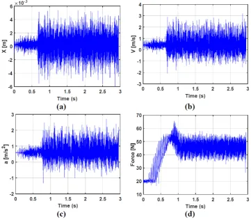
For real-time estimation of the structural pa -rameters of the system, the velocity and displace-ment signals are needed which are not directly available and are determined by integration of the tool acceleration collected by the accelerometer. In Figure 4, the acceleration and the resulting velocity and displacement signals along with the cutting force gathered by the dynamometer are shown for a sample test.
After gathering and determining y, ẏ , ÿ and F, their wavelet coefficients are calculated and by putting them in Eq. (12) and solving it, m,
Fig. 3. The test setup showing the accelerometer, the dynamometer, the tool and the nozzle of the lubricant
Fig. 4. The collected and estimated signals. W = 1800 rpm, depth of cut = 0.5 mm. (a): displacement;
For the validation of the extracted structural parameters, the lob diagram of each test is plot-ted based on the estimaplot-ted parameters, and it is investigated that whether it can correctly estimate the stability status of the operation. In Figure 5, the achieved lobe diagrams are depicted for three sample operations.
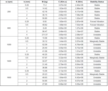
According to Table 1, the operation with the spindle speed of 200 rpm and depth of cut of 0.5
mm is stable. Moreover, it can be seen that the lobe diagram shown in Fig. 5-(a) which is ex -tracted based on the estimated structural param-eters of this operation confirms it too, showing that the system identification algorithm works correctly. Similarly, for two other operations in-dicated in Figs. 5-(b) and (c), the algorithm has succeeded in predicting true structural parame-ters because the lobe diagrams truly estimate the
Table 1. The estimated values of the structural parameters
w (rpm) b (mm) M (kg) C (N/m.s) K (N/m) Stability Status
200
0.25 11.2 3.07e+02 2.40e+06 Stable
0.5 14.42 1.63e+03 2.96e+06 Stable
1 42.16 3.92e+03 8.17e+06 Stable
2 36.15 2.66e+03 7.08e+06 Stable
4 50.80 4.31e+03 1.22e+07 Stable
600
0.25 6.92 1.60e+03 2.87e+06 Forced Vibration
0.5 48.62 1.69e+03 7.53e+06 Forced Vibration
1 6.49 6.80e+00 1.27e+06 Stable
2 56.47 3.46e+03 1.19e+07 Stable
4 211.07 3.85e+03 2.08e+07 Unstable
1000
0.25 15.56 1.09e+03 3.62e+06 Stable
0.5 35.12 1.44e+03 5.57e+06 Marginally Stable
1 52.09 1.41e+03 6.76e+06 Unstable
2 25.40 3.55e+03 8.73e+06 Unstable
4 41.06 3.05e+03 1.01e+07 Unstable
1400
0.25 40.25 4.81e+02 3.63e+06 Stable
0.5 57.67 3.32e+03 5.08e+06 Marginally Stable
1 34.07 1.61e+03 6.64e+06 Unstable
2 31.49 2.79e+03 8.64e+06 Unstable
4 36.88 4.51e+03 9.21e+06 Unstable
1800
0.25 15.48 2.13e+03 3.52e+06 Stable
0.5 20.23 1.50e+03 5.34e+06 Marginally Stable
1 49.93 1.64e+03 6.42e+06 Unstable
2 54.85 2.27e+03 8.07e+06 Unstable
4 27.85 6.66e+02 5.05e+06 Unstable
status of these processes. The operations in Figs. 5-(b) and (c) are respectively marginally stable and unstable.
Model Predictive Control
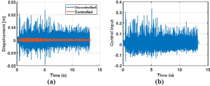
After obtaining m, c, and k, the unstable operations should be controlled. The results of applying MPC on two different unstable turning processes are depicted in Figs. 6 and 7. In these figures, the displacement of the tool when there is no control algorithm and when the control algorithm is on are presented. In addition, the control effort is shown for each process. As it can be seen, the range of the displacement of the tool when there is no control algorithm is high, because the operation is in the chatter mode. On the other hand, according to Figs 6-(a) and 7-(a), after applying MPC algorithm, magnitude of the tool displacement is decreased signifi -cantly which demonstrates that MPC can effec
-tively curb the unwanted vibrations of the tool. Another important point is that, the time needed for MPC algorithm to stable the process is very short and in other word, the rise and settling time is acceptable in this control algorithm. It has this advantage that before adverse influences of chat -ter can affect the workpiece and machine-tool, the MPC will act and force the unstable process to the stable zone.
Furthermore, the control efforts are shown in Figs. 6-(b) and 7-(b). From these figures, it is clear that the control energy needed for controlling the process is very low. This low control energy can be easily applied by the actuators such as tuned-mass-dampers, repre-senting another important pro of MPC. Since, actuators usually have limitations on the en-ergy that they can apply to the system. Usu-ally, very low and very high inputs can not be applied by the actuators to the system, unless very expensive ones.
Fig. 6. The results of applying MPC. (a): The comparison between the output of the system when the control
algorithm is not working and is working. (b): The control effort. w = 600 rpm, depth of cut = 4 mm
Fig. 7. The results of applying MPC. (a): The comparison between the output of the system when the control
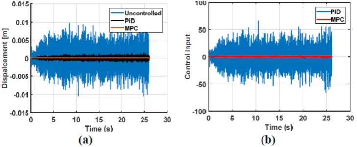
For more investigation of the MPC algorithm, the performance of the MPC and PID are com-pared in Figs. 8 and 9. From Figs. 8-(a) and 9-(a), it is clear that the MPC can limit the unwanted vi-brations of chatter more effectively than PID. For instance, in Fig. 8-(a), the maximum displace -ment of the tool after applying MPC is 0.44 mm while this parameter is 2.58 mm for PID. Also, maximum magnitude of the tool displacement is 0.003 mm for MPC and 1.61 mm for PID, for the process shown in Fig. 9-(a). Additionally, the control effort of MPC as it is shown in Fig. 8-(b), is between 2.12 and -2.00, whereas for the PID is in the range of 45.94 and -39.38. This parameter for the process depicted in Fig. 9 is between 66.50 and -64.87 for PID whereas 0.03 and -0.02 for MPC. Therefore, it can be concluded that MPC can effectively bound the unstable vibrations of tool while its control input is much lower than PID, showing the great strength and effectiveness of MPC in comparison with PID algorithm.
CONCLUSION
Regenerative chatter is a common phenome-non in machining process and has many destruc-tive effects on the machine-tool and workpiece. Therefore, for preventing its adverse conse-quences, it is vital to control the process online. For the purpose of system control, the structural parameters of the system are needed first, while they are not usually available since some pre-tests such as the impact hammer test should be implemented which is not practical especially in working environments. In this work, the aim was predicting the structural parameters of the sys-tem online and control of the process based on the achieved parameters. To do this, for system identification, the wavelet coefficients of the dis -placement, velocity, acceleration, and force sig-nals are calculated and then by substituting them in the system equation of motion and solving it, the structural parameters are achieved. Then, for
Fig. 8. The results of applying two control algorithms of PID and MPC. (a): The comparison of the tool
displace-ment; (b): The comparison of the control effort. w = 1400 rpm, depth of cut = 2 mm
Fig. 9. The results of applying two control algorithms of PID and MPC. (a): The comparison of the tool
the purpose of validation, the lobe diagrams of processes are extracted based on the estimated parameters and it is seen that they can correctly estimate the stability status of each process. Af-ter identifying systems parameAf-ters, the unstable turning processes are controlled by the MPC al-gorithm. For investigation of MPC performance, MPC and PID algorithms are compared. The re-sults indicate that MPC can control the process very more accurately than PID and in the same time the control effort of MPC is much lower than PID controller which shows the superiority of the MPC over PID. Online system identifica -tion without needing any previous informa-tion, controlling the chatter phenomenon via MPC which has low delay, high performance along with low control effort are the main features of the presented method.
REFERENCES
1. Altintas, Y. and M. Weck, Chatter stability of metal cutting and grinding. CIRP annals, 2004. 53(2): 619-642.
2. Lu, K., et al., Model-based chatter stability
pre-diction and detection for the turning of a flexible
workpiece. Mechanical Systems and Signal Pro-cessing, 2018. 100: 814-826.
3. Eynian, M. and Y. Altintas, Chatter stability of general turning operations with process damping. Journal of Manufacturing Science and Engineer-ing, 2009. 131(4): 041005.
4. Turkes, E., et al., Linear analysis of chatter vibra-tion and stability for orthogonal cutting in turning. International Journal of Refractory Metals and Hard Materials, 2011. 29(2): 163-169.
5. Schmitz, T.-K.S., Machining Dynamics Frequency
Response to Improved Productivity Springer
Sci-ence+ Business Media. 2009, LLC.
6. Liu, Y., et al., Chatter reliability prediction of turning process system with uncertainties. Me-chanical Systems and Signal Processing, 2016. 66: 232-247.
7. Den Hartog, J.P., Mechanical vibrations. 1985: Courier Corporation.
8. Lin, S. and M. Hu, Low vibration control system in turning. International Journal of Machine Tools and Manufacture, 1992. 32(5): 629-640.
9. Frumusanu, G.R., et al., Development of a stability
intelligent control system for turning. The Interna-tional Journal of Advanced Manufacturing Tech-nology, 2013. 64(5-8): 643-657.
10. dos Santos, R.G. and R.T. Coelho, A contribu-tion to improve the accuracy of chatter prediccontribu-tion in machine tools using the stability lobe diagram. Journal of Manufacturing Science and Engineer-ing, 2014. 136(2): 021005.
11. Kurata, Y., et al., Chatter stability in turning and
milling with in process identified process damping.
Journal of Advanced Mechanical Design, Systems, and Manufacturing, 2010. 4(6): 1107-1118. 12. Chun-Lin, L., A tutorial of the wavelet transform.
NTUEE, Taiwan, 2010.
13. Huang, S., G. Qi, and J. Yang. Wavelet for system
identification. in Proceedings-Spie The Interna
-tional Society For Optical Engineering. 1994. Spie International Society For Optical.
14. Wang, L., Model predictive control system de-sign and implementation using MATLAB®. 2009: Springer Science & Business Media.
![Fig. 1. One DoF mass-spring-damper model of the turning process [4]](https://thumb-us.123doks.com/thumbv2/123dok_us/8805325.1774259/3.595.71.287.610.736/fig-dof-mass-spring-damper-model-turning-process.webp)