A Framework for Provisioning Availability of NFV
in Data Center Networks
Jingyuan Fan, Meiling Jiang, Ori Rottenstreich, Yangming Zhao, Tong Guan, Ram Ramesh, Sanjukta Das and
Chunming Qiao,
Fellow, IEEE
Abstract—Network Function Virtualization (NFV) is a promis-ing technique to greatly improve the effectiveness and flexibility of network services through a process named Service Function Chain (SFC) mapping, with which network functions are de-ployed over virtualized and shared platforms in data centers. However, failures are quite common in data centers. Therefore, a practical and yet theoretically challenging issue in SFC mapping in such an environment is to manage the availability of the requests.
In this paper, we present a framework to provision availability of SFC requests in a data center with multiple layers of connected devices, and the devices follow heterogeneous failure processes with the objective of minimizing resource usage. To expedite the process, we further propose an optimization problem of request mapping and backup estimation, and solve it efficiently with an approximation algorithm. With simulations, we demonstrate the effectiveness of our proposed framework.
Index Terms—Data centers availability, Network function vir-tualization, Service function chaining
I. INTRODUCTION
A
S an advanced application of virtualization technologies, Network Function Virtualization (NFV) eliminates the need for dedicated middleboxes and enables the allocation of computing and networking resources in a flexible manner. In the NFV environment, traditional hardware-based network appliances are replaced by software-based virtual network functions (VNFs), which implement network functions in software. These VNFs are deployed on virtual platforms where clients (each associated with a sequence (chain) of required funcions) may share the same physical hardware through a process named Service Function Chain (SFC) mapping.However, one of the most important issues of a successful NFV deployment is to manage the availability of the requests. Compared to traditional IT application with availability of the order of two 9s to three 9s (i.e., 99% and 99.9% of the time), telecom service requires their network being “always on” (i.e., five 9s or six 9s of the time [23]).
Manuscript received May 3, 2018; revised August 19, 2018. This work was supported in part by NSF grant EFMA 1441284.(Corresponding author: Yangming Zhao.)
J. Fan, Y. Zhao, T. Guan and C. Qiao are with the Department of Computer Science and Engineering, University at Buffalo, The State Uni-versity of New York, Buffalo, NY 14260 USA (e-mail: [email protected]; [email protected]; [email protected]; [email protected]).
M. Jiang, R. Ramesh, S. Das are with the Department of Manage-ment Science and Systems, University at Buffalo, The State University of New York, Buffalo, NY 14260 USA (e-mail: [email protected]; [email protected]; [email protected]).
[image:1.612.324.548.191.266.2]O. Rottenstreich is with the Technion - Israel Institute of Technology, Haifa, 3200003, Israel (e-mail: [email protected]).
Fig. 1. Alternating renewal process
Managing availability, in practice however, is not easy. The challenge is multifold: 1) a data center, which holds VNFs, includes connected devices, such as servers, switches and links, each having multiple layers (e.g., software and hardware), and can have various topologies; 2) device failures are quite common and the failure and repair processes of each device in a data center can experience heterogeneous probability distributions; 3) failures of different devices can have different influences on service availability, e.g., a virtual machine (VM) vs. a core switch; 4) the availability of an SFC request can vary with its location in the data center; 5) redundancy may need to be provisioned in order to meet the availability requirement; 6) determining the optimal amount of backup resources in such a dynamic data center environment, which is important to reduce resource consumption, makes the problem even harder. Therefore, there is a need for a framework to easily estimate the availability of SFC requests as well as to allocate the minimum amount of resources needed to meet heterogeneous availability requirements, for any given data center topology with heterogeneous failure and repair processes of each device.
Despite the importance of provisioning availability in NFV, few solutions have been suggested. In [17, 18] the authors proposed online algorithms for availability guarantee with on and off-site backups. However, they did not consider the heterogeneous processes of a device’s failure and repair, and they assumed that only VMs would experience failures and ignore others, such as switches and links, which also have been identified as a major contributing factor to downtime [19]. On the other hand, [45] provided a framework to evaluate fault-tolerance in user-defined data center topologies while considering various types of devices, but a mechanism to guarantee availability was not described.
2
Fig. 2. Case study: a 4-ary Fat-tree data center topology [4]
We focus on the case where SFC requests are implemented with the widely used consolidated middlebox structure [5, 20, 46], in which each VNF is an application that can be realized with certain number of VMs installed on the physical machines and an entire service chain running as a native process at a single physical machine [24, 27, 41, 48]. To the best of our knowledge, none of the existing works have addressed similar problems. Specifically, when a request comes, we map it to the data center, evaluate its availability and provision backups until its requirement is met. To this end, we first show a mechanism to calculate the downtime of an SFC request in such an environment via a Markov Chain Monte Carlo (MCMC) like procedure. Even though this method is very accurate, it suffers from low efficiency [28, 51]. Such problem is further exacerbated by the iterative nature of our algorithm. To address the challenge, we propose an optimization problem that estimates the number of backups required and aims at minimizing the resource usage upon the arrival of a request, while considering both request placement and backup provisioning, thereby significantly reducing the number of iterations needed of our framework. To efficiently solve the optimization problem, we propose an approximation algorithm with a lower bound on the availability that can be achieved. The performance of our framework is validated through simulations.
In summary, our contribution is multifold: 1) to the best our knowledge, no work has considered the end-to-end availability problem with each devices state modeled as an alternating renewal process. Such a model is closer to reality, but consider-ing it makes our problem significantly harder; 2) to resolve the complexity, we proposed an optimization problem to estimate the number of backups needed while reducing the resource usage; 3) we gave an approximation algorithm to solve the problem.
The rest of the paper is organized as follows. Section II describes the availability model of a single device as well as VNFs used in the paper. In Section III, we describe the overall structure and design of our proposed framework and show how it works with a case study. Section IV defines the problem of request mapping and backup estimation in NFV, which is part of the framework, and presents an algorithm with a theoretical bound on the availability that can be achieved. We evaluate its performance in Section V, survey related work in Section VI and briefly discuss the usage issues of our framework and
future works in Section VII, followed by conclusions VIII.
II. AVAILABILITYMODEL
A. Availability Model of A Single Device
The availability of a component is often considered as the relative share of time the component is functioning, and thus the probability to find the component working if checking it at a random point in time. Therefore, existing works [16, 17] considering availability assume that the availability of a device can be calculated using uptime followed by downtime:
A= U ptime
U ptime+Downtime =
M T BF
M T BF+M T T R (1)
where MTBF and MTTR areMean Time Between Failureand
Mean Time To Repair, respectively.
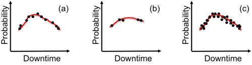
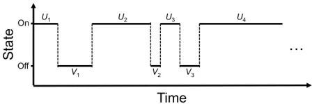
However, such model fails to capture the non-deterministic characteristics of devices in practice [6, 15]. To have a more accurate analysis, in this paper, we model a device’s failure as an alternating renewal process (ARP) [9], as shown in Fig. 1. An ARP models a system that alternates between two states (onandoff) over time. W = ((U1, V1),(U2, V2), . . .) are the
pairs of times successively spent in the two states, where the sequence U = (U1, U2, . . .) and V = (V1, V2, . . .) are the
successive lengths of time that the system is in stateonandoff, respectively and both of them are assumed to be independent and identically distributed random variables. In other words, the system starts in state on and remains in that state for a period of timeU1, then goes to stateoffand stays in this state
for a period of time V1, then back to stateonfor a period of
time U2, and so forth. With such a model, even computing
availability becomes a hard problem, which will be described and addressed in the next section.
B. Availability Model of Consolidated Middleboxes
Algorithm 1The framework for provisioning availability for the requestr
1: Map the requestrwith an availability requirementαronto
the network 2: whiletrue do
3: if CALCULATE AVAILABILITY(r)< αr then
4: Provision backups to the requestr 5: ifthere is not enough resource then
6: break
7: else
8: Go to the next request
time to transfer states for stateful VNFs, is zero, and will extend our analysis in a future work.
Therefore, given an SFC with M VNFs, each of which requires n1, n2, . . . , nM VMs respectively, we consider the
service as available if 1) the i-th VNF should have at least ni VMs available, where i = 1,2, . . . , M, and the physical
machine holding these VMs is available; 2) there should be at least one available path (including links and switches/routers along the links) between the physical machine and any one of the access switches (the highest level switches) of the data center.
As we consider a consolidated middlebox model in this work, the availability of an SFC can be bounded by the avail-ability of the physical machines where the VMs implementing the SFC reside. The failure of the physical machine can result in a violation of the availability requirement no matter how many backup VMs are allocated on it. For example, as shown in Fig. 2, even though a datacenter network is by design toler-ant to failures of switches and links, with resource redundancy that contribute to the multi-path connections between a server (e.g., s11) and the highest level switches (as shown by the
dashed lines), it may still not be enough to achieve certain availability requirements. In other words, the probability that there is at least one path available froms11 to any one of the
core switches is already lower than the required one. Thus, VMs should also be allocated at physical machines besides the primary one; and therefore, the number of VMs allocated at a secondary physical machine should be at least PMi=1ni,
and multiple secondary physical machines may be required. When there are multiple physical machines used, at least one of them should satisfy the conditions aforementioned for this service to be available.
C. Assumptions
[image:3.612.315.565.60.125.2]In this paper, we assume that the failure and repair processes of each and every device (including physical machines, VMs, routers, switches, etc.) is modeled by an ARP with heteroge-neous U andV sequences, and the distributions from which each ARP’sU andV are drawn are stationary. In this work, we assume that only VMs (i.e., VNFs) have backups and there is no correlated failure between devices and the failure of each device is independent for simplicity.
Fig. 3. Maximum likelihood estimation of the downtime distribution with: (a) an appropriate sample size; (b) undersampling; (c) oversampling. The X-axis is downtime and the Y-axis is probability.
III. FRAMEWORK FOR PROVISIONING AVAILABILITY
A. Overview
As provisioning availability of an SFC request with the failure probability of each device being a constant is already an NP-hard problem [16], using an ARP model for evaluating availability further increases the complexity, and analysis on how to guarantee availability in the existing works [16, 17] cannot be applied directly.
To address the problem, we apply an iterative approach to increase the availability of an SFC request by provisioning backups until either the availability requirement is met or no more resource is available, as shown in Algorithm 1. Specifically, given the topology of a data center as well as the failure and repair probability distributions of each device, and an SFC request r with availability requirement αr, the
framework will first map the request onto the topology (line 1, see more details in Section IV), calculate its availability (function CALCULATE AVAILABILITY(r) of line 3). If the availability of the request cannot meet the user’s requirement, it will provision some backups (line 5) to the request and repeat the above process.
As in [45], a data center topology can be described as an abstract tree with a root node, where if a father node fails, all its children cannot be reached via this father node. Some nodes can have multiple layers of failures and they may have different influences. For example, a switch can contain multiple ports. The failure of a switch can be seen as the failure of the whole switching fabric and consequently none of the devices connected to the switch are reachable from the switch, while the failure of a port does not affect the devices connected to other ports of the switch.
For the rest of the section, we will focus on how to calculate the availability in Section III-B (line 6), and how to add backups in Section III-C (line 8), while leaving request mapping to the next section.
B. Calculating Availability for SFC Requests
To estimate the availability of a mapped request over its contract period duration, the main idea is to sample the potential states (on/off) of each component that may fail at different time intervals.
4
Switch
Switch
Server
VM
1
t =Δt
1
…
…
t =Δt t = 2Δt t = nΔt
(a) Mapping an SFC request
Switch
Switch
Server
VM
1
t =Δt
1
…
…
t =Δt t = 2Δt t = nΔt
(b) Estimating downtime distribution of a mapped SFC request
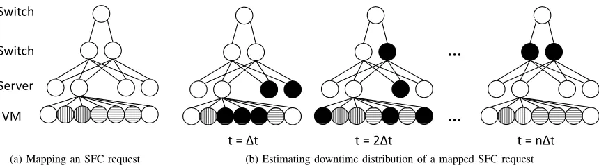
Fig. 4. A toy example of how to estimate availability of a mapped SFC request (circles filled with vertical and horizontal lines represent VMs belonging to two different requests; black circle means the device is unavailable)
on the state at time(n−1)∆t. Therefore, we can emulate the state transition of each device by sampling its corresponding failure and repair probability distributions at each time slot.
Then at each time slot, the breadth-first search (BFS) algorithm is used to see how many physical machines used for an SFC request we can “reach” from the top of the constructed abstract tree. Here a reachable physical machine means all components on at least one path from the top of the tree to this physical machine are inonstate. For a reachable physical machine, if any one of the VNFs of this SFC request does not have the required number of VMs, we consider this physical machine as being down at this time slot for this request. If all reachable physical machines are down, we consider this time slot as downtime for this request.
By running the above BFST consecutive times and count-ing the number of time slots that are down for the request, we can obtain the total downtime during the time interval [0, T], which can be considered as one sample from the unknown downtime distribution. Then we repeat the above procedure for N times (so that we have N samples), and calculate the frequency of each downtime that occurs in our samples S, where|S|=N:
PM LE(X =s) =
COUNT(s)
N , s∈S (2) which equals the maximum likelihood estimation (MLE) of the downtime distribution of the request. Then we apply kernel density estimation (KDE) [42] to generate the probability density function (PDF) of f of the downtime, as shown in Fig. 3(a). Thus the availability can be estimated as1−R∞
0 fdt.
A toy example is shown in Fig. 4. An SFC request with two VNFs, each of which requires 1 and 2 VMs indicated by vertical and horizontal lines (the rest can be considered as backups) respectively, is mapped on a data center with two layers of switches, as shown in Fig. 4a. Fig. 4b depicts the procedure of estimating its availability. A black circle indicates the device being unavailable at that time slot. Att= ∆t, the number of available VMs is less than the requirement; while at t=n∆t, the VMs are not reachable from the top switch even there are enough available VMs. Therefore, the service should be considered as unavailable during these two time slots. On the other hand, at t = 2∆t, the service is available as both conditions discussed in Section II-B can be met. Clearly with more backup VMs and physical machines, the chance that a mapped request can meet its availability requirement is higher.
In order to get the downtime distribution estimation, we first need to understand how many samples are needed. The estimated distribution cannot converge if it is under sampled (Fig. 3(b)), but oversampling (Fig. 3(c)) can lead to too much computational overhead. To this end, we empirically evaluate this by setting a relatively large initial sample size, taking progressively larger sample sizes (e.g., 1000 more each time), and deriving the estimated PDF for each until the difference between the estimated downtime distribution and the reference one, which can be acquired by evaluation with a very large sample size, is smaller than , where is a small number. The difference between two distributions can be measured in various ways, such as Kolmogorov-Smirnov test [11], and Kullback-Leibler divergence [32]. Note that simply comparing the estimated availability (i.e., the integral of the estimated downtime distribution) is not good enough as a small sample size may result in a similar expected availability to the reference one while a distribution looks quite different.
Algorithm 2 Provisioning backups 1: Initialize:
2: nmin = min (nr1,. . .,n r Mr) 3: unit= hb nr1
nminc,b
nr2
nminc, . . . ,b
nrM nminc
i
4: backup= [0,0, . . . ,0]
5: times= 1
6: function ADD BACKUPS(r)
7: ifbackupi≥ uniti×times ∀i∈[1, Mr] then
8: times++
9: fori= 1 toMr do
10: if backupi <times ×uniti then
11: backupi =backupi + 1
12: returnbackup
C. Provisioning backups
If the estimated availability is smaller than the required one, backups are provisioned. Meantime, we want to minimize the number of backups allocated to 1) save resources for other requests; and 2) reduce costs. Assume an SFC request rthat needs Mr VNFs, each of which requires hnr1, n
r
2, . . . , n
r Mri
VMs respectively, is given. We use Algorithm 2 to allocate backups (line 8 in Algorithm 1). Each time a backup needs to be provisioned, the function ADD BACKUPS is called. For ease of presentation, we denotehnr
[image:4.612.93.523.55.174.2]The key idea of the algorithm is trying to ensure that the number of backups allocated for the i-th VNF is proportional to the number of VMs it initially requires (i.e., nr
i) while
keeping at most one backup VM allocated to each VNF each time. The intuition here is that if a VNF requires more VMs, more backups should be allocated as it has a higher chance to have at least one VM down while keeping the increase of VM usage to a minimum.
To this end, we build Algorithm 2 based on iterative water-filling algorithm [55]. First Vr is scaled down with the
scale factor mininri, denoted as unit, and it (multiplied
by times) is used as the “water level” for deciding if more backups should be allocated to a VNF with times increases as the “level” is evened. For example, assume that Vr =h10,3,7i, then nmin = 3 and unit=h3,1,2i. In this
case, times is increased every three times the function is called. When the function is called the first time, one backup is allocated to each of the VNF; one is allocated to the first and third VNFs respectively the next time the function is called; if the function is invoked again, one VM is provisioned to the first VNF. This loop continues if more backups are needed with increasing timesby one.
As mentioned in the previous section, the availability of an SFC is bounded by the availability of the physical machines that holds the VMs implementing this SFC. Thus sometimes multiple physical machines are needed for one request. To minimize the usage of physical machines, only when adding backups to a physical machine cannot increase the availability, we select a new physical machine, and allocatePMr
i=1nri VMs
on the new physical machine for the request. Backups, if still required, are only provisioned to this new physical machine until a new physical machine is added.
D. Case Study
In this subsection, we show how our framework works through an example. Consider an SFC request r and a 4-ary Fat-tree data center topology [4] as shown in Fig. 2. The request has an availability requirement of 99% for a contract period duration of 30 days. It requires 4 VNFs, each of which requires 3, 10, 21, 15 VMs, respectively. Note that our framework also works for other types of topologies, such as DCell [22] and BCube [21], which are recursively defined.
∆t is set to 1 minute, and a Gaussian kernel is applied for KDE. In this example, the request is mapped initially to a randomly selected physical machine in the network.
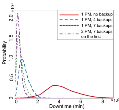
Fig. 5 presents how the availability improves with differ-ent number of backups through the changes in downtime distribution. At the very beginning, no backup (red line) is added to the request. Based on the distribution, the availability can be estimated as 0.902. When adding more backups, the availability keeps increasing (0.981 for blue line and 0.989 for green line) until achieving the availability requirement (0.992 for purple line). Note that after we add 7 backups to the request (green line), the availability cannot be further improved1 by
1More precisely, with 7 backups, the availability of this VNF is very close
[image:5.612.334.534.55.240.2]to the availability of the physical machine, which is the availability upper limit of the VNF.
Fig. 5. Downtime estimation with different number of backups (PM: physical machine)
adding more backups to the same physical machine (which is not shown in the figure); and therefore, we add one more physical machine with 49 VMs (0 backup VM), re-estimate the availability and get the purple line. When there are two physical machines, a time slot is count as uptime if at least one of the machines has at least 49 VMs and that machine is reachable from one of the core switches. In this study, the sample size |S| is at least 4,000 for the estimated downtime distribution to converge. In general, we find that the sample size needs to be quite large.
E. Increasing Estimation Efficiency
One drawback of the above method is the extremely low efficiency. The total running time of a naive implementation of a solution for the example in the previous subsection, written in non-optimized Python code, takes more than 1,100 hours on a Linux machine with 3.60GHz Intel i7-4790 cores and 12GB memory. To improve the computational efficiency, we made a few optimizations to our implementation:
Mapping requests with selected physical machines. Since the availability that an SFC achieves is bounded by the avail-ability of the physical machines implementing this SFC, we can always choose physical machines with higher availability to implement SFC requests with stricter requirement. To this end, we define thepath availability of a physical machine as the probability that all components of at least one path from the top of the hierarchy network to this physical machine are up. Take the upside down tree shown by dashed lines in Fig. 2 as an example, we should have the servers11 to be available,
the edge switch e5 to be available and at least one the two
options: 1)a4 is available together with at least one of c0 or
c1; or 2)a5 is available together with at least one ofc2or c3.
6
be calculated as
G(s11) =αs11×αe5×(1−(1−αθ1)×(1−αθ2))where
αθ1 =αa4×(1−(1−αc0)×(1−αc1))
αθ2 =αa5×(1−(1−αc2)×(1−αc3))
(3) where αd is the availability of device d. Note that in this
example, we just consider the failures of switch and server, but one can extend it to include links, ports, etc. With the path availability, one can estimate how many physical machines are needed at least.
Pruning the search space. Consider the same example. Assume that an SFC request is mapped to the physical machine s11, then instead of including all nodes in the abstract tree in
the search space, only searching over nodes that are used in calculating its path availability are necessary and sufficient. In our case, these nodes are s11, e5, a4, a5, c0, c1, c2, and
c3. With a data center topology with a very large number
of switches and physical machines, eliminating unnecessary nodes in the search space can lead to a significant performance improvement.
Parallelizing the search. Clearly, the BFS algorithm can be easily parallelized and/or distributed. Each core can run fewer iterations, and all the samples can be merged together at last to get the estimation. By default, all available cores are used by our framework.
With parallelism and the other two optimizations, we run the same experiments as the one in the case study on Dell PowerEdge R720 with Intel Xeon E5-2600 cores and 128 GB memory. It took around 40 hours on 40 non-dedicated cores. The computational efficiency can be further improved with more cores/machines.
However, even though the efficiency is greatly improved, our framework is still not ideal in the sense that the process can be further prolonged with 1) an even higher availability requirement, which is normal in a carrier-class network [23] (usually requires an availability of 99.999% or 99.9999% (five 9s or six 9s)) and 2) longer contract period duration. A question arises naturally: can we further reduce the running time?
IV. OPTIMIZINGAVAILABILITYPROVISIONING INNFV To answer the question raised in the previous section, we first need to understand what are the major contributing fac-tors. Recall that in order to estimate the downtime distribution, we need to run simulations similar to MCMC [51], and for the estimated downtime distributed to converge, a large sample size is needed. Such procedure, in spite of being accurate, is time consuming by nature [28]. Even with a much simpler model, the work in [45] still requires a long time to evaluate availability/reliability. In addition, iterations are needed to improve availability to meet requirements.
Fortunately, there is still room to alleviate the situation and our insight here is that if we can accurately estimate the number of backups that each request needs, instead of just mapping the required VMs when a request arrives, we can map them together with backups (line 1 in Algorithm 1). Therefore, when we evaluate the availability (line 6 in
Algorithm 1), a mapped request can have an availability very close to its requirement, thereby reducing the total running time. In this section, we will model the request mapping and backup provisioning as an optimization problem with the objective of minimizing the total amount of resources usage and show an approximation algorithm to efficiently solve it.
A. How to Deal with Heterogeneous Failure Processes of Devices?
The first problem to deal with is the heterogeneous failure processes, which are modeled as alternating renewal processes, of devices. Letµ=E(W)denote the mean of a time period that the device is on and ν = E(U) denote the mean of a time period that the device isoff. Letp(t) =P[device is on] be the probability that the device is on at time t ∈ [0,∞). Since the uptime (downtime) of a device is non-arithmetic, we have the following two relationships by the alternating renewal theorem [56]:
lim
t→∞P[device ison att] = µ µ+ν
lim
t→∞P[device isoffatt] = ν µ+ν
(4)
Thus, as ∆t is very small compared to the contract period duration, we approximate each device’s state as a Bernoulli variable with the success probabilityp=µµ+ν.
B. Computing Availability of SFCs
An SFC request r is defined as a tuple r = hαr, Vr, trstart, trend, b
ri, where α
r is the availability
require-ment, Vr = hnr1, nr2, . . . , nrMri is the minimum number of
VMs required of each VNFs for the service to be available. tr
start andtrendspecify the contract start and end time,
respec-tively. br is the bandwidth requirement. Here we assume the
egress and ingress traffic are the same, and since we assume a consolidated middlebox structure, the traffic between VNFs is ignored.
Given such an SFC request r, and assume that
hkr
1, k2r, . . . , kMrri backups are allocated, the probability that
thei-th VNF is available is:
P[i-th VNF is available] =Pnr i+kri[X
r
i ≥nri] (5)
where Xr
i is a variable indicating the number of available
VMs. Since the VMs’ states are modeled as independent Bernoulli variables with different success probability, the sum of these variables, denoted asNr, follows a Poisson binomial
distribution [13]. Letξr
k=P[Nir=kr],kr= 0,1, . . . , nri+kir
be the probability mass function (PMF) for the Poisson bi-nomial random variable Nr
i, then the cumulative distribution
function (CDF) of Nir, denoted byFNr i(k
r) =
P[Nir ≤k r],
kr= 0,1, . . . , nri+kri, gives the probability of having at most krsuccesses out of a total ofnri+kri, and can be written [53] as:
FNr i(k
r) = kr X
m=0
ξmr = kr X
m=0
X
A∈Rm Y
j∈A pj
Y
j∈Ac
(1−pj)
TABLE I
SYMBOLS AND THEIR DEFINITIONS
Symbol Definition
tr
start The start time of ther-th request tr
end The end time of ther-th request nr
i The required number of VMs of thei-th VNF of ther-th request αr The availability requirement of ther-th requirement Mr The total number of VNFs of ther-th request FNr
ij(x) The probability of having at mostxVMs are available of all VMs mapped to thej-th physical machine
Rm The set of all subsets ofmVMs of all VMs
whereRm is the set of all subsets of mintegers that can be
selected from{1,2, . . . , nri+kri}, andAcis the complement of
setA. Note that when allpj are identical, the above equation
is just the CDF of a Binomial distribution. Therefore, we have
Pnr i+kir[X
r
i ≥n
r
i] = 1−FNr i(n
r
i −1). (7)
Thus, the probability that all the VNFs are available can be expressed as
Mr Y
i=1 Pnr
i+kri[X r
i ≥n
r i] =
Mr Y
i=1
1−FNr i(n
r
i −1)
. (8)
However, computing such a function is not easy, which requires one to enumerate all elements inRm, which requires
to consider an exponential number of scenarios. It is very large even whennri+kiris small. In general, we show the following theorem:
Theorem 1. Verifying if the availability of a given deployed SFC request with backups is above a given threshold is PP-complete.
Proof. Rewrite Eq. (6) as a boolean formula, where xj and ¯
xj represent if thej-th VM is available or not, whileQand Pare replaced by∧and∨, respectively. By the definition of
language in PP, it is clear this problem is in PP. To show PP-completeness, we can reduce MAJSAT problem [33] to this problem. MAJSAT is a decision problem where one needs to decide if half of all assignments can satisfy a given Boolean formula, and it is PP-complete. Note that, for an instance φ with n variables of MAJSAT, the number of all possible assignments to φis2n. Thus, we have
φ∈M AJ SAT ⇐⇒the number of assignments that
satisfies φis greater than 2n−1
⇐⇒Pr[φ(x)]> 1
2 withx∈ {0,1} n
Given that the instance of this problem is a pair (φ, θ)
consisting of a Boolean formula φ and a thresholdθ. Hence, with a MAJSAT instance φ, we can set instance (φ,1/2) for this problem. To verify the correctness,
φ∈M AJ SAT ⇐⇒Pr[φ(x)]> 1
2 withx∈ {0,1} n
⇐⇒the probability that φcan be satisfied
> the given threshold 1 2
⇐⇒(φ,1
2)∈this problem,
Thus, it is a valid many-one reduction from MAJSAT problem to this problem. Therefore, our problem is also PP-complete.
To efficiently compute the availability of an SFC if only one physical machine is used, we adopt [26]. Interested readers can refer to the paper for more details. When multiple physical machines are used, the availability is the probability that at least one of the physical machines as well as all the VNFs deployed on the physical machine is available.
C. Problem Formulation
In this subsection, we formulate the request mapping and backup provisioning problem as an integer program. For ease of reading, Table I provides a list of symbols defined in previous sections.
As mentioned, the data center topology can be described as an abstract tree with Nsphysical machines (i.e., nodes on
the second layer from the bottom), and each physical machine j ∈ [1, Ns] can contain up to cj VMs. We are also givenR
SFC requests.
To formulate the problem, two binary variables are defined. xr
j = 1 if the r-th request uses VMs of the j-th physical
machine; otherwise, xr
j = 0. Likewise, yjkrt equals 1 if the
r-th request uses r-the k-th VM of thej-th physical machines at time slott, wheretr
start≤t≤trendand1≤k≤cj; otherwise
yrt
jk= 0. Therefore, we can have the following constraints: X
r
yrtjk≤1 (9)
which means that at any time slot, at most one SFC request can use thek-th VM of thej-th physical machine. It also ensures that the maximum number of VMs of any physical machine that are used at any time slot is less than the capacity of the physical machine. Thus
xrj
Mr X
i=1
nri
!
≤X
k
yrtjk≤2×xrj
Mr X
i=1
nri
!
(10)
which guarantees that if r-th request uses VMs of the j-th physical machines (i.e.,xr
j= 1), at least PMr
i=1n
r
i VMs are
al-located at this physical machine for this request (Section II-B); otherwise, it should be zero, bounded by the left and right hand sides of the equation. The right hand side of the constraint sets the upper bound on the number of the backups to bePMr
i=1nri,
8
between a physical machine to a core switch, when mapping a request, we also need to reserve bandwidth resource on the selected paths between the physical machine that implements the request and any of the core switches. Accordingly, G(·)
should only include those selected paths.
Last but not least, the availability of an SFC request should always be greater than or equal to its requirement during the contract period duration:
1−Y j 1− Mr Y i=1
1−FNr ij(n
r
i −1)
×G(j)
!
xj !
≥αr
(11) where 1−FNr
ij(n r
i −1) = Pnr
i+kri[X r
i ≥ n
r
i] and the r-th
request is mapped to the j-th server.FNr
ij(·)is defined as in
Eq. (6). A VMe∈ Rm if and only ifyrtje= 1. To show this
in the formulation, we can rewrite the availabilitypk of a VM
k as pkyrtjk.
The objective of the problem is to minimize a weighted-sum of the number of VMs and physical machines that are needed:
ρX r X j X k
yjkrt+ (1−ρ) X
j
1 X
r
xrj ≥1 !
(12)
where0 ≤ρ≤1 is of one’s choice and1(·) is the indicator function. A higher value of ρ puts more emphasis on the number of VMs, e.g., when one tries to decide how much to charge users as with the current VM pricing models [1]; while a lower one puts more emphasis on the number of physical machines that need to be used, e.g., when energy consumption is more of a concern as we try to pack VMs into fewer physical machines and put the rest into hibernation [37].
D. Algorithm Design and Analysis
In this subsection, we propose an online algorithm to provision availability while mapping requests. Based on our complexity analysis above, we know that finding the optimal solution is challenging. Hence, to address the challenges, we decompose the problem into two phases: request mapping and backup provisioning. In request mapping, we need to select the physical machines to hold the request and reserve requested bandwidth from the machines to the core switches. In backup provisioning, we only consider the availability constraint in order to add backup VMs.
First recall the availability of a request when there is only one one used physical machine
Mr Y
i=1
1−FNr i(n
r
i −1)
(13)
As the availability requirement of an SFC request is usually very close to 1,FNr
ij(n r
i−1)should be close to 0. Therefore,
we can rewrite Eq. (13) as
Y
i
1−FNr ij(n
r
i −1)
= 1−X i
1−FNr ij(n
r
i −1)
+
X
w<v
1−FNr wj(n
r
w−1) 1−FNr
vj(n r
v−1)
−
X
w<v<u
1−FNr wj(n
r
w−1) 1−FNr
vj(n r
v−1)
1−FNr uj(n
r
u−1)
+. . .+ (−1)MrY i
FNr ij(n
r
i −1)
.
= 1−X i
FNr ij(n
r
i −1)
(14) Now, recall the definition of a supermodular function and a submodular function:
Definition 1. A functionf :X→Rissupermodulariff(x↑
y) +f(x↓y)≥f(x) +f(y),∀x, y∈X, wherex↑y denotes the component-wise maximum and x↓y the component-wise minimum of xand y.
Definition 2. If −f is supermodular, f issubmodular.
Therefore, we can have the following theorem:
Theorem 2. Fixing k, FN(k)is a decreasing supermodular function in the context of NFV and the decrement is propor-tional to the availability of the element added toRm.
Proof. We first prove the second half of the theorem and use the conclusion to prove the first half.
Given are two sets Rm = {1,2, . . . , n} and R0m = RmS{n+ 1}. LetFn(k)andFn+1(k)denote the probability
of having at mostkout of a total ofnandn+ 1, respectively. pi denotes the availability of thei-th component. Then
Fn+1(k) =
k X m=0 X A∈R0 m Y j∈A pj Y
j∈Ac
(1−pj)
=
(1−pn+1)
k X m=0 X A∈Rm Y j∈A pj Y
j∈Ac
(1−pj)
+
pn+1
k−1
X m=0 X A∈Rm Y j∈A pj Y
j∈Ac
(1−pj)
(15)
Therefore, we have
Fn+1(k)−Fn(k) =pn+1×
k−1
X m=0 X A∈Rm Y j∈A pj Y
j∈Ac
(1−pj)
−Fn(k)
=
−pn+1×
X A∈Rk Y j∈A pj Y
j∈Ac
(1−pj) =−pn+1ξk
(16)
where ξk is the probability of having k successes out of n.
As ξk > 0, we can see that fixing k, Fn(k) is a decreasing
function and the decrement is proportional topn+1.
Next, we show a sufficient condition forFn+1(k)−Fn(k)<
Fn+2(k)−Fn+1(k). To satisfy the inequality, we need
whereξ0kis the probability of havingksuccesses out ofn+ 1. By expanding bothξk andξ0k as summations, we can find that 2×ζ(ξk) =ζ(ξk0), whereζ(x)denotes the number of terms in
the summation form of x. To make them equal, rewrite each term ϕk inξk as 12 ×ϕk+12 ×ϕk. By subtracting the RHS
from the LHS of Eq. (17), we can have
pnξk−pn+1ξ0k= X Y
i∈B pi
Y
i∈C (1−pi)
1 2
Y
i∈D pi
Y
i∈E
(1−pi)− Y
i∈G pi
Y
i∈H (1−pi)
! (18)
where B,C,D,E ⊆ Rm and G,H ⊆ R0m, and furthermore, |E|<|H|, |D| ≥ |G| and|D|+|E|+ 1 =|G|+|H|. As in practice [3] (as well as our data from production data centers) the availability of a VM is quite high (at least greater than 0.9), Eq. (18) is greater than 0. Following a similar method, one can prove that FN(k)is a supermodular function.
If all physical machines for a request are selected, then we can rewrite Constraint (11) as
1−αr≥ Y
j 1−
Mr Y
i=1
1−FNr ij(n
r
i −1)
×G(j)
!!
(19) and takelog on both sides,
cr≥ X
j
log 1− Mr Y
i=1
1−FNr ij(n
r
i−1)
×G(j)
!!
(20) where cr = log(1−αr). Since
QMr
i=1
1−FNr ij(n
r
i −1)
×
G(j)≤1, the RHS of Eq. (20) can be approximated by Taylor series, and the availability constraint can be written as:
X
j
G(j) 1−X i
FNr ij(n
r
i −1)
!
≥c0r (21)
where c0r =−cr, as log(1−x) = −P ∞ n=1
xn
n <−x when
x≈0. Note that regardless of this relaxation, the solution is still valid and feasible asQMr
i=1
1−FNr
ij(n r
i −1)
×G(j)>
0.
Since the sum of supermodular functions is still supermod-ular, we know that Eq. (14) and the LHS of Eq. (21) is submodular. Therefore, we can have Algorithm 3.
The first step (line 1 to 3) is to pre-process the path availability for all Ns physical machines and sort all VMs
in each physical machines by their availability defined in Section IV-A in descending order. Clearly, there is a tradeoff: selecting all paths between a physical machine and all core switches would increase the path availability of the machine, but it also means that we need to reserve bandwidth for the SFC on all paths, which would waste a lot of resources. To this end, we set a tunable parameter K as the number of paths between the physical machines and all core switches that the algorithm considers. Besides, setting a smallKhelps to further prune the BFS search space and reduce the running time (Section III-B). In other words, a physical machine may have multiple path availabilities, each corresponding to a set of
Algorithm 3 GAP: Greedy availability provisioning in NFV 1: foreach physical machine j∈Ns do
2: Given the number of paths between the physical ma-chines and all core switchesK, compute all possible path availabilities
3: Sort VMs on physical machines by their availability (Section IV-A) in a descending order
4: foreach requestr∈Rdo 5: candidate=Ns
6: whiletrue do
7: Sort candidateby their available capacity and path availability in descending order and select the first M distinct physical machines asC
8: forphysical machinei∈C do 9: Map PMri=1nr
i VMs on each of the physical
machine and reserve bandwidth on corresponding paths
10: whileEq. (21) is not metdo
11: select one VM s.t. the LHS of Eq. (21) is maximized
12: if requestris not successfully mapped then 13: Reject the request
Kpaths to the core switches, and a physical machine with all combinations of theKpaths will be in the mapping candidates listcandidate.
When a request comes, we first map it to the physical machines by selecting the machines with higher path avail-ability and more available capacity, and reserve bandwidth on the corresponding K paths. Note that we only select the least number (M) of distinct physical machines, estimated as in Section III-E, from candidate. To map the request on these physical machines, PMri=1nr
i VMs with the highest
availabilities are selected at each of the physical machines. When provisioning backups (line 13 to 15), we try to maximize the availability that can be achieved. As a matter of fact, there exist various approximation algorithms for the maximization of such a monotone submodular function (the LHS of Eq. (21) as proved). The idea we use inAlgorithm 3 is to incrementally build a solution starting with no backups, and in each iteration the algorithm adds one backup that most improves the current availability, until the availability requirement is met. Each iteration takesO(M) time, as have been proved that the decrement of function FN(k) with
respective toN is proportional to the availability of the newly added backup, and the algorithm only needs to search the VM with the highest availability on each of the M physical machines. Since we use such a greedy method, we have the following theorem [40]:
Theorem 3. The backup schemeBcomputed by our algorithm can achieve an availability that is at least1−1
e times of the one with the optimal backupsOP T given|OP T|=|B|.
10
0 10 20 30 40 50
10 30 50 75
Ru
nn
in
g
tim
e
(h
ou
rs
)
Contract period duration (days) Baseline
[image:10.612.85.240.54.189.2]Greedy GAP
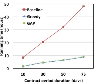
Fig. 6. Running time vs different contract period durations
0 10 20 30 40 50
99 99.9 99.99 99.999
Ru
nn
in
g
tim
e
(h
ou
rs
)
Availability requirement (%) Baseline
Greedy
GAP
Fig. 7. Running time vs different availability requirements
that particular path availability fromcandidate. The above procedure is repeated until a request is successfully mapped or considered rejected when there is no physical machine or bandwidth available.
V. EVALUATION
In this section, we evaluate the performance of our proposed algorithm in terms of 1) SFC request acceptance ratio, 2) backup resource consumed by requests and 3) running time. The distribution of device downtime is generated based on [19] and data collected from the Center for Computational Research (CCR), a large high performance computing facility at SUNY Buffalo [3, 15]. The statistics shown in this section are averaged outputs of the framework.
First we introduce two methods to see how our optimization performs.
1) Baseline: In the baseline method, backups are allocated followingAlgorithm 2.
2) Greedy: We modify the method in [17] to estimate the number of backups, where for an SFC request which requires n VNF and has the availability requirement of α, we keep increasing the number of backup for each VNF on all selected physical machines until each VNF can have an availability of √nα.
3) GAP: Backups are estimated following the optimization inAlgorithm 3.
Note that after estimating the number of backups needed using Greedy and GAP, more backups will be provisioned iteratively following the backup allocation method in Algo-rithm 2 until meeting the availability requirement. In all,
0 0.2 0.4 0.6 0.8 1
0 1 2 3 4
CD
F
[image:10.612.320.554.58.168.2]Number of iterations
Fig. 8. CDF of the number of iterations needed
Algorithm 2 is applied in all three methods to provision backups as it guarantees availability whileBaselinestarts with zero backup and the other two start with an estimated number of backups.
A. Running Time
One of the main benefits of an accurate estimation is to reduce the number of iterations that our framework needs to run, and therefore reduce the total running time. Note that the running time shown in this section includes both the estimation time used by our algorithms and the iterations to add more backups to guarantee availability. With the same example in Section III-D and K = 2, the total running time can be reduced to less than 5 hours, on 40 non-dedicated cores, which achieves a 87.5% improvement. Fig. 6 and Fig. 7 show the absolute running time with an SFC request which requires the same number of VNFs and VMs but different contract period durations and availability requirements, respectively. First, let’s compare the performance ofBaselineandGAP. It is clear that as the contract period duration increases, the running time of our framework increases almost proportionally, which is ex-pected as the number of samples is proportional to the duration of the contract period (See Section III-B). However, if our algorithm is first applied to estimate the number of backups, the growth rate is much smaller. Similar observations can be made when the availability requirement changes. Specifically, the running time with optimization keeps almost constant as the availability requirement increases (from 99% to 99.99%). When the availability is 99.99%, the relative improvement can be near 90%. The relative improvement is even higher when the availability requirement is further increased (i.e., 99.99%). The results imply that our optimization framework can help to estimate the number of backups needed, and we can save more time with higher availability requirements and longer contract period durations. Next, we compare the performance ofGreedy andGAP.Greedyrequires slightly less time than GAPas its estimation returns with a higher number of VMs (will be shown in the next section) and therefore a request is mapped with more backups.
We also evaluate our algorithm with SFC requests with different availability requirements, contract period durations, number of VNFs and number of VMs for each VNF. In total there are about 30 different cases with various combinations. The availability requirement of a request is selected among
[image:10.612.63.241.209.349.2]200 250 300 350 400
300 400 500
Numb
er of acce
p
ted r
equ
es
ts
Number of requests Baseline
[image:11.612.90.241.57.186.2]Greedy GAP
Fig. 9. Number of accepted requests with the Fat-tree topology
200 250 300 350 400 450
300 400 500
Numb
er of acce
p
ted r
equ
es
ts
Number of requests Baseline
[image:11.612.326.544.57.159.2]Greedy GAP
Fig. 10. Number of accepted requests with the BCube topology
of contract period duration is between 10 to 100 days. Fig. 8 shows the CDF of the number of extra iterations needed by our framework to provision availability after a request is mapped with GAP. For over three quarters of the time, only one iteration was required. As at least we need one iteration to verify if the returned result can achieve the availability requirement, this result shows that our optimization framework can return a solution within a single iteration with enough number of backups to guarantee availability in most cases. Multiple iterations are only needed in rare cases.
B. Resource Efficiency
Next, we run simulations to understand how the proposed algorithm can save resources. In our simulations, we use the 8-ary Fat-tree and the BCube(2, 5) topology so that they have a similar number of physical machines, and assume each physical machine can support up to 1024 VMs [2]. For each SFC request, the availability requirement is randomly selected among{99%, 99.9%, 99.99%, 99.999%, 99.9999%}, and the contract period duration is exponentially distributed with an average of 10 days. Each request consists of two to six VNFs, each of which demands a certain number of VMs that is uniformly distributed between 10 and 40 [17].
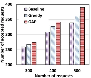
Fig. 9 and Fig. 10 shows the number of accepted requests with respect to different number of requests with two different topologies, respectively. In these simulations, the number of paths between the physical machines and all core switches K is set to 2 for both topologies. Clearly, with our backup selection method (i.e., GAP), the number of requests that can be accepted increases as the number of the requests increases.
10 12 14 16 18 20
99 99.9 99.99 99.999 99.9999
VM sa
ving p
er
ce
n
tag
es (%)
Availability requirements (%)
Fat-tree BCube
Fig. 11. Backup VM saving percentages
Furthermore, as the request number increases, we have a larger performance gain compared to Baseline and Greedy, since when the request number is small, VM resources are sufficient; while when there are more requests, the VM resources saved by GAP can be used to accommodate more requests. The reason is that with our algorithm, fewer backup VMs are required to reach a certain level of availability, as shown in Fig. 11, where the VM saving percentage is defined as
backup # w/ greedy - backup # w/ GAP
backup # w/ greedy given different availability re-quirements, and the request number is 400. Compared with Greedy, GAPcan save more resources while not increasing the running time. In addition, as depicted in these figures, more requests can be accepted with BCube compared to Fat-tree topology even though K is the same. This is because BCube is more robust to failures [21].
TABLE II
NUMBER OF ACCEPTED REQUESTS WITH DIFFERENTK
K 1 2 3 4
Number of accepted requests 285 327 328 302
To understand how K affects the performance, we run simulations in the same Fat-tree topology when there are 400 requests, and the number of accepted requests with different K value are shown in Table II. As mentioned, there is a trade-off between path availability of a physical machine and bandwidth consumption when adjustingK. From the table, we can see that when K is too small (i.e.,K = 1) or too large (i.e.,K = 4), the number of requests that can be accepted is smaller. Even thoughK= 3 gives up a slightly better result, the framework also needs to spend a longer time (about 30% more) to evaluate availability of a mapped request.
VI. RELATED WORK
Recently there are a number of works on network function placement with various objectives following the work of resource allocation in data centers [36, 39, 47, 52], such as energy efficiency and scalability. In [7], the authors not only consider the placement of VNFs but also derive the optimal resources needed to serve a given mobile traffic. Benkacem
[image:11.612.72.247.206.338.2]12
constraint. Cohenet. al.[12] studies a general NFV placement problem and provides an approximation algorithm. Laghrissi
et. al.[34] presents VNF placement algorithms to address the problem of non-uniform service demands and the irregular nature of network topologies by transforming physical domain signaling messages to canonical domain. Laghrissiet. al.[35] studies mobile service consumption behavior and presents a enhanced predictive VNF placement to consider both QoS and cost efficiency. Martini et. al. [38] studies the problem of composing and computing VNFs to select nodes along the path with the objective of minimizing end-to-end latency. Talebet. al.[50] optimizes VNF placement while considering operators’ cost as well as service usage behavioral patterns in a mobile environment.
However only few of them have considered the availabil-ity/reliability issues [17, 18, 43], let alone how to guarantee availability, which is considered as one of the most essen-tial topics in NFV [23]. Ding et. al. [14] proposes a new redundancy model by taking the global information of the VNF forwarding graph into consideration. In [16, 17], the authors proposed algorithms to provision availability with on-and off-site backups, but they assumed that only VMs would experience failures. In [25], the authors proposed resilient embedding algorithms in data centers for multiple backup strategies. In [29], the authors studied the tradeoff between reliability and computational due to replication of VNFs. Sun
et. al. [49] proposed algorithms to maximize the end-to-end availability while taking failures of both nodes and links into consideration. In [30], the authors proposed to optimize the backup scheme to maximize survivability while respecting the resource constraints. Qu et. al. [43] jointly optimizes VNF placement and traffic routing in data center networks to max-imize the reliability of network services and minmax-imize end-to-end service delay. Following this work, the authors further exploited the possibilities of backup resource sharing when provisioning SFC requests recently in [44]. However, none of these work considers the heterogeneous processes of devices’ failure and repair to the best of our knowledge. Kanizo et. al. [31] addressed the scheme for middlebox recovery with performance guarantees in a recent study, but the solution is applied to the case where only limited number of middleboxes can fail at the same time. In this paper, on the contrary, we propose a general framework to provision availability of NFV in data centers of arbitrary number of devices and improve the resource usage efficiency.
VII. DISCUSSION
Before concluding, we briefly discuss the usage issues of our framework in practice.
First, even though our optimization is able to reduce the total running time of the framework significantly, this procedure still requires a few hours to finish (Section V-A). Here, we list two potential solutions as we have seen that our optimization can achieve a reasonable estimation.
1) Based on our evaluations, sincefor requests with shorter contract time periods or less strict availability requirements, our algorithm can return enough backups, we can just use the
optimization to estimate backups needed for these requests; while for the rest requests, even though the estimated backups are not enough to provision availability, we know from Fig. 8 that we can achieve that by adding a few more backup VMs that would have been added during the iterations. There-fore, for requests with long contract time periods or strict availability requirementswe can map them with a few more backup VMs in addition to the estimated ones, as a possible upper limit on the VMs needed. Then we can accurately evaluate its availability using our framework after the request is deployed. If fewer backups are needed, we can retract the over-provisioned VMs.
2) We can further improve the estimation efficiency in III-B. Instead going over all possible states when estimating the downtime distribution, we can utilize importance sampling while having a very high accuracy.
Second, we made several assumptions that are simplifica-tions of reality when modeling the problem, which we intend to further explore as a future work. For example, we currently do not consider Byzantine failures of devices, which means devices, upon certain failures, can continue to work, but at a significantly reduced capacity. To incorporate this failure model, the definition of availability should also be modified that takes the processing rate of traffic into consideration. Besides, correlated failures such as failures due to power outages or configuration errors can have significant effects on service availability, which are not considered in this paper. One possible solution to address it is to identify/audit the independence of resources when allocating redundancy, and it requires a more detailed model of the system. Last but not least, for stateful VNFs, failovers from primaries to backups requires transferring of states, which makes the switching time not zero. We are currently working on a Generalized Stochastic Petri Net (GSPN) model to incorporate such an effect. More precisely, the switching from primaries to backups can be modeled as a timed transition, which means only after certain time (i.e., after the switching finishes), a backup can start and process traffic.
VIII. CONCLUSION
REFERENCES
[1] Amazon EC2 Pricing. https://aws.amazon.com/ec2/pricing.
[2] FusionSphere Cloud OS. http://e.huawei.com/us/products/cloud-computing-dc/cloud-computing/fusionsphere/fusionsphere.
[3] (2008). Reducing Data Center Cost with an Air Economizer. http://www.intel.com/it/pdf/Reducing Data Center Cost
with an Air Economizer.pdf.
[4] Al-Fares, M., Loukissas, A., and Vahdat, A. (2008). A scalable, com-modity data center network architecture. InACM SIGCOMM.
[5] Anderson, J. W., Braud, R., Kapoor, R., Porter, G., and Vahdat, A. (2012). xOMB: extensible open middleboxes with commodity servers. InACM/IEEE ANCS.
[6] Aven, T. and Jensen, U. (1999).Stochastic models in reliability. Springer. [7] Bagaa, M., Taleb, T., Laghrissi, A., Ksentini, A., and Flinck, H. (2018). Coalitional Game for the Creation of Efficient Virtual Core Network Slices in 5G Mobile Systems. IEEE Journal on Selected Areas in Communications, 36(3):469–484.
[8] Benkacem, I., Taleb, T., Bagaa, M., and Flinck, H. (2018). Optimal VNFs Placement in CDN Slicing Over Multi-Cloud Environment.IEEE Journal on Selected Areas in Communications, 36(3):616–627.
[9] Birolini, A. (2007). Reliability engineering, volume 5. Springer. [10] Bouet, M., Leguay, J., Combe, T., and Conan, V. (2015). Cost-based
placement of vDPI functions in NFV infrastructures.International Journal of Network Management, 25(6):490–506.
[11] Chakravarty, I. M., Roy, J., and Laha, R. G. (1967). Handbook of methods of applied statistics.
[12] Cohen, R., Lewin-Eytan, L., Naor, J. S., and Raz, D. (2015). Near optimal placement of virtual network functions. InIEEE INFOCOM. [13] Daskalakis, C., Diakonikolas, I., and Servedio, R. A. (2015). Learning
Poisson Binomial Distributions. Springer Algorithmica, 72(1):316–357. [14] Ding, W., Yu, H., and Luo, S. (2017). Enhancing the reliability of
services in NFV with the cost-efficient redundancy scheme. InIEEE ICC. [15] Du, A. Y., Das, S., Yang, Z., Qiao, C., and Ramesh, R. (2015). Predicting Transient Downtime in Virtual Server Systems: An Efficient Sample Path Randomization Approach.IEEE Transactions on Computers, 64(12):3541– 3554.
[16] Fan, J., Guan, C., Zhao, Y., and Qiao, C. (2017a). Availability-aware Mapping of Service Function Chains. InIEEE INFOCOM.
[17] Fan, J., Jiang, M., and Qiao, C. (2017b). Carrier-grade availability-aware mapping of Service Function Chains with on-site backups. InIEEE IWQoS.
[18] Fan, J., Ye, Z., Guan, C., Gao, X., Ren, K., and Qiao, C. (2015). GREP: Guaranteeing Reliability with Enhanced Protection in NFV. In ACM SIGCOMM Workshop on Hot Topics in Middleboxes and Network Function Virtualization.
[19] Gill, P., Jain, N., and Nagappan, N. (2011). Understanding network failures in data centers: measurement, analysis, and implications. InACM SIGCOMM.
[20] Greenhalgh, A., Huici, F., Hoerdt, M., Papadimitriou, P., Handley, M., and Mathy, L. (2009). Flow processing and the rise of commodity network hardware. ACM SIGCOMM CCR, 39(2):20–26.
[21] Guo, C., Lu, G., Li, D., Wu, H., Zhang, X., Shi, Y., Tian, C., Zhang, Y., and Lu, S. (2009). BCube: a high performance, server-centric network architecture for modular data centers. InACM SIGCOMM.
[22] Guo, C., Wu, H., Tan, K., Shi, L., Zhang, Y., and Lu, S. (2008). Dcell: a scalable and fault-tolerant network structure for data centers. InACM SIGCOMM.
[23] Han, B., Gopalakrishnan, V., Ji, L., and Lee, S. (2015). Network function virtualization: Challenges and opportunities for innovations.IEEE Communications Magazine, 53(2):90–97.
[24] Han, S., Jang, K., Panda, A., Palkar, S., Han, D., and Ratnasamy, S. Softnic: A software NIC to augment hardware. Dept. EECS, Univ. California, Berkeley, CA, USA, Tech. Rep. UCB/EECS-2015-155. [25] Herker, S., An, X., Kiess, W., Beker, S., and Kirstaedter, A. (2015).
Data-center architecture impacts on virtualized network functions service chain embedding with high availability requirements. InIEEE Globecom Workshops.
[26] Hong, Y. (2013). On computing the distribution function for the Poisson Binomial Distribution.Elsevier Computational Statistics & Data Analysis, 59:41–51.
[27] Hwang, J., Ramakrishnan, K. K., and Wood, T. (2015). NetVM: high performance and flexible networking using virtualization on commodity platforms. IEEE Transactions on Network and Service Management, 12(1):34–47.
[28] Jerrum, M. and Sinclair, A. (1996). The Markov chain Monte Carlo method: An approach to approximate counting and integration.
Approxi-mation algorithms for NP-hard problems, pages 482–520.
[29] Kang, J., Simeone, O., and Kang, J. (2017). On the trade-off between computational load and reliability for network function virtualization.IEEE Communications Letters, 21(8):1767–1770.
[30] Kanizo, Y., Rottenstreich, O., Segall, I., and Yallouz, J. (2017). Optimiz-ing virtual backup allocation for middleboxes.IEEE/ACM Transactions on Networking, 25(5):2759–2772.
[31] Kanizo, Y., Rottenstreich, O., Segall, I., and Yallouz, J. (2018). Design-ing Optimal Middlebox Recovery Schemes with Performance Guarantees. InIEEE INFOCOM.
[32] Kullback, S. and Leibler, R. A. (1951). On information and sufficiency. JSTOR The annals of mathematical statistics, 22(1):79–86.
[33] Kwisthout, J. (2011). Most probable explanations in Bayesian networks: Complexity and tractability.Elsevier International Journal of Approximate Reasoning, 52(9):1452–1469.
[34] Laghrissi, A., Taleb, T., and Bagaa, M. (2018). Conformal Mapping for Optimal Network Slice Planning Based on Canonical Domains. IEEE Journal on Selected Areas in Communications, 36(3):519–528.
[35] Laghrissi, A., Taleb, T., Bagaa, M., and Flinck, H. (2017). Towards edge slicing: VNF Placement algorithms for a dynamic & realistic edge cloud environment. InIEEE GLOBECOM, pages 1–6. IEEE.
[36] Li, X., Wu, J., Tang, S., and Lu, S. (2014). Let’s stay together: Towards traffic aware virtual machine placement in data centers. InIEEE INFOCOM.
[37] Mahadevan, P., Banerjee, S., Sharma, P., Shah, A., and Ranganathan, P. (2011). On energy efficiency for enterprise and data center networks. IEEE Communications Magazine, 49(8).
[38] Martini, B., Paganelli, F., Cappanera, P., Turchi, S., and Castoldi, P. (2015). Latency-aware composition of virtual functions in 5G. In IEEE NetSoft.
[39] Meng, X., Pappas, V., and Zhang, L. (2010). Improving the scalability of data center networks with traffic-aware virtual machine placement. In IEEE INFOCOM.
[40] Nemhauser, G. L., Wolsey, L. A., and Fisher, M. L. (1978). An analysis of approximations for maximizing submodular set functionsI. Springer Mathematical Programming, 14(1):265–294.
[41] Panda, A., Han, S., Jang, K., Walls, M., Ratnasamy, S., and Shenker, S. (2016). NetBricks: Taking the V out of NFV. InOSDI, pages 203–216. [42] Parzen, E. (1962). On estimation of a probability density function and
mode.JSTOR The annals of mathematical statistics, 33(3):1065–1076. [43] Qu, L., Assi, C., Shaban, K., and Khabbaz, M. (2017). A
Reliability-Aware Network Service Chain Provisioning with Delay Guarantees in NFV-Enabled Enterprise Datacenter Networks. IEEE Transactions on Network and Service Management.
[44] Qu, L., Khabbaz, M., and Assi, C. (2018). Reliability-aware service chaining in carrier-grade softwarized networks.IEEE Journal on Selected Areas in Communications, 36(3):558–573.
[45] Schlinker, B., Mysore, R. N., Smith, S., Mogul, J. C., Vahdat, A., Yu, M., Katz-Bassett, E., and Rubin, M. (2015). Condor: Better topologies through declarative design. InACM SIGCOMM.
[46] Sekar, V., Egi, N., Ratnasamy, S., Reiter, M. K., and Shi, G. (2012). Design and implementation of a consolidated middlebox architecture. In USENIX NSDI.
[47] Shrivastava, V., Zerfos, P., Lee, K.-W., Jamjoom, H., Liu, Y.-H., and Banerjee, S. (2011). Application-aware virtual machine migration in data centers. InIEEE INFOCOM.
[48] Sun, C., Bi, J., Zheng, Z., Yu, H., and Hu, H. (2017). NFP: Enabling Network Function Parallelism in NFV. InACM SIGCOMM.
[49] Sun, J., Zhu, G., Sun, G., Liao, D., Li, Y., Sangaiah, A. K., Ra-machandran, M., and Chang, V. (2018). A Reliability-Aware Approach for Resource Efficient Virtual Network Function Deployment. IEEE Access, 6:18238–18250.
[50] Taleb, T., Bagaa, M., and Ksentini, A. (2015). User mobility-aware virtual network function placement for virtual 5G network infrastructure. InIEEE ICC, pages 3879–3884. IEEE.
[51] Taylor, Z. and Ranganathan, S. (2013). Designing High Availability Systems: DFSS and Classical Reliability Techniques with Practical Real Life Examples. John Wiley & Sons.
[52] Wang, M., Meng, X., and Zhang, L. (2011). Consolidating virtual machines with dynamic bandwidth demand in data centers. In IEEE INFOCOM.
[53] Wang, Y. H. (1993). On the number of successes in independent trials. JSTOR Statistica Sinica, pages 295–312.
[54] Yeow, W.-L., Westphal, C., and Kozat, U. C. (2011). Designing and embedding reliable virtual infrastructures. ACM SIGCOMM CCR, 41(2):57–64.
water-14
filling for Gaussian vector multiple-access channels. IEEE Transactions on Information Theory, 50(1):145–152.
[56] Zhao, M. (1994). Availability for repairable components and series systems.IEEE Transactions on Reliability, 43(2):329–334.
Jingyuan Fanreceived the B.Eng. and M.S. degree from Fudan University, China, and the University of California, Los Angeles, USA, in 2012 and 2014, respectively. He is currently pursuing the Ph.D. de-gree with the Department of Computer Science and Engineering at University at Buffalo. His research interests lie in the field of computer networks.
Meiling Jiangreceived the MS degree in Applied Mathematics at State University of New York at Buffalo, New York, NY. She is currently working toward the PhD degree in the Department of Man-agement Science and Systems, State University of New York at Buffalo. Her research interest is in statistical modeling of availability in computing sys-tems, operations and economics of cloud computing markets, and healthcare analytics.
Ori Rottenstreichis with the faculty of Computer Science and the faculty of Electrical Engineering of the Technion, Haifa, Israel. His main research interest is computer networks. In 2015-2017 he was a Postdoctoral Research Fellow at the department of Computer Science, Princeton university. Earlier, he received the BSc in Computer Engineering (summa cum laude) and PhD degree from the Technion in 2008 and 2014, respectively.
Yangming Zhao is a research scientist at SUNY buffalo. He received the B.S. degree in communi-cation engineering and the Ph.D. degree in com-munication and information system from University of Electronic Science and Technology of China in 2008 and 2015, respectively. His research interests include network optimization, data center networks, edge computing and transportation systems.
Tong Guanreceived his B.S. degree in Electrical Engineering from Huazhong University of Science and Technology and received his Ph.D. Degree in Computer Science and Engineering from the Univer-sity at Buffalo in 2018. His research interests are in the areas of networking, mobile networks, and social networks with emphasis on mathematical modeling and performance analysis.
Ram Ramesh is Professor of Management Sci-ence & Systems, SUNY at Buffalo. His current research focuses on cloud infrastructure availabil-ity analytics. He serves as an Editor-in-Chief of Information Systems Frontiers and an Area Editor of INFORMS Journal on Computing for the area ”Knowledge Management and Machine Learning”. He has published extensively in ISR, INFORMS JoC, IEEE TKDE and many others. His research has been funded by NSF, AFOSR, ARL, ARI, Google, Raytheon, Samsung and Westinghouse among oth-ers.
Sanjukta Das an Associate Professor and Depart-ment Chair at SUNY Buffalo in the DepartDepart-ment of Management Science and Systems. She received her PhD in operations and information management in 2007 from the University of Connecticut. Her research interests include resource allocation and contract design in cloud computing. Her research has been funded by Google and NSF. She has published extensively in journals such as INFORMS Journal on Computing and Information Systems Research. She serves as an Associate Editor for Information Systems Research. She has served as an Associate Editor for INFORMS Journal on Computing, as a Coordinating Editor for Information Systems Frontiers, and as a Guest Associate Editor for MIS Quarterly.
![Fig. 2. Case study: a 4-ary Fat-tree data center topology [4]](https://thumb-us.123doks.com/thumbv2/123dok_us/8350520.309522/2.612.151.460.57.184/fig-case-study-fat-tree-data-center-topology.webp)