S O F T W A R E
Open Access
Python algorithms in particle tracking
microrheology
Timo Maier
1,2and Tam´as Haraszti
1,2*Abstract
Background: Particle tracking passive microrheology relates recorded trajectories of microbeads, embedded in soft samples, to the local mechanical properties of the sample. The method requires intensive numerical data processing and tools allowing control of the calculation errors.
Results: We report the development of a software package collecting functions and scripts written in Python for automated and manual data processing, to extract viscoelastic information about the sample using recorded particle trajectories. The resulting program package analyzes the fundamental diffusion characteristics of particle trajectories and calculates the frequency dependent complex shear modulus using methods published in the literature. In order to increase conversion accuracy, segmentwise, double step, range-adaptive fitting and dynamic sampling algorithms are introduced to interpolate the data in a splinelike manner.
Conclusions: The presented set of algorithms allows for flexible data processing for particle tracking microrheology. The package presents improved algorithms for mean square displacement estimation, controlling effects of frame loss during recording, and a novel numerical conversion method using segmentwise interpolation, decreasing the conversion error from about 100% to the order of 1%.
Keywords: Particle tracking microrheology, Numerical conversion method, Software library, Dynamic interpolation
Background
Particle tracking microrheology is a modern tool to inves-tigate the viscoelastic properties of soft matter, for exam-ple, biopolymers and the interior, or the membrane of living cells [1,2] on the microscopic scale. Though embed-ding tracer particles into such a sample alters the local structure, this method is still considered non-invasive and provides important information not available by other methods [1-4].
The physical background of the method lies in the ther-mal motion of the tracer particle, which can be connected to the viscoelastic properties of the local environment through the generalized Langevin equation [5,6]. Neglect-ing the inertia term, which contributes to frequencies in the megahertz range, and assuming that the memory function is linearly related to the frequency dependent
*Correspondence: [email protected]
1Max-Planck Institute for Intelligent Systems, Advanced Materials and Biosystems, Heisenberg str. 3, 70569 Stuttgart, Germany
2Biophysical Chemistry, Institute of Physical Chemistry, University of Heidelberg, Im Neuenheimer Feld 253, 69120 Heidelberg, Germany
viscosity of the medium (through a generalized Stokes-Einstein relation)[3,5-8], the mean square displacement (MSD) of the particle can be directly related to the creep compliance as:
J(τ )= 3πa NDkBT
< r2(τ ) >, (1)
whereτ denotes the time step in which the particle moves
rdistance,< r2(τ ) >the mean square displacement, NDthe dimensionality of the motion (usuallyND = 2 for particle tracking digital microscopy),kB the Boltzmann constant,Tis the absolute temperature andathe particle radius, respectively.
Active microrheology (using optical or magnetic tweez-ers) and macroscopic rheometry commonly characterize the sample elasticity with the frequency-dependent com-plex shear modulus,G∗(ω), which is a complex quantity [4,9,10]. Its real part is known as the storage modulus
G(ω)and the imaginary part is the loss modulus,G(ω). WhileJ(t)is a description in the time domain,G∗(ω)is an equivalent characterization in the frequency domain.
The two types of description are equivalent and intercon-nected with the relation:
G∗(ω)= 1
iωJ˜(ω), (2)
where˜J(ω)is the Fourier transform ofJ(t). Assuming that the particle tracks are previously obtained, the frequency dependent complex shear modulusG∗(ω)can be derived using equations (1) and (2) after calculating the mean square displacement.
There are two major algorithm libraries available on the Interned addressing data handling for microrheology: the algorithm collection of J. Crocker et al. written in the interactive data language (IDL) [11], which was translated to Matlab and expanded by the Kilfoil lab [12]. A sepa-rate stand alone algorithm is provided by M. Tassieri for calculating the complex shear modulus from the creep compliance, written in LabView [13]. However, an exten-sible integrated framework relying on freely accesexten-sible software and source code integrating multiple conversion methods is not yet available.
In this paper we present a software package written in the interpreted programing language Python (http://www. python.org) collecting functions to support particle track-ing microrheology related calculations, with emphasis on those parts providing enhanced functionality. This library is meant to be an open source, platform independent, freely extendable set of algorithms allowing to extract rheology information from particle tracks obtained previously.
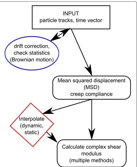
The Rheology software library contains two example scripts. One called ProcessRheology.py, a configuration driven program performing all processing steps from par-ticle trajectory inputs, thus presenting the various capa-bilities of the library (Figure 1). This program can be employed as a self-standing calculator or its code can be used as a template for the user testing the Rheology library. The other is theFunction-test.py, containing test calculations, and which was also employed to produce the figures in this article (see the content of the Additional file 1).
Implementation Dependencies
The software depends on the following Python packages for calculations and displaying results:
• Numpy:a library for array manipulation and calculations [14];
• Scipy:the Python scientific library, from which we used the gamma function and the nonlinear least squares fitting function [14];
• Matplotlib:a Matlab-like plotting library to generate information graphs of the results [15].
Figure 1Process flow chart of microrheology data.The fundamental processing steps in particle tracking microrheology as followed by theProcessRheology.pyscript. There are several parameters that may affect the details of the process, including the sampling in the MSD calculation and which way the complex shear modulus is calculated (see the main text for details). In this article we focus mainly on the later tree steps in the process: the MSD calculation and conversion methods.
After installation, its functions are available using fol-lowing import command within the interpreter or a Python script:
from Rheology import *
Data presentation, data format
Instead of defining individual classes for each data type (MSD, creep compliance and complex shear modulus), an alternative technique in Python is to employ generalized lists, the so called dictionaries or ‘dicts’. A dict is a con-tainer class holding data which are indexed with arbitrary keys (marked by quotes in this paper). This is a very gen-eral and flexible data structure, which we used for all data in the Rheology package. For example, MSD dicts contain keys “tau” and “MSD” referring to arrays holding the time lag and the mean square displacement data, respectively.
Particle trajectories
sense, however, obtaining particle trajectories from video microscopy is well described in the literature [16-20] including the statistical difficulties of the process [21-23]. There are various implementations of particle tracking algorithms available in IDL (see the same website as for the rheology code) [11,24], Matlab [12,25], LabView [20,26] or C++ languages [27]. An implementation of the Grier method [16] is also translated to Python [28].
Thus, we start our discussion by extracting rheologi-cal information from the particle trajectories, leaving the implementation of data input/output to the user. As a good starting template, we recommend theReadTable()
andSaveTable()functions in theProcessRheology.py exam-ple script.
Drift correction
Several experimental systems show a drift: a slow oriented motion of the sample versus the imaging frame, which is caused by various factors of the experimenting apparatus. To remove this drift, which is independent of the sam-ple, there are multiple possibilities one may consider. If a reference bead bound to the sample is available, its tra-jectory provides the drift itself. If multiple particles are tracked in the same time interval, an average trajectory may be calculated and used as a reference. If these pos-sibilities are not available, one has to consider whether the long time motion is due to drift or it is a charac-teristic of the investigated sample, because subtracting it changes the resulted long time lag (low frequency) part of the viscoelastic characteristics.
The simplest way of data treatment in such cases is to calculate a smoothened trajectory: e. g. using a run-ning average, and either subtract this smoothened data or, in one further step, fit a low order polynomial to the smoothened data and subtract the fitted values from the trajectory.
A very simple implementation is available for two dimensional data sets as:
GetData(timestamps, poslist, indx=0, order=3,resolution=0.1434, Nd= 1000)
This algorithm takes a position list (parameterposlist), which is a list of dicts, each describing the positions of a particle. Theindxparameter is used to select one of them. A position dict contains “X”, and “Y”, which are arrays of the x and y positions. The dict also contains an index array denoted with key “indx”, identifying the image index (serial number) of the given positions. Using this index allows the tracking algorithm to miss individual frames (e. g. when the particle drifted out of focus). This index is also used to define the time point of a position, either by identi-fying the corresponding time stamps, provided in seconds in thetimestampsarray, or if this variable is set to None,
multiplying the index by the optional tscale parameter. TheNdparameter gives the number of points used in the running average and the order parameter identifies the order of the polynomial to be fitted for drift correction. If
Ndis set to−1, the running averaging is off, and iforderis -1, the drift correction is turned off. Theresolutionis used to scale the coordinates to micrometers (the same value for both coordinates).
Mean square displacement (MSD)
Characterizing a soft sample using particle tracking microrheology strongly relies on the determination of the mean square displacement. Calculating the MSD has two possible sets of assumptions: 1.) ensemble averages are based on recording many tracer particles and assum-ing homogeneity across the sample. This is the averagassum-ing method considered in theories, and has the advantage allowing estimation of the time-dependent aging of the system. Technically this can be achieved by using video recording-based particle tracking, where the number of tracers can be increased to the order of tens. 2.) Assum-ing ergodicity, one can switch from ensemble averagAssum-ing to time averaging. This is very important for systems which are not homogeneous and for cases where only few par-ticles (1−5) can be observed at a time. For samples of biological origin, time averaging is more suitable because these samples are seldom homogeneous.
Calculating the time average is done by splitting up the trajectory into non-overlapping parts and averaging their displacement. Because the number of intervals decreases with an increasing lag time, this method has very high error for large lag time values. Alternatively, it is also pos-sible to split the trajectory into overlapping regions and then do the averaging. The resulting statistical errors fol-low a non-normal distribution, but it has been shown that using overlapping segments the resulted MSD may show improved accuracy [29,30] when using lag time values up to about the quarter of the measurement length (N/4 for
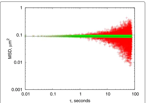
Ndata points). The results of a test calculation using posi-tions randomly calculated from a normal distribution with standard deviation ofσX = σY = 0.15μmin both X and Y directions are presented in Figure 2. The MSD oscil-lates around the theoretical value of< r(τ )2>=2(σX2+ σY2)=0.09μm2as expected, but the data calculated using overlapping intervals show visibly better accuracy.
msd = MSD(positionlist, tau= 0)
MSD()is the function to calculate the mean square dis-placement from a single trajectory. The data points are presented as a two dimensional arraypositionlist, contain-ing coordinates ((x,y)or(x,y,z)) in each row.
0.001 0.01 0.1 1
0.01 0.1 1 10 100
MSD,
μ
m
2
τ, seconds
Figure 2mean square displacement data calculated from simulated data.The distribution of X and Y positions were generated based on a normal distribution withσ =0.15μm. The theoretical MSD is constant at 0.09μm2(black line). Data with non-overlapping intervals (red+symbols) show higher scattering, the ones calculated with overlapping intervals (green×) show a much lower error.
parameter can take various values: If an array or list of integer values are given, then those are used as index step values. If a single integer is given between 0 and the num-ber of positions, then so many index steps (lag time values) are generated in an equidistant manner. If nothing, or 0 is given, then values 1. . .N/4 are used.
Each tau value results in M = M(tau) pairs, where the stepr[i+tau]−r[i] is calculated.Malso depends on whether the set was generated using overlapping intervals (ifoverlap=Trueis set).
If an array of time values (in seconds) are provided for the position data using the optionaltvectorparameter, the algorithm will check the time step between each data pair used. Calculating the mean value of these time steps and using a relative error, every value outside themean(1±
tolerance) will be ignored (by defaulttolerance = 0.1). This process eliminates jumps in the data caused by com-puter latency during recording.
The function returns a dictionary containing “tau”, “dtau”, “MSD”, “DMSD” keys. If the time values were not provided, then “tau” holds the index steps between the positions and “dtau” is not used.
Creep compliance
Assuming that the generalized Stokes-Einstein relation holds, the creep compliance is linearly proportional to the MSD [6]. The MSD to J()function calculates the creep compliance using equation (1).
J = MSD to J(msd, t0= 0.1, tend= 150, T= 25.0, a= 1.0)
The calculation requires a dict structure (msd) having the time values under the “tau” key, and the MSD values
under the “MSD” key (error values are optional). Further parameters are the temperature T of the experiment in Celsius degrees, the radiusaof the applied tracer particle in micrometers, and optionally the dimensionality of the motionD(denoted asNDin equation (1)), which is set to D=2 by default.
Calculating the frequency dependent shear modulus fromJ(t)with the numerical method proposed by Evans et al. requires extrapolated values to the zero time point and to infinite time values. These values are estimated here, allowing the user to override them before being used to calculate the complex shear modulusG∗(ω). The zero time valueJ0 = J(t = 0)is extrapolated from a linear fit in thet<t0 region, and the end extrapolation is obtained from a linear fit to the tend < tpart. The slope of the extrapolated end part is 1/η, whereηis the steady state viscosity [31].
The function returns a new dict containing: “J” (in 1/Pa), “tau”, “eta”, “J0”, “const”, “dJ”, and the fit parameters as “a0”, “b0” for the first part and “a1”, “b1” for the end part, where the linear equationJ=ait+bi(i=0, 1)holds.
Calculating the frequency dependent complex shear modulus
While the connection presented by equation (2) is simple, there is a major problem with determining˜J(ω) numeri-cally. It is well known in numerical analysis that applying a numerical Fourier transform increases the experimen-tal noise enormously [32]. In microrheology, there are four commonly applied methods to solve this problem. The first two address the noise of the Fourier transform directly by averaging or by fitting, the second two were suggested in the last decade to improve the transform itself [6,9,31-33].
In a homogeneous system, where multiple particles can be tracked, converting their MSD to creep compliance and thenG∗(ω)using a discrete Fourier transform, allows one to average the converted values and decrease the noise this way [32,33]. For cases when the creep compliance can be modeled using an analytical form, the Fourier trans-form of the fitted analytical function may be calculated and used to estimate ofG∗(ω)[9].
Because these methods have their strength and weak-ness, we summarize them and their implementation below. Recently we have shown that the accuracy of the Evans method can be greatly improved by using local interpolation of the data in a splinelike manner without forcing a single function to be fitted to the whole data set. This improvement is also included in the Rheology framework and will be discussed below.
The Mason method
This is a fast conversion method based on the Fourier transformation of a power function, which has been used in various works in the last decade [6-8,37-39]. Briefly, let us consider a generalized diffusion process, where the MSD is following a power law:< r(t)2 >= 2NDDtα [40], whereDis the generalized diffusion coefficient, and 0 < α ≤2. In the case ofα = 1 we can talk about regu-lar Brownian diffusion,α <1 describes subdiffusion and
α > 1 superdiffusion, indicating active forces participat-ing in the process. Usparticipat-ing the generalized Stokes-Einstein equation (1) we consider Brownian and subdiffusion pro-cesses, thusα≤1 [5,40]. In this case the creep compliance will also be described with a power function as:
J(t)=J0tα (3)
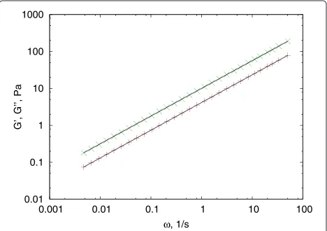
The complex shear modulus can be directly calculated using a gamma function (Figure 3), in the form of:
G∗(ω)=eiπ α2 ω
α
J0 (1+α) =
eiπ α2
J(t=1/ω) (1+α). (4)
Usually this equation is presented containing the MSD [41], but the key feature, the symmetry between the time dependent creep-compliance and the frequency
0.01 0.1 1 10 100 1000
0.001 0.01 0.1 1 10 100
G’, G’’, Pa
ω, 1/s
Figure 3Testing the Mason method.Complex shear modulus (storage modulus (red+) and loss modulus (green×)) calculated from a power law creep compliance in the form ofJ(τ )=0.1τ0.75
and converted using theJ to G Mason()function and theoretically (solid line) using equation (4).
dependent complex shear modulus, is more apparent in this form. The method generalizes this symmetry between
ω ↔ t : ω = 1/t, and assumes it holds for the whole measured time range [6], even when the exponentαof the power law varies with time.
However, this is a highly specific case, and the symmetry does not hold for most of the functions [41]. To improve the fit quality, a slightly more complicated version of this formula has been proposed by Dasgupta et al. in [38], based on empirical corrections.
The J to G Mason()function implements both meth-ods based on references [6,38] and theleastsq()function of scipy, which is a modified Levenberg-Marquardt mini-mization algorithm.
G = J to G Mason(J,N=30, advanced=True, logstep=True)
The algorithm takes a creep-compliance dict (J), and fits a power function locally in the form of equation (3) to estimate α and calculates the complex shear modu-lus atω = 1/t using equation (4). The algorithm uses a Gaussian function to weight the neighbors in the local fit as it is described by Mason et al. [6]. N defines the desired number of resulted data points, which are created by equidistant sampling in the linear or logarithmic space between 1/tmax. . .1/tmin. The logarithmic sampling is activated by thelogstepparameter, which is set by default. The resulted dict contains ’omega’ and ’f ’ for the circu-lar frequency and frequency respectively, and a ’G’ array storing the corresponding complex shear moduli.
There are several further parameters to control the pro-cess, from which setting theadvanced parameter forces the use of the method proposed by Dasgupta et al. instead of the original Mason method, and theverboseswitch pro-vides graphical feedback on how the local fitting proceeds. A test example is presented in Figure 3 using a creep compliance in the form of equation (3) and converted both numerically and analytically. Because this method is accurate for power law creep compliances, the conversion matches within machine precision.
The Evans method
The fourth method we again discuss in detail. It is based on the work published by Evans et al. [31]. This method considers a linear interpolation between theNdata points and provides a conversion in the form of equation (5)[41].
G∗(ω)= iω
iωJ0+Nk=0(Ak+1−Ak)e−iωtk
, (5)
whereAis are defined by:
Ak=
Jk−Jk−1 tk−tk−1
, where0<k≤N,A0=0,AN+1= 1
η.
J0 and η are already estimated using the linear fits in the MSD to J()function. Using equation (5) is straight-forward, and allow for the calculation ofG∗(ω)at anyω
values. The natural selection of a suitable frequency range would be from 0 toNπT (the unit is 1/s) inN/2 steps as it is common for the discrete Fourier transform of equally sampled data [32]. The corresponding function is:
G = J to G(J)
The algorithm generates a linear array of frequencies, but the number of points is limited to be maximum 1000, usually more than sufficient (MSD and creep compliance data arrays may hold several thousand points). The result is a similar dictionary as it was for the Mason method, and can be tested using a Maxwell-fluid, which has a lin-ear creep compliance in the form of J(t) = 1/E+ t/η
(Figure 4).
There are various details worth mentioning about this method, which may affect the accuracy of the result in general cases. It is clear in equation (5), that the method is sensitive to theAk+1−Akterms, which, in extreme cases, may be either very small for a nearly linear part ofJ(t)or very high for sudden jumps in the experimental data. In order to reduce round-off errors, one may eliminate the close to zero values, (when|Ak+1−Ak|< ε) by activating thefilterparameter.
This numerical conversion method has two basic prob-lems. First, from equation (5) it is apparent that the complex shear modulus is directly related to the numeri-cal Fourier transform of theAk+1−Akset, and thus very sensitive to the noise of these data. Second, the limited
0.0001 0.001 0.01 0.1 1 10
0.1 1 10 100 1000
G’, G’’, Pa
ω, 1/s
Figure 4Maxwell fluid, testing the Evans method.The complex shear modulus of a Maxwell fluid with Young modulus ofE=10Pa and viscosityη=0.2Pas, calculated usingJ to G()(symbols) and analytically (solid line). The storage modulus (red+) and loss modulus (green×) data calculated numerically fits well to the theoretical values presented by the solid black lines.
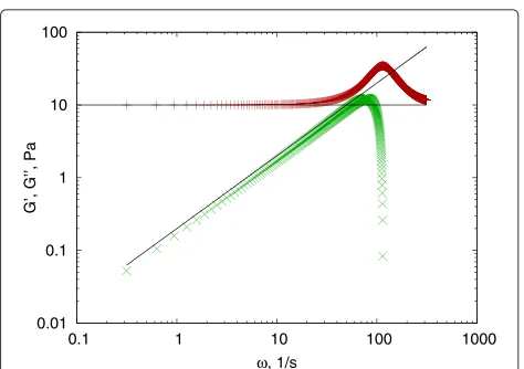
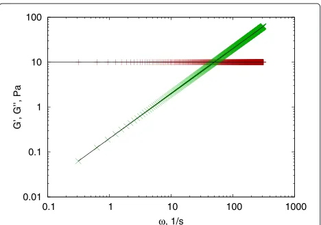
bandwidth causes the Ak values to be a poor represen-tation of the local derivative of the creep compliance, resulting in a strong deviation (usually an unphysical cut-off ) of the calculated shear modulus. This latter problem is well represented on a test example of a Kelvin-Voigt solid characterized by a Young’s modulus of E = 10Paand viscosityη=0.2Pas(Figure 5).
The conversion can be improved by increasing the bandwidth of the data, or decreasing the frequency range whereG∗(ω)is calculated (using theomaxparameter). A third alternative is using model interpolations to increase the bandwidth numerically. Because most experimental data cannot be fitted with a single analytical function for allτvalues, we have developed a method to fit the MSD at consecutive intervals in a splinelike manner [41].
Adaptive splinelike fitting
Biopolymer samples commonly show monotonic MSD, frequently described by power laws at various time seg-ments. This makes the choice of the power function a good candidate for the local fitting. To count for devi-ations from power laws at short time values, the fitting system also allows the use of a Kelvin-Voigt solid as an alternative model for short time scales, in the case of more elastic samples. Including a Maxwell fluid as an option was not necessary, since the Evans method provides perfect fits for linear MSDs (see Figure 4).
Because this algorithm has not been published pre-viously, we describe it here in detail. The procedure is designed to run automatically being controlled only by selecting the start interval of the data and a scaler, which defines how fast the fitting range should increase with time. The key steps are:
0.01 0.1 1 10 100
0.1 1 10 100 1000
G’, G’’, Pa
ω, 1/s
1. define the data range using indicesi0=0and i1=i(t0), containing at least 4 data points;
2. fit function fromi0. . .i1, calculate the squared error of each point and estimate the average error; 3. find the last point aroundi1whereχ2(i2) < χmean2
and redefinei1as this pointi1=i2(stretching or shrinking the fitting range to a reasonable maximum) 4. recalculate the fit and errors, store as the current
segment
5. if we reached the end (or close to the end), finish the cycle, return with the results
6. otherwise, define the new fitting range, using the scaler parameter (by default usei0. . .scaler×i0) 7. return to 2 (see Additional file 1)
The exact procedure calculating the new range in each step may vary depending on themode an optional key-word parameter, allowing for some control for functions which show fast changes or slow changes with noise. The default method (mode=“scaler”) described above works well for most MSDs with some noise but monotonic trends. (More details are available in the help of the library and theconfig.exampletext file in the Examples folder of the package).
The corresponding function call is:
fits = MSD power fit(msd, t0=0.2, scaler=10.0).
Completing the above algorithm, in the next step the program checks where the fits would cross each-other in the neighboring ranges, and readjusts them to the crossing point, if it lies within the union of the two ranges. This step helps to maintain a smoother approximation of the exper-imental data. Turning verbosity on using verbose=True, one may see details about how the algorithm operates.
Dynamic and static interpolation
The return value (fits) is a list of dicts, each containing the fitting parameters of one segment. This list can be directly used to calculate the interpolation of the original data using:
msd2 = MSD interpolate(msd, fits, smoothing = True, Nsmoothing=10, insert=10,
factor=3)
The interpolation and insertion of new points before the first data point will increase the bandwidth of the origi-nal data. Thefactorparameter controls the oversampling of the original data (here it is set to 3× oversampling). Inserting new data points between 0 and the first timeτ0 is specified byinsert=10.
Estimating how many new points are required during this resampling procedure is a difficult question in general.
The above example uses a static approach, simply insert-ingfactorpoints between every two original data points, which results in a very large equidistant data set. Alterna-tively we provide a dynamic method, which is controlled by an error parameter.
Investigating the form of equations (2) and (6), one can see that the accuracy of the Evans method is strongly related to how accurately equation (6) approximates the local derivative of J(t). Knowing the analytical form of the interpolating functions, this error can be approxi-mated using the function (f) and its second derivative (f”) [32,41]. Based on this approximation and specifying a local errorε, the minimal step size at any time pointh(t)
can be estimated as:
h=ε
fk(tk) fk(tk)
. (7)
Using h as a minimal step size for each fitted seg-ment, the program can dynamically interpolate the data and increase the number of points only where the creep compliance changes faster. This results in a non-equally sampled data set, which (after calculating the creep com-pliance) can be well handled by both theMSD to J() func-tion and subsequently the numerical conversion method
J to G(), resulting in an improved complex shear modu-lus. To eliminate further bandwidth problems, the maxi-mal desired circular frequencyωmaxcan be forced to NTπ using theomaxparameter.
The consequence of this fitting and interpolation pro-cedure is an increased bandwidth and decreased noise in the interpolated data set. The resulting accuracy is some orders of magnitude larger than the specifiedεbut strongly related to it. Therefore the user has to estimate the suitableεfor the given problem. For example, insert-ing 10 new points between 0 − t0 and requesting an accuracy ofε = 5×10⁻⁴, the algorithm has corrected the errors of Figure 5 to about 1% relative error on aver-age (Figure 6). The Mason method produces about 100% relative error for the loss modulus of the same conversion, originating from the failure of its power law assumption, and can not be improved by interpolation [41].
0.01 0.1 1 10 100
0.1 1 10 100 1000
G’, G’’, Pa
ω, 1/s
Figure 6Dynamic resampling.Dynamic resampling can correct the errors of the Evans method resulting in an improved fit. The storage modulus (red+) and loss modulus (green×) data calculated numerically shows a good fit to the theoretically predicted values (black lines).
defined by theNSmoothparameter. The range is identi-fied in the original data, but then applied to the refined data set. The result is an MSD, where sudden jumps are reduced, minimizing the presence of oscillatory artifacts in the resulted complex shear modulusG∗(ω).
Conclusions
In this paper we have presented a free software solution for analyzing particle tracking data for microrheology. Our software library implements the time average calcu-lation of mean square displacement with control over the time shift in the data, and conversion methods to calcu-late the creep compliance and the complex shear modulus. Beyond the two most common methods mentioned in the literature, we have developed a dynamic local fitting pro-cedure, which allows spline-like fitting of the MSD and improved conversion accuracy to about 1% from about 100% for a Kelvin-Voigt model test.
Availability and requirements
Lists the following:
• Project name:Rheology for Python • Project home page:http://launchpad.net/
microrheologypy/
• Operating systems:Platform independent (Linux, Windows and Max OSX tested)
• Programing language:Python 2.7
• Other requirements:Numpy 1.5, Scipy 0.1, Matplotlib 1.0
• License:LGPL v3
• Any restrictions to use by non-academics:see license
Additional file
Additional file 1: rheology.zip - compressed ZIP archive containing the Rheology Python package.The archive contains several files. The source code in the Rheology subfolder, a setup.py for installation, README.txt and License.txt files and the Example subfolder. Installation (as usual in python):
python setup.py build; python setup.py install
The Example subfolder contains two Python scripts. The Function-test.py can be used to run test calculations and see the example plots presenting that all functions work properly. The figures presented in this paper were also generated by this script.
The ProcessRheology.py is a batch processing script, controlled by commands and parameters provided in a config.txt plain text file. An example of this file is also included here, containing detailed description of every parameter. This scripts is a fully functioning microrheology data evaluation toolkit, utilizing the functions of the Rheology package.
Abbreviations
MSD, Mean square displacement.
Competing interests
The Authors declare that they have not competing interests.
Authors’ contributions
TM and TH have developed the Python software together discussing and testing the various features, and both contributed to writing this manuscript. Both authors read and approved the final manuscript.
Acknowledgements
This work was supported by the Ministry of Science, Research, and the Arts of Baden-W ¨urttemberg (AZ:720.830-5-10a). The authors would like to thank to Professor Dr. Joachim P. Spatz, Dr. Heike Boehm and the Max-Planck Society for the generous financial support and Dr. Claire Cobley for assistance.
Received: 13 September 2012 Accepted: 14 November 2012 Published: 27 November 2012
References
1. Dangaria JHH, Butler PJJ:Macrorheology and adaptive microrheology of endothelial cells subjected to fluid shear stress.Am J Physiol Cell Physiol2007,293:C1568—C1575.
2. Bausch AR, Moller W, Sackmann E:Measurement of local viscoelasticity and forces in living cells by magnetic tweezers.Biophys J1999, 76:573–579.
3. Waigh TA:Microrheology of complex fluids.Rep Prog Phys2005, 68(3):685.
4. Wirtz D:Particle-tracking microrheology of living cells: principles and applications.Annu Rev Biophys2009,38:301–326.
5. Mason TG, Weitz DA:Optical measurements of frequency-dependent linear viscoelastic moduli of complex fluids.Phys Rev Lett1995, 74(7):1250–1253.
6. Mason TG, Ganesan K, van Zanten JH, Wirtz D, Kuo SC:Particle tracking microrheology of complex fluids.Phys Rev Lett1997,79:3282 – 3285. 7. Mason TG:Estimating the viscoelastic moduli of complex fluids using
the generalized Stokes-E, instein equation.Rheologica Acta2000, 39(4):371–378.
8. Squires TM, Mason TG:Fluid mechanics of microrheology.Annu Rev Fluid Mech2010,42:413–438.
9. Goodwin JW, Hughes RW:Rheology for Chemists. An Introduction. Second edition. Cambridge: RSC Publishing; 2008.
10. Mezger TG:The Rheology Handbook. 3rd revised edition. Vincentz Network GmbH & Co. KG , Plathnerstr. 4c, Vol. 30175. Hannover, Germany: European Coatings Tech Files, Vincentz Network; 2011.
12. Kilfoil M, et al.:Matlab algorithms from the Kilfoil lab.[http://people. umass.edu/kilfoil/downloads.html]
13. Tassieri M:Compliance to complex moduli, version 2.2011. [https:// sites.google.com/site/manliotassieri/labview-codes]
14. Jones E, Oliphant T, Peterson P, et al.:SciPy: Open source scientific tools for Python.2001. [http://www.scipy.org/]
15. Hunter JD:Matplotlib: A 2D graphics environment.Comput Sci Eng
2007,9(3):90–95. [http://matplotlib.sourceforge.net/]
16. Crocker JC, Grier DG:Methods of digital video microscopy for colloidal studies.J Colloid Interface Sci1996,179:298–310. [http://www. physics.emory.edu/weeks/idl/]
17. Brangwynne CP, Koenderink GH, Barry E, Dogic Z, MacKintosh FC, Weitz DA:Bending dynamics of fluctuating biopolymers probed by automated high-resolution filament tracking.Biophys J2007, 93:346–359.
18. Gosse C, Croquette V:Magnetic tweezers: micromanipulation and force measurement at the molecular level.Biophys J2002, 82(6):3314–3329.
19. Rogers SS, Waigh TA, Lu JR:Intracellular microrheology of motile amoeba proteus.Biophys J2008,94(8):3313–3322.
20. Carter BC, Shubeita GT, Gross SP:Tracking single particles: a user-friendly quantitative evaluation.Phys Biol2005,2:60.
21. Savin T, Doyle PS:Statistical and sampling issues when using multiple particle tracking.Phys Rev E2007,76(2):021501.
22. Savin T, Doyle PS:Static and dynamic errors in particle tracking microrheology.Biophys J2005,88:623–638.
23. Savin T, Spicer PT, Doyle PS:A rational approach to noise
discrimination in video microscopy particle tracking.App Phys Lett
2008,93(2):024102.
24. Smith R, Spaulding G:User-friendly, freeware image segmentation and particle tracking.[http://titan.iwu.edu/gspaldin/rytrack.html] 25. Blair D, Dufresne E:The Matlab particle tracking code
respository.:2005 - 2008. [http://physics.georgetown.edu/matlab/] 26. Milne G:Particle tracking.2006. [http://zone.ni.com/devzone/cda/epd/
p/id/948]
27. Caswell TA:Particle identification and tracking.[http://jfi.uchicago. edu/tcaswell/track doc/]
28. Haraszti T:ImageP: image processing add-ons to Python and numpy. 2012 2009. [https://launchpad.net/imagep]
29. Flyvbjerg H, Petersen HG:Error estimates on averages of correlated data.J Chem Phys1989,91:461–466.
30. Saxton M:Single-particle tracking: the distribution of diffusion coefficients.Biophys J1997,72(4):1744–1753.
31. Evans RML, Tassieri M, Auhl D, Waigh TA:Direct conversion of rheological compliance measurements into storage and loss moduli.Phys Rev E2009,80:012501.
32. Press WH, Teukolsky SA, Vetterling WT, FB P:Numerical recipes in C++. second edition. Cambridge: Cambridge University Press; 2002. 33. Addas KM, Schmidt CF, Tang JX:Microrheology of solutions of
semiflexible biopolymer filaments using laser tweezers interferometry.Phys Rev E2004,70(2):021503.
34. Morse DC:Viscoelasticity of concentrated isotropic solutions of semiflexible polymers. 2. Linear Response.Macromolecules1998, 31(20):7044–7067.
35. Morse DC:Viscoelasticity of concentrated isotropic solutions of semiflexible polymers. 1. model and stress tensor.Macromolecules
1998,31(20):7030–3043.
36. Gittes F, Schnurr B, Olmsted PD, MacKintosh FC, Schmidt CF:Microscopic viscoelasticity: shear moduli of soft materials determined from thermal fluctuations.Phys Rev Lett1997,79(17):3286–3289. 37. Crocker JC, Valentine MT, Weeks ER, Gisler T, Kaplan PD, Yodh AG, Weitz
DA:Two-point microrheology of inhomogeneous soft materials.
Phys Rev Lett2000,85(4):888–891.
38. Dasgupta BR, Tee SY, Crocker JC, Frisken BJ, Weitz DA:Microrheology of polyethylene oxide using diffusing wave spectroscopy and single scattering.Phys Rev E2002,65(5):051505.
39. Cheong F, Duarte S, Lee SH, Grier D:Holographic microrheology of polysaccharides from streptococcus mutans biofilms.Rheologica Acta
2009,48:109–115.
40. Tejedor V, Benichou O, Voituriez R, Jungmann R, Simmel F,
Selhuber-Unkel C, Oddershede LB, Metzler R:Quantitative analysis of single particle trajectories: mean maximal excursion method.
Biophys J2010,98(7):1364–1372.
41. Maier T, Boehm H, Haraszti T:Splinelike interpolation in particle tracking microrheology.Phys Rev E2012,86:011501.
doi:10.1186/1752-153X-6-144
Cite this article as:Maier and Haraszti:Python algorithms in particle track-ing microrheology.Chemistry Central Journal20126:144.
Open access provides opportunities to our colleagues in other parts of the globe, by allowing
anyone to view the content free of charge.
Publish with
Chemistry
Central and every
scientist can read your work free of charge
W. Jeffery Hurst, The Hershey Company.
available free of charge to the entire scientific community peer reviewed and published immediately upon acceptance cited in PubMed and archived on PubMed Central yours you keep the copyright
Submit your manuscript here: