Global stability analysis of an SVEIR epidemic model with general incidence rate

R E S E A R C H

Open Access

Global stability analysis of an SVEIR

epidemic model with general incidence rate

Da-peng Gao

_{, Nan-jing Huang}

_{, Shin Min Kang}

_{and Cong Zhang}

*_{Correspondence:} [email protected]; [email protected] 2_{Department of Mathematics,} Sichuan University, Chengdu, P.R. China

4_{School of Management, Sichuan} University of Science and Engineering, Zigong, P.R. China Full list of author information is available at the end of the article

Abstract

In this paper, a susceptible-vaccinated-exposed-infectious-recovered (SVEIR)

epidemic model for an infectious disease that spreads in the host population through horizontal transmission is investigated, assuming that the horizontal transmission is governed by an unspecified functionf(S,I). The role that temporary immunity (vaccinated-induced) and treatment of infected people play in the spread of disease, is incorporated in the model. The basic reproduction numberR0is found, under

certain conditions on the incidence rate and treatment function. It is shown that the model exhibits two equilibria, namely, the disease-free equilibrium and the endemic equilibrium. By constructing a suitable Lyapunov function, it is observed that the global asymptotic stability of the disease-free equilibrium depends onR0as well as

on the treatment rate. IfR0> 1, then the endemic equilibrium is globally

asymptotically stable with the help of the Li and Muldowney geometric approach applied to four dimensional systems. Numerical simulations are also presented to illustrate our main results.

MSC: 92D25; 92D30; 34D23; 37B25

Keywords: Epidemic model; Reproduction number; Lyapunov function; Geometric approach; Global stability; Susceptible–Vaccinated–Exposed–Infectious–Recovered

1 Introduction

Mathematical modeling enjoys popularity in both preventing and controlling infectious diseases such as severe acute respiratory syndrome (SARS) [1], human immunodeficiency virus infection/acquired immune deficiency syndrome (HIV/AIDS) [2], H5N1 (avian flu) [3] and H1N1 (swine flu)[4]. In recent years, a lot of efforts have been made to develop realistic diseases and further study the asymptotic behavior of such epidemic models [5]. In the field of studying epidemic model behavior, one of the most important parts is to analyze steady states together with their stability [6]. In general, there are two distinct techniques named Lyapunov’s direct method and Li–Muldowney’s geometric approach to give sufficient conditions of global stability for the equilibrium states (see, for exam-ple, [7–14]). We would like to mention some related work concerned with the existence of positive solutions for the discrete fractional boundary value problem [15], the sensitiv-ity analysis for optimal control problems governed by nonlinear evolution inclusions [16] and the nonexistence of global in time solution of the mixed problem for the nonlinear evolution equation with memory generalizing the Voigt–Kelvin rheological model [17].

It is well known that the rate of incidence plays the main part in modeling infectious diseases. The rise and fall of epidemics can be influenced by some factors, such as density of population and life style [18, 19]. Many researchers have adopted different nonlinear incidence rates in their works. For more details, we refer the reader to [8–14, 20–34] and the references therein. When it comes to control of a disease, it is generally known that the spread of many diseases can be prevented by vaccinating. When massive vaccination is impossible, the second stage of defensive mechanism could be medical treatment. Individ-uals need to bear in mind that the treatment is an indispensable way to take precautions for some diseases (for instance, measles, phthisis and influenza). In recent years, many treat-ment functions have been introduced by several authors to study some epidemic models under different conditions (see, for instance, [12, 14, 27, 31, 35–38]).

Recently, Dénes and Röst [27] investigated the followingSImodel:

⎧ ⎪ ⎪ ⎨ ⎪ ⎪ ⎩

dS

dt =μ–f(S,I) –μS, dI

dt=f(S,I) –g(I),

1 =S+I+R,

(1.1)

where a population of constant size (assumed to be equal to 1) is divided into three com-partments: susceptible (denoted byS), infected (denoted byI) and recovered (denoted byR). The transmission of the infection is governed by the incidence ratef(S,I) andμis birth rate as well as the death rate of the susceptible class. The nonlinear functiong(I) de-notes the sum of the death rate and the recovery rate for the infected individuals satisfying g(0) = 0 andg(I) > 0 forI> 0. Using a Dulac function approach, which aims at eliminating the existence of the periodic solution and proving the global stability by the Poincaré-Bendixson theorem (see [39], p. 54), they obtained the global stability of the disease-free equilibrium and the endemic equilibrium for system (1.1).

Very recently, Upadhyay et al.[12] considered the following e-epidemic model:

⎧ ⎪ ⎪ ⎪ ⎪ ⎪ ⎪ ⎪ ⎪ ⎨ ⎪ ⎪ ⎪ ⎪ ⎪ ⎪ ⎪ ⎪ ⎩

dS

dt =A–δ0S–

αSI

S+I+c+ηV–μS, dE

dt =

αSI

S+I+c– (δ0+δ1)E, dI

dt=δ1E– (δ0+δ2+δ3)I–

βI I+a, dR

dt =δ2I–δ0R+

βI I+a, dV

dt =μS– (δ0+η)V.

(1.2)

Using a Lyapunov function and a geometric approach, they obtained the global stability of virus-free equilibrium and endemic equilibrium for system (1.2).

As pointed out by Liu and Yang [11], due to the high similarity between computer virus and biological virus, it is acceptable to establish dynamical models describing biological virus among a population by modifying an e-epidemic model. Thus, it is interesting and important to extend model (1.2) to study the biological virus in the infectious disease.

Inspired by these research results above, in this paper, we consider the following system with five compartments:

⎧ ⎪ ⎪ ⎪ ⎪ ⎪ ⎪ ⎪ ⎪ ⎨ ⎪ ⎪ ⎪ ⎪ ⎪ ⎪ ⎪ ⎪ ⎩

dS

dt =A–δ0S–f(S,I) +ηV–μS, dE

dt =f(S,I) – (δ0+δ1)E, dI

dt=δ1E– (δ0+δ2+δ3)I–g(I), dR

dt =δ2I–δ0R+g(I), dV

dt =μS– (δ0+η)V,

(1.3)

whereS(t),E(t),I(t),R(t),V(t) are the number of susceptible population, exposed popula-tion, infective populapopula-tion, recovered populapopula-tion, vaccinated populapopula-tion, respectively. The two-variable functionf(S,I) represents incidence rate and the nonlinear functiong(I) de-notes the removal rate of infective individuals because of the treatment of infective. The initial conditions for system (1.3) are as follows:

S(0) =S0≥0, E(0) =E0≥0, I(0) =I0≥0,

R(0) =R0≥0, V(0) =V0≥0.

(1.4)

Clearly,N=S(t) +E(t) +I(t) +R(t) +V(t) denotes the total number of high-risk human population at timet.

The model parameters of system (1.3) are described as follows:

A: the rate at which new individuals (including newborns and immigrants) enter the susceptible population,

δ0: natural death rate of population all classes,

η: the rate at which the vaccinated population lose their immunity and join the suscep-tible class,

μ: vaccination rate coefficient,

δ1: the rate at which exposed population become infective,

δ2: natural recovery rate of infective population,

δ3: disease-related death rate of infective population.

Model (1.3) involves certain assumptions which consist of the following:

(i) The new individuals enter the population with a constant rate and all the new individuals are susceptible.

(ii) Susceptible individuals move to exposed class by adequate contact with infective individuals and after some time (i.e., latency period), they become infectious and move to infectious class.

(iii) The infectious individuals are assumed to leave the infectious class as a result of natural death and disease-related death as well as recovery of infected individuals. (iv) After recovery the individuals become immunized and hence they are no longer

(v) It is assumed that a fraction of susceptible individuals get vaccinated and join the vaccinated class. A part of vaccinated individuals may lose their immunity and rejoin the susceptible class.

It is easy to see that system (1.3) includes (1.1) and (1.2) as special cases and so model (1.3) provides a uniform setting for the computer virus and biological virus studies. Fol-lowing the classical assumptions [27, 40], it is reasonable to suppose that the transmission of the infection is governed by an incidence ratef(S,I) in model (1.3). Moreover, as pointed out by Wang [31], the recovery rate is naturally dependent on the number of infected in-dividuals provided the health care resources are constrained and so it is natural to use the nonlinear functiong(I) as the treatment function in model (1.3).

The main purpose of this paper is to derive the expression for the basic reproduction number and further show the global stability of disease-free as well as endemic equilibria by the aid of Lyapunov function and Li–Muldowney geometric approach applied to four dimensional systems. This paper is organized as follows. In Sect. 2, some elementary as-sumptions on the functionsf andgwill be given, and the basic reproduction numberR0 is provided. Also the equilibrium points are discussed. The global stability of disease-free equilibrium and endemic equilibrium are analyzed in Sects. 3 and 4, respectively. All our important analytical findings are numerically verified with the help of Mathlab in Sect. 5. Finally, a brief conclusion is given in Sect. 6.

2 Basic reproduction number and equilibrium

To define the basic reproduction numberR0and indicate the existence of equilibrium, we give some hypotheses.

(H1) f :R2₊→R+is differentiable such that f(S, 0) =f(0,I) = 0for allS,I≥0;

f(S,I) > 0for allS,I> 0;

∂f(S,I)

∂S > 0for allS≥0andI> 0;

∂f(S,I)

∂I ≥0for allS,I≥0;

I∂f_∂(S_I,I)–f(S,I)≤0for allS,I≥0.

(H2) g:R+→R+is differentiable such thatg(0) = 0,g(I) > 0andg(I)≤0forI≥0. (H3) _dId(logg(I)

fS(I))≥0holds for allS,I> 0, wherefS(I) :=f(S,I)forS,I> 0.

Remark2.1

(1) It is easy to check that the classes off(S,I)satisfying (H1) include incidence rates such as

f(S,I) = βSI

1 +aIq, f(S,I) = βSI

1 +aS+bI, f(S,I) =

βSI 1 +aS+bI+abSI,

forβ,a,b> 0and0≤q≤1.

(2) It is straightforward to show that the classes ofg(I)satisfying (H2) include removal rates such as

g(I) = rI

1 +bI, g(I) = rI

I+a, g(I) =rarctanI,

(3) By hypothesis (H2), we know thatΦ(I) =g(_II) is a monotone decreasing function on I> 0.

(4) The assumption (H3) is equivalent to the following inequality:

∂

∂If(S,I)g(I)≤f(S,I) d dIg(I),

which can be found in [27].

(5) By the assumptions, it is easy to find that system (1.3) always has a disease-free equilibrium pointP0= (S0, 0, 0, 0,V0), where

S0=

(δ0+η)A

δ2

0+ (μ+η)δ0

, V0=

Aμ δ2

0+ (μ+η)δ0 .

We shall assume that (H1), (H2) and (H3) hold in the rest of this paper. Now we define the basic reproduction numberR0for model (1.3) as follows:

R0=

δ1 m2(m3+g(0))

∂f

∂I

A m1–_mμη₄

, 0

,

where

m1=δ0+μ, m2=δ0+δ1, m3=δ0+δ2+δ3, m4=δ0+η.

In order to find the positive equilibria of model (1.3), set

⎧ ⎪ ⎪ ⎪ ⎪ ⎪ ⎨ ⎪ ⎪ ⎪ ⎪ ⎪ ⎩

A–f(S,I) –m1S+ηV= 0,

f(S,I) –m2E= 0,

δ1E–m3I–g(I) = 0,

δ2I–δ0R+g(I) = 0, μS–m4V= 0.

(2.1)

It follows thatA–m1S+ηV=m2E=m2m3I+g(I)

δ1 andV=

μS m4.

Substituting the above equalities into the second equation in (2.1), one has

f

_A–m2m3I+m2g(I)

δ1

m1–_mμη

4

,I

=m2

m3I+g(I)

δ1 .

Let

F(I) =f

_A–m2m3I+m2g(I)

δ1

m1–_mμη₄ ,I

–m2m3I+g(I)

δ1

. (2.2)

Then it is easy to see that the positive equilibrium points of system (2.1) are given by zeros ofFin the interval (0, Aδ1

m3m2].

We denoteG(I) =m3I+g(I) –Aδ1

m2 for convenience. Then it is easy to see

G(0) = –Aδ1

m2 < 0, G

Aδ1 m3m2

=g

Aδ1 m3m2

Therefore, we conclude thatG(I) has at least one root namedI˜in the interval (0, Aδ1 m3m2].

That is,m3˜I+g(˜I) = A_mδ₂1 and so

F(˜I) =f

_A–m2m3I˜+m2g(˜I)

δ1

m1–_mμη

4

,I˜

–m2m3I˜+g(˜I)

δ1

= –m2

Aδ1 m2 δ1

= –A< 0.

Sincef(S, 0) = 0, we know that_∂∂f_S(_m A

1–mμη4

, 0) = 0 and so

F(0) =∂f

∂I

A m1–_mμη

4 , 0 –m2 δ1

m3+g(0) =m2

δ1

m3+g(0)(R0– 1).

IfR0> 1, then system (2.1) has a positive equilibrium pointP∗= (S∗,E∗,I∗,R∗,V∗), where

S∗=A–

m2m3I∗+m2g(I∗)

δ1

m1–_mμη

4

, E∗=m3I ∗_+g(I∗₎

δ1 ,

R∗=δ2I ∗_+g(I∗₎

δ0

, V∗=μS ∗

m4 .

In the following, we show thatP∗ is the unique positive equilibrium point of system (2.1). For any positive equilibrium pointP∗, by (2.2) and hypotheses (H1) and (H2), we have

FI∗ =∂f(S ∗_,I∗₎

∂S

(–m2)(m3+g(I∗))

δ1(m1–_mμη₄)

+∂f(S ∗_,I∗₎

∂I

–m2(m3+g _(I∗₎₎

δ1

. (2.3)

Sincem1m4= (δ0+μ)(δ0+η) >μηand hypotheses (H1) and (H2) hold, we have

∂f(S∗,I∗)

∂S

1 m1–μη_m4

–1

δ1

m2m3+m2gI∗ < 0. (2.4)

Sinceg(0) = 0 andgis differentiable onR+, there existsξ∈(0,I∗) such that g(I ∗₎

I∗ =g(ξ).

By using hypotheses (H2) and (H3), one has

∂f(S∗,I∗)

∂I –

m2

δ1

m3+g

I∗ =∂f(S ∗_,I∗₎

∂I –

f(S∗,I∗) m3I∗+g(I∗)

m3+g

I∗

< f(S

∗_,I∗_)g(I∗₎

g(I∗) –

f(S∗,I∗)(m3+g(I∗)) m3I∗+g(I∗)

=fS∗,I∗ g _(I∗₎

g(I∗) –

m3+g(I∗) m3I∗+g(I∗)

=fS∗,I∗ m3I

∗_g(I∗_{) –m} 3g(I∗) g(I∗)[m3I∗+g(I∗)]

=fS∗,I∗ m3I

∗_[g(I∗_{) –}g(I∗)

I∗ ]

=fS∗,I∗ m3I

∗_[g(I∗_{) –g(ξ)]}

g(I∗)[m3I∗+g(I∗)]

< 0. (2.5)

Thus, it follows from (2.3), (2.4) and (2.5) thatF(I∗) < 0.

Suppose that there exists another positive equilibrium pointP1= (S1,E1,I1,R1,V1). Then F(I1)≥0 due to the property of continuous function. This is a contradiction. Therefore, system (2.1) has a unique endemic equilibriumP∗whenR0> 1. It can be stated as follows.

Theorem 2.1 System(1.3)has a disease-free equilibrium P0as follows:

P0=

(δ0+η)A

δ₀2+ (μ+η)δ0

, 0, 0, 0, Aμ

δ₀2+ (μ+η)δ0

,

which exists for all parameter values.ForR0> 1,the endemic equilibrium P∗admits the unique positive equilibrium point for system(1.3).

Remark2.2 From the proof of the existence of endemic equilibriumP∗, it is not difficult to arrive at such a conclusion that the nonlinear treatment functiong(I) has an upper bound

Aδ1

m2, which is reasonable for limited medical resources in our daily life.

Proposition 2.1 The set

Ω=

(S,E,I,R,V)∈R5₊, 0 <S,E,I,R,V,S+E+I+R+V≤ A

δ0

is a positively invariant and attracting region for the disease transmission model given by system(1.3)with initial conditions(1.4).

Proof Summing up the five equations in system (1.3) and denoting

N(t) =S(t) +E(t) +I(t) +R(t) +V(t),

we get

dN(t)

dt =A–δ0N–δ3I≤A–δ0N,

i.e.,

dN(t)

dt +δ0N≤A.

Now integrating both sides of the above inequality and using the theory of differential inequality [41], we obtain

0 <N≤

N(0)e–δ0t₊A δ0

1 –e–δ0t _.

Clearly, 0 <N≤ _δA

0 ast→ ∞. IfN(0)≤ A

δ0, thenN(t)≤ A

δ0. Thus, the setΩ is

3 Global stability of the disease-free equilibrium by means of Lyapunov function

In this section, we investigate the global stability of the disease-free equilibriumP0 for system (1.3).

Theorem 3.1 IfR0< 1 –

Ag(0)–δ0g(δA₀)

A(m3+g(0)) ,then the disease-free equilibrium P0of system(1.3) is globally asymptotically stable in the feasible regionΩ.IfR0> 1,then P0is unstable.

Proof The Jacobian matrix of system (1.3) atP0is

J(P0) =

⎛ ⎜ ⎜ ⎜ ⎜ ⎜ ⎜ ⎜ ⎝

–m1 0 –∂_∂f_I( (δ0+η)A

δ₀2+(μ+η)δ0, 0) 0 η

0 –m2 ∂_∂f_I( (δ0+η)A

δ2₀+(μ+η)δ0, 0) 0 0

0 δ1 –m3–g(0) 0 0 0 0 δ2+g(0) –δ0 0

μ 0 0 0 –m4

⎞ ⎟ ⎟ ⎟ ⎟ ⎟ ⎟ ⎟ ⎠ .

Obviously,λ1= –δ0is an eigenvalue ofJ(P0). The other eigenvalues ofJ(P0) are determined by the equations

λ2+ (m1+m4)λ+ (m1m4–μ) = 0

and

λ2+m2+m3+g(0) λ+m2m3+g(0) (1 –R0) = 0,

respectively. IfR0> 1, then one eigenvalue is positive. Thus,P0is unstable.

WhenR0< 1 –

Ag(0)–δ0g(_δA

0)

A(m3+g(0)) , to prove the disease-free equilibriumP0is globally

asymp-totically stable, we consider the Lyapunov functionV(E,I) =δ1E+m2I. The derivative of V(E,I) along system (1.3) satisfies

dV(E,I) dt =δ1

f(S,I) –m2E +m2

δ1E–m3I–g(I)

=δ1f(S,I) –m2m3I+g(I)

=I

δ1

f(S,I) I –m2

m3I+g(I) I

≤I

δ1

f(_m A

1–μηm4

,I)

I –m2

m3+ g(I)

I

≤I

δ1 lim

I→0+

f(_m A

1–mμη4

,I)

I –m2

m3+g(I) I

=I

δ1

∂f( A m1–mμη₄, 0)

∂I –m2

m3+g(I) I =I m2

m3+g(0) R0–m2

m3+ g(I)

I

=Im2m3+g(0) R0–

m2(m3+g(_II)) m2(m3+g(0))

=Im2m3+g(0) R0– 1 +

m3+g(0) –m3–g(_II) m3+g(0)

≤Im2

m3+g(0) R0– 1 +

Ag(0) –δ0g(_δA

0)

A(m3+g(0))

≤0.

Furthermore, dV_dt(E,I) = 0 iffI= 0. Thus, the largest compact invariant set in{(S,E,I,R,V)| ˙

V(E,I) = 0}, whenR0< 1 –

Ag(0)–δ0g(_δA 0)

A(m3+g(0)) , is the singletonP0. By the LaSalle invariance

prin-ciple theorem ([42], p. 30), the disease-free equilibriumP0is globally asymptotically stable

ifR0< 1 –

Ag(0)–δ0g(δA0)

A(m3+g(0)) . This completes the proof.

4 Global stability of the endemic equilibrium by means of geometric approach In this section, we analyze the stability of the endemic equilibriumP∗. First, we show the local stability of the endemic equilibrium of system (1.3) around the endemic equi-libriumP∗.

Theorem 4.1 IfR0> 1,then the endemic equilibrium P∗exists and is locally asymptoti-cally stable if the following conditions hold:

(i) η<a11m4

μ ;

(ii) a13<min{a11m4+(a11+m4)(a33+m2)+a33m2–μη δ1 ,

a11(a33+m2)m4+a33(a11+m4)m2–μη(a33+m2)

(m1+m4)δ1 , a11a33m2m4–μηa33m2

(m1m4–μη)δ1 };

(iii) 0 <h≤_a z

33m4+(a33+m4)m2 and

a11>(a33μm2η–a21a13m4δ1)h2–a13δ1h(μηh+z)+a33hz(m2+m4)+hz(m2m4–μη)–z2 h[a33m2m4h–a13m4δ1h–(a33+m2+m4)z] .

Here all the parametersa11,a13,a21,a33,a43are defined in(4.1).The values ofh

andzequal toB1andB3,respectively.

Proof The Jacobian matrix of system (1.3) atP∗is given by

JP∗ =

⎛ ⎜ ⎜ ⎜ ⎜ ⎜ ⎜ ⎝

–a11 0 –a13 0 η

a21 –m2 a13 0 0

0 δ1 –a33 0 0 0 0 a43 –δ0 0

μ 0 0 0 –m4

⎞ ⎟ ⎟ ⎟ ⎟ ⎟ ⎟ ⎠

,

where

a11=∂f(S ∗_,I∗₎

∂S +m1, a13=

∂f(S∗,I∗)

∂I ,

a21=∂f(S ∗_,I∗₎

∂S , a33=m3+g

_I∗ _{, a43=δ} 2+g

I∗ .

(4.1)

Clearly, one of the roots ofJ(P∗) is negative, i.e. –δ0. The remaining roots can be deter-mined from the following equation:

where

B1=a11+a33+m2+m4> 0,

B2=a11m4+ (a11+m4)(a33+m2) +a33m2–μη–δ1a13,

B3=a11(a33+m2)m4+a33(a11+m4)m2–μη(a33+m2) –δ1a13(m1+m4),

B4=a11a33m2m4–a33μηm2–δ1a13m1m4+δ1a13μη.

Using assumptions (i) and (ii), by a direct calculation, we haveBi> 0 fori= 1, 2, 3, 4. It

follows from the Routh–Hurwitz criteria [43] that all the eigenvalues associated toJ(P∗) have negative real parts iffBi> 0 fori= 1, 2, 3, 4 andB1B2B3>B23+B21B4.

Now,

B1B2B3–B2₃–B2₁B4

=B3(B1B2–B3) –B2₁B4

=a11(a33+m2)m4+a33(a11+m4)m2–μη(a33+m2) –δ1a13(m1+m4)

·a11(a11+m4)m4+ (a11+m4)2_{(a33+m2) + (a11+m4)(a33+m2)}2

+a33(a33+m2)m2– (a11+m4)μη–δ1a13(a21+a33+m2)–B4h2

= –B4h2+ha11m4+ (a11+m4)(a33+m2) +a33m2–μη–δ1a13z

–a11(a33+m2)m4+m2a33(a11+m4) –μη(a33+m2)

–δ1a13(m1+m4)z

= –B4h2+ha33m4+ (a33+m4)m2+a11(a33+m2+m4) –μη–δ1a13z

–a11a33m4+a33m2m4+a11(a33+m4)m2– (a33+m2)μη

–δ1a13(m1+m4)z

= –B4h2+ha33m4+ (a33+m4)m2+a11(a33+m2+m4) –μη–δ1a13z

–a11a33m4+a33m2m4+a11(a33+m4)m2– (a33+m2)μη

–δ1a13(m1+m4)2

> 0,

if (iii) holds. This ends the proof.

To find the global stability of system (1.3), it is necessary to reduce system (1.3) first. Since recovered classRdoes not have any effect on the dynamics ofS,V,EandIclass, we shall investigate the following system:

⎧ ⎪ ⎪ ⎪ ⎪ ⎪ ⎨ ⎪ ⎪ ⎪ ⎪ ⎪ ⎩

dS

dt =A–δ0S–f(S,I) +ηV–μS, dE

dt =f(S,I) – (δ0+δ1)E, dI

dt=δ1E– (δ0+δ2+δ3)I–g(I), dV

dt =μS– (δ0+η)V.

The solutions of (4.2) corresponding to nonnegative initial values remain nonnegative for all time. Moreover, we observe that the total population size of (4.2) denoted byX(t) satisfiesX˙ =A–δ0X–δ2I–δ3I–g(I), so that we can study the model in the region:

Θ=

(S,E,I,V)∈R4₊:S+E+I+V≤ A

δ0

.

Here we follow the approach used in [8] for a SVEIR model of SARS epidemic spread. Let us consider the following autonomous dynamical system:

˙

x=f(x), (4.3)

wheref:D→Rn,D⊂Rnwhich is an open set, simply connected andf ∈C1_{(D). Suppose} thatx∗ is an equilibrium point of (4.3), i.e.f(x∗) = 0. Therefore,x∗ is said to be globally stable inDif it is locally stable and all trajectories inDconverge tox∗.

LetQ(x) be a matrix-valued function of ordern₂ ×₂n that isC1onD. We also consider the matrixAwhich is defined as

A=QfQ–1+QMQ–1,

where the matrixQf is

qij(x)_f =

∂qij(x) ∂x

T

·f(x) =∇qij·f(x),

and the matrixMis the second additive compound matrix of the Jacobian matrixJ. Further

the Lozinski˘i measureμ¯ ofAwith respect to a vector norm · can be defined in R

_n

2 _as follows:

¯

μ(A) = lim

h→0+

I+hA

h .

We will apply the following theorem according to [44].

Lemma 4.1 If D1is a compact absorbing subset in the interior of D,and there existγ > 0 and a Lozinski˘i measureμ¯(A)≤–γ for all x∈D1,then every omega limit point of system (4.2)in the interior of D is an equilibrium in D1.

Theorem 2.1 states thatR0> 1 implies the existence and uniqueness of the endemic equilibriumP∗. Further, we know that the disease-free equilibriumP0 is unstable when

R0> 1. The instability ofP0, together withP0∈∂Θ, which implies the uniform persistence of the state variables (see [45]). Thus, there exists a constanta> 0 such that any solution (S(t),E(t),I(t),V(t)) with (S(0),E(0),I(0),V(0)) in the orbit of system (4.2) satisfies

min

lim

t→∞infS(t),tlim→∞infE(t),tlim→∞infI(t),tlim→∞infV(t)

≥a.

According to [47], the Lozinski˘i measure in Lemma 4.1 can be evaluated as:

¯

μ(A) =infk¯:D+z ≤ ¯kz, for all solutions of z=Az,

where D+ is the right-hand derivative. The endemic equilibrium is locally asymptoti-cally stable, provided R0> 1. Hence, to get the global asymptotic stability, according to Lemma 4.1, the trick of the proof is to find a norm · such thatμ¯(A) < 0 for allxin the interior ofΘ.

Starting with the Jacobian matrixJof (4.2),

J=

⎛ ⎜ ⎜ ⎜ ⎝

a11 a12 a13 a14 a21 a22 a23 a24 a31 a32 a33 a34 a41 a42 a43 a44

⎞ ⎟ ⎟ ⎟ ⎠,

the second additive compound matrix is given by

⎛ ⎜ ⎜ ⎜ ⎜ ⎜ ⎜ ⎜ ⎜ ⎝

a11+a22 a23 a24 –a13 –a14 0

a32 a11+a33 a34 a12 0 –a14

a42 a43 a11+a44 0 a12 a13

–a31 a21 0 a22+a33 a34 –a24

–a41 0 a21 a43 a22+a44 a23

0 –a41 a31 –a42 a32 a33+a44

⎞ ⎟ ⎟ ⎟ ⎟ ⎟ ⎟ ⎟ ⎟ ⎠

.

Hence, the second additive compound matrix ofJis given as follows:

M=

⎛ ⎜ ⎜ ⎜ ⎜ ⎜ ⎜ ⎜ ⎜ ⎝

M11 M12 0 M14 M15 0

M21 M22 0 0 0 M26

0 0 M33 0 0 M36

0 M42 0 M44 0 0

M51 0 M53 0 M55 M56

0 M62 0 0 M65 M66

⎞ ⎟ ⎟ ⎟ ⎟ ⎟ ⎟ ⎟ ⎟ ⎠

,

where

M11= –2δ0–

∂f(S,I)

∂S – (μ+δ1), M12=

∂f(S,I)

∂I ,

M14=∂f(S,I)

∂I , M15= –η;

M21=δ1, M22= –2δ0–

∂f(S,I)

∂S –μ– (δ2+δ3) –g

_{(I), M} 26= –η;

M33= –2δ0–

∂f(S,I)

∂S – (μ+η), M36= –

∂f(S,I)

∂I ;

M42=∂f(S,I)

∂S , M44= –2δ0– (δ1+δ2+δ3) –g _(I);

M51= –μ, M53=∂f(S,I)

M56=∂f(S,I)

∂I , M62= –μ, M65=δ1;

M66= –2δ0– (δ2+δ3+η) –g(I).

Now we consider the following matrix:

Q= ⎛ ⎜ ⎜ ⎜ ⎜ ⎜ ⎜ ⎜ ⎜ ⎝ 1

I 0 0 0 0 0

0 1

I 0 0 0 0

0 0 0 1_I 0 0 0 0 _V1 0 0 0 0 0 0 0 _V1 0

0 0 0 0 0 1

V ⎞ ⎟ ⎟ ⎟ ⎟ ⎟ ⎟ ⎟ ⎟ ⎠ . (4.4)

Then we obtain the matrixA=QfQ–1+QMQ–1, whereQf is the derivative ofQin the

direction of the vector fieldf. More accurately, we have

QfQ–1= –diag _˙ I I, ˙ I I, ˙ I I, ˙ V V, ˙ V V, ˙ V V .

Hence, in view of the fact that

˙ I I =δ1

E

I – (δ0+δ2+δ3) – g(I)

I , ˙ V V =μ

S

V – (δ0+η),

we obtain A= ⎛ ⎜ ⎜ ⎜ ⎜ ⎜ ⎜ ⎜ ⎜ ⎝

A11 A12 A13 0 A15 0

A21 A22 0 0 0 A26

0 A32 A33 0 0 0

0 0 0 A44 0 A46

A51 0 0 A54 A55 A56

0 A62 0 0 A65 A66

⎞ ⎟ ⎟ ⎟ ⎟ ⎟ ⎟ ⎟ ⎟ ⎠ , where

A11=g(I)

I +δ2+δ3–δ0–δ1–δ1 E I –

∂f(S,I)

∂S –μ,

A12=

∂f(S,I)

∂I , A13=

∂f(S,I)

∂I , A15= –η V

I;

A21=δ1, A22= –δ0–

∂f(S,I)

∂S –μ–g

_{(I) +}g(I) I –δ1

E

I, A26= –η V

I;

A32=∂f(S,I)

∂S , A33=

g(I)

I – (δ0+δ1) –g _{(I) –δ}

1 E

I;

A44= –δ0–

∂f(S,I)

∂S –μ–μ S

V, A46= –

∂f(S,I)

∂I ;

A51= –μI

V, A54=

∂f(S,I)

∂S , A55= –μ S

V – (δ0+δ1), A56=

∂f(S,I)

∂I ;

A62= –μI

V, A65=δ1, A66= –(δ0+δ2+δ3) –g

As in [8], we consider the following norm onR6_:

z=max{U1,U2}, (4.5)

where z∈R6, with componentszi,i= 1, 2, . . . , 6, andU1(z1,z2,z3) is defined as:

U1(z1,z2,z3)

=

⎧ ⎪ ⎪ ⎪ ⎪ ⎪ ⎨ ⎪ ⎪ ⎪ ⎪ ⎪ ⎩

max{|z1|,|z2|+|z3|}, if sgn(z1) =sgn(z2) =sgn(z3),

max{|z2|,|z1|+|z3|}, if sgn(z1) =sgn(z2) = –sgn(z3),

max{|z1|,|z2|,|z3|}, if sgn(z1) = –sgn(z2) =sgn(z3),

max{|z1|+|z3|,|z2|+|z3|}, if –sgn(z1) =sgn(z2) =sgn(z3),

andU2(z4,z5,z6) is defined as

U2(z4,z5,z6)

=

⎧ ⎪ ⎪ ⎪ ⎪ ⎪ ⎨ ⎪ ⎪ ⎪ ⎪ ⎪ ⎩

|z4|+|z5|+|z6| if sgn(z4) =sgn(z5) =sgn(z6),

max{|z4|+|z5|,|z4|+|z6|}, if sgn(z4) =sgn(z5) = –sgn(z6),

max{|z5|,|z4|+|z6|}, if sgn(z4) = –sgn(z5) =sgn(z6),

max{|z4|+|z6|,|z5|+|z6|}, if –sgn(z4) =sgn(z5) =sgn(z6).

In the next, we will use the following inequalities:

|z1|,|z2|,|z3|,|z2+z3| ≤U1

and

|zi|,|zi+zj|,|z4+z5+z6| ≤U2(z), i= 4, 5, 6;i=j.

Furthermore, we assume that

δ2+δ3>δ1. (4.6)

We will use the inequalities mentioned above to get the estimates onD+z.

Theorem 4.2 ForR0> 1,system(4.2)admits an unique endemic equilibrium which is globally asymptotically stable in the interior ofΘ,provided that inequality(4.6)is satisfied and that

max{δ2+δ3+,δ1–δ0+}< –ω (4.7)

for some positive constantω,where

= sup

t∈(0,∞)

g(I) I –t∈(0,∞)sup

δ1E

I +t∈(0,∞)sup ηV

I +t∈(0,∞)sup

∂f(S,I)

∂S ,

∂f(S,I)

∂I

= sup

t∈(0,∞)

2μI

V –t∈(0,∞)sup μS

V +t∈(0,∞)sup ∂f(S,I)

∂I .

Proof The basic idea of the proof is to obtain the estimate of the right derivateD+zof the norm (4.5). For this purpose, we need to discuss sixteen cases according to the different orthants and the definition of the norm (4.5) within each orthant.

Case1:

U1>U2andz1,z2,z3> 0 with|z1|>|z2|+|z3|. Then,z=|z1|. (4.8)

This shows that

D+z=z₁

=A11z1+A12z2+A13z3+A15z5

≤

g(I)

I +δ2+δ3–δ0–δ1–δ1 E

I –

∂f(S,I)

∂S –μ

|z1|

+∂f(S,I)

∂I

|z2|+|z3| +ηV

I |Z5|.

By using|z5|<U2<|z1|and|z2|+|z3|<|z1|, it follows from (4.8) that

D+z

≤

g(I)

I +δ2+δ3–δ0–δ1–δ1 E I –

∂f(S,I)

∂S –μ+

∂f(S,I)

∂I +η V

I

z.

Case2:

U1>U2andz1,z2,z3> 0 with|z1|<|z2|+|z3|. Then,z=|z2|+|z3|. (4.9)

Thus, we have

D+z=z₂+z₃

=A21z1+A22z2+A26z6+A32z2+A33z3

≤δ1|z1|+

g(I) I –g

_{(I) –δ} 1

E I

|z2|+|z3| +ηV

I|z6|.

Using|z6|<U2<|z2|+|z3|and|z1|<|z2|+|z3|, in view of (4.9), one has

D+z ≤

δ1+ g(I)

I –g _{(I) –δ}

1 E I +η

V I

z.

The discussion for the other fourteen cases are similar to the ones discussed in [7] and so we omit it here. Thus, we can get the following estimate:

where

= sup

t∈(0,∞)

g(I) I –t∈(0,∞)sup

δ1E

I +t∈(0,∞)sup ηV

I +t∈(0,∞)sup

∂f(S,I)

∂S ,

∂f(S,I)

∂I

,

= sup

t∈(0,∞) 2μI

V –t∈(0,∞)sup

μS

V +t∈(0,∞)sup

∂f(S,I)

∂I .

Now the global stability follows from Lemma 4.1.

Remark4.1 As pointed out by Buonomo and Lacitignola [7], in some real situations, dif-ferent choices of the matrixQand of the vector norm · may lead to better sufficient conditions than those we presented here, in the sense that the assumptions on the param-eters may be weakened. Thus, it is worth to note that sufficient conditions (4.6) and (4.7) in Theorem 4.2 are derived from the application of the method and numerical simulations suggest that they may be not necessary (see Example 5.1).

5 Numerical simulations

The aim of this section is to give a numerical example to illustrate our main results.

Example5.1 Consider the system

⎧ ⎪ ⎪ ⎪ ⎪ ⎪ ⎪ ⎪ ⎪ ⎨ ⎪ ⎪ ⎪ ⎪ ⎪ ⎪ ⎪ ⎪ ⎩

dS

dt =A–δ0S– mSI

1+nI+ηV–μS, dE

dt = mSI

1+nI– (δ0+δ1)E, dI

dt=δ1E– (δ0+δ2+δ3)I–

γI I+a, dR

dt =δ2I–δ0R+

γI I+a, dV

dt =μS– (δ0+η)V,

(5.1)

which is a particular case of system (1.3) by lettingf(S,I) =₁₊mSI_nI andg(I) =_Iγ₊I_a, wherem, n,γ,aare positive andna> 1. The other parameters in (5.1) have the same biological meanings as in model (1.3).

We first consider the case when

R0= 0.571429 < 1 –

Ag(0) –δ0g(_δA

0)

A(m3+g(0))

= 0.910714

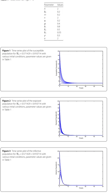
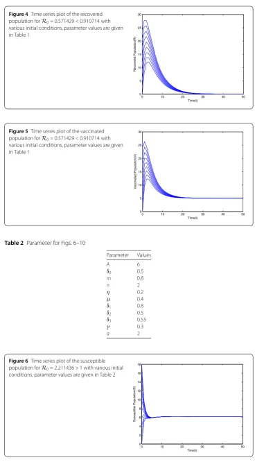
by using the parameter values given in Table 1. Using these parameter values, for differ-ent initial conditions the dynamics of model (5.1) is presdiffer-ented in Figs. 1–5. It shows that system (5.1) has a disease-free equilibrium and it is globally asymptotically stable. This numerical verification supports the result stated in Theorem 3.1.

Table 1 Parameter for Figs. 1–5

Parameter Values

A 2

δ0 0.2

m 0.2

n 2

η 0.2

μ 0.4

δ1 0.8

δ2 0.5

δ3 0.55

γ 0.3

a 2

Figure 1Time series plot of the susceptible population forR0= 0.571429 < 0.910714 with various initial conditions, parameter values are given in Table 1

Figure 2Time series plot of the exposed population for_R0= 0.571429 < 0.910714 with

various initial conditions, parameter values are given in Table 1

Figure 4Time series plot of the recovered population forR0= 0.571429 < 0.910714 with various initial conditions, parameter values are given in Table 1

Figure 5Time series plot of the vaccinated population forR0= 0.571429 < 0.910714 with

various initial conditions, parameter values are given in Table 1

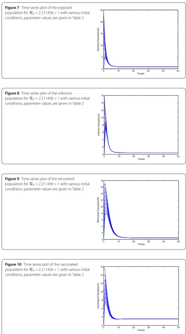
Table 2 Parameter for Figs. 6–10

Parameter Values

A 6

δ0 0.5

m 0.8

n 2

η 0.2

μ 0.4

δ1 0.8

δ2 0.5

δ3 0.55

γ 0.3

a 2

Figure 7Time series plot of the exposed

population forR0= 2.211436 > 1 with various initial conditions, parameter values are given in Table 2

Figure 8Time series plot of the infective

population forR0= 2.211436 > 1 with various initial conditions, parameter values are given in Table 2

Figure 9Time series plot of the recovered population forR0= 2.211436 > 1 with various initial conditions, parameter values are given in Table 2

6 Conclusions

In this paper, we have considered an SVEIR epidemic model with general nonlinear inci-dence rate. In model (1.3), we have divided the total population into five compartments, namely susceptible, exposed, infective, recovered, vaccinated population and investigated the dynamical behavior of this model. Here, we have found that

R0=

δ1 m2(m3+g(0))

∂f

∂I

A m1–_mμη

4

, 0

is a basic reproduction number of system (1.3), which helps us to determine the dynamical behavior of the system. We have showed that system (1.3) to be globally asymptotically stable at disease-free equilibriumP0when

R0< 1 –

Ag(0) –δ0g(A

δ0)

A(m3+g(0)) .

WhenR0> 1, the endemic equilibrium stable both locally and globally has been derived and analyzed under some conditions. The important mathematical findings for the dy-namical behavior of model (1.3) have also numerically been verified for a special case of model (1.3). We would like to point out that the model considered in this paper is not a case study and so it is difficult to choose parameter values from quantitative estimation. We have used hypothetical sets of parameters to verify our analytical results. It is worth to mention that the results presented in this paper improve and extend some related results in [9, 10, 12, 13].

Finally, we remark that there are quite a few spaces to deserve further investigation. For example, we can continue the research in this line considering the vaccination rate

μin our model (1.3) as a continuous function, and, later, a discontinuous function. On the other hand, as is well known, epidemiological models which incorporate the control strategies can be useful to both control the spread of disease and minimize the intervention costs. For our model, it is natural to consider vaccination rate coefficient as a control to reduce the disease burden. Thus, it is important and interesting to prove the existence of optimal control, characterize the optimal control, prove the uniqueness of optimal control, compute the optimal control numerically and investigate how the optimal control depends on various parameters in the models. We will devote to these questions our future work.

Acknowledgements

We would like to thank the editors and referees for their valuable comments and suggestions to improve our paper.

Funding

This work was supported by the National Natural Science Foundation of China (11371015, 11471230, 11671282) and the Natural Science Foundation of Sichuan Provincial Education Department (Grant Nos. 18ZB0581, 14ZB0142) and the Meritocracy Research Funds of China West Normal University (17YC373).

Abbreviations

(SVEIR), Susceptible–Vaccinated–Exposed–Infectious–Recovered.

Availability of data and materials Not applicable.

Competing interests

The authors declare that they have no competing interests.

Consent for publication Not applicable.

Authors’ contributions

All authors contributed equally to this work. All authors read and approved the final manuscript.

Author details

1_{School of Mathematics and Information, China West Normal University, Nanchong, P.R. China.}2_{Department of} Mathematics, Sichuan University, Chengdu, P.R. China.3_{Department of Mathematics and the RINS, Gyeongsang National} University, Jinju, Korea. 4_{School of Management, Sichuan University of Science and Engineering, Zigong, P.R. China.}

Publisher’s Note

Springer Nature remains neutral with regard to jurisdictional claims in published maps and institutional affiliations.

Received: 1 February 2018 Accepted: 16 March 2018

References

1. Naheed, A., Singh, M., Lucy, D.: Numerical study of SARS epidemic model with the inclusion of diffusion in the system. Appl. Math. Comput.229, 480–498 (2014)

2. Billarda, L., Dayananda, P.W.A.: A multi-stage compartmental model for HIV-infected individuals: I waiting time approach. Math. Biosci.249, 92–101 (2014)

3. Upadhyay, R.K., Kumari, N., Rao, V.S.H.: Modeling the spread of bird flu and predicting outbreak diversity. Nonlinear Anal., Real World Appl.9, 1638–1648 (2008)

4. Pongsumpun, P., Tang, I.M.: Dynamics of a new strain of the H1N1 influenza a virus incorporating the effects of repetitive contacts. Comput. Math. Methods Med.2014, Article ID 487974 (2014)

5. Zhou, X., Cui, J.: Analysis of stability and bifurcation for an SEIV epidemic model with vaccination and nonlinear incidence rate. Nonlinear Dyn.63, 639–653 (2011)

6. Kyrychko, Y., Blyuss, K.: Global properties of a delayed SIR model with temporary immunity and nonlinear incidence rate. Nonlinear Anal., Real World Appl.6, 495–507 (2005)

7. Buonomo, B., Lacitignola, D.: Global stability for a four dimensional epidemic model. Note Mat.30, 81–93 (2010) 8. Gumel, A.B., McCluskey, C.C., Watmough, J.: An SVEIR model for assessing potential impact of imperfect anti-SARS

vaccine. Math. Biosci. Eng.3, 485–512 (2006)

9. Khan, M.A., Badshah, Q., Islam, S., et al.: Global dynamics of SEIRS epidemic model with non-linear generalized incidences and preventive vaccination. Adv. Differ. Equ.2015, 88 (2015). https://doi.org/10.1186/s13662-015-0429-3 10. Khan, M.A., Khan, Y., Khan, S., et al.: Global stability and vaccination of an SEIVR epidemic model with saturated

incidence rate. Int. J. Biomath.9, 59–83 (2016). https://doi.org/10.1142/s1793524516500686

11. Liu, X., Yang, L.: Stability analysis of an SEIQV epidemic model with saturated incidence rate. Nonlinear Anal., Real World Appl.13, 2671–2679 (2012)

12. Upadhyay, R.K., Kumari, S., Misra, A.K.: Modeling the virus dynamics in computer network with SVEIR model and nonlinear incident rate. J. Appl. Math. Comput.54, 485–509 (2017)

13. Yang, Y., Zhang, C.M., Jiang, X.Y.: Global stability of an SEIQV epidemic model with general incidence rate. Int. J. Biomath.8, 103–115 (2015). https://doi.org/10.1142/S1793524515500205

14. Zhang, X., Liu, X.N.: Backward bifunction of an epidemic model with saturated treatment. J. Math. Anal. Appl.348, 433–443 (2008)

15. Chidouh, A., Torres, D.: Existence of positive solutions to a discrete fractional boundary value problem and corresponding Lyapunov-type inequalities. Opusc. Math.38, 31–40 (2018)

16. Papageorgiou, N.S., Radulescu, V.D., Repovs, D.D.: Sensitivity analysis for optimal control problems governed by nonlinear evolution inclusions. Adv. Nonlinear Anal.6, 199–235 (2017)

17. Pukach, P., Il’kiv, V., Nytrebych, Z., Vovk, M.: On nonexistence of global in time solution for a mixed problem for a nonlinear evolution equation with memory generalizing the Voigt–Kelvin rheological model. Opusc. Math.37, 735–753 (2017)

18. Xu, R., Ma, Z.: Global stability of a delayed SEIRS epidemic model with saturation incidence rate. Nonlinear Dyn.61, 229–239 (2010)

19. Alexander, M., Moghadas, S.: Bifurcation analysis of an SIRS epidemic model with generalized incidence. SIAM J. Appl. Math.65, 1794–1816 (2005)

20. Bianca, C., Pennisi, M., Motta, S., et al.: Immune system network and cancer vaccine. AIP Conf. Proc.1389, 945–948 (2011). https://doi.org/10.1063/1.3637764

21. Bianca, C., Pappalardo, F., Motta, S., et al.: Persistence analysis in a Kolmogorov-type model for cancer-immune system competition. AIP Conf. Proc.1558, 1797–1800 (2013). https://doi.org/10.1063/1.4825874

22. Cai, L.M., Li, X.Z.: Analysis of a SEIV epidemic model with a nonlinear incidence rate. Appl. Math. Model.33, 2919–2926 (2009)

23. Capasso, V., Serio, G.: A generalization of the Kermack-McKendrick deterministic epidemic model. Math. Biosci.42, 43–61 (1978)

24. Capasso, V.: Global solution for a diffusive nonlinear deterministic epidemic model. SIAM J. Appl. Math.35, 274–284 (1978)

26. Ghergu, M., Radulescu, V.D.: Nonlinear PDEs, Mathematical Models in Biology, Chemistry and Population Genetics. Springer Monographs in Mathematics. Springer, Heidelberg (2012)

27. Dénes, A., Röst, G.: Global stability for SIR and SIRS models with nonlinear incidence and removal terms via dulac functions. Discrete Contin. Dyn. Syst., Ser. B21, 1101–1117 (2016)

28. Hu, Z.X., Bi, P., Ma, W.B., et al.: Bifurcations of an SIRS epidemic model with nonlinear incidence rate. Discrete Contin. Dyn. Syst., Ser. B15, 93–112 (2012)

29. Liu, W., Levin, S.A., Iwasa, Y.: Influence of nonlinear incidence rates upon the behavior of SIRS epidemiological models. J. Math. Biol.23, 187–204 (1986)

30. Ruan, S.G., Wang, W.D.: Dynamical behavior of an epidemic model with a nonlinear incidence rate. J. Differ. Equ.188, 135–163 (2003)

31. Wang, W.D.: Backward bifurcation of an epidemic model with treatment. Math. Biosci.201, 58–71 (2006)

32. Wang, F., Zhang, Y., Wang, C., et al.: Stability analysis of a SEIQV epidemic model for rapid spreading worms. Comput. Secur.29, 410–418 (2010)

33. Xiao, D., Ruan, S.G.: Global analysis of an epidemic model with nonmonotone incidence rate. Math. Biosci.208, 419–429 (2007)

34. Yang, Y., Xiao, D.: Influence of latent period and nonlinear incidence rate on the dynamics of SIRS epidemidogical models. Discrete Contin. Dyn. Syst., Ser. B13, 195–211 (2010)

35. Gao, D.P., Huang, N.J.: A note on global stability for a tuberculosis model. Appl. Math. Lett.73, 163–168 (2017) 36. Gao, D.P., Huang, N.J.: Optimal control analysis of a tuberculosis model. Appl. Math. Model.58, 47–64 (2018) 37. Laarabi, H., Abta, A., Hattaf, K.: Optimal control of a delayed SIRS epidemic model with vaccination and treatment.

Acta Biotheor.63, 87–97 (2015)

38. Wang, W.D., Ruan, S.G.: Bifurcation in an epidemic model with constant removal rate of the infectives. J. Math. Anal. Appl.291, 775–793 (2004)

39. Hale, J.K.: Ordinary Differential Equations, 2nd edn. Krieger, Melbourne (1980)

40. Korobeinikov, A.: Lyapunov functions and global stability for SIR and SIRS epidemiological models with nonlinear transmission. Bull. Math. Biol.30, 615–626 (2006)

41. Brikhoff, G., Rota, G.C.: Ordinary Differential Equations. Ginn, Boston (1982)

42. LaSalle, J.P.: The Stability of Dynamical Systems. Regional Conference Series in Applied Mathematics. SIAM, Philadephia (1976)

43. Kot, M.: Elements of Mathematical Ecology. Cambridge University Press, Cambridge (2001)

44. Li, M.Y., Muldowney, J.S.: On R.A. Smith’s autonomous convergence theorem. Rocky Mt. J. Math.25, 365–378 (1995) 45. Freedman, H.I., Ruan, S.G., Tang, M.X.: Uniform persistence and flows near a closed positively invariant set. J. Differ.

Equ.6, 583–600 (1994)

46. Hutson, V., Schmitt, K.: Permanence and the dynamics of biological systems. Math. Biosci.111, 1–71 (1992) 47. Martin, R.H.: Logarithmic norms and projections applied to linear differential systems. J. Math. Anal. Appl.45, 432–454