ESAIM: PROCEEDINGS,February 2007, Vol.16, 66-76 Eric Canc`es & Jean-Fr´ed´eric Gerbeau, Editors
DOI: 10.1051/proc:2007008
A PROPOSED SIMPLIFICATION OF THE ADAPTIVE LOCAL
DECONVOLUTION METHOD
S. Hickel
1and N.A. Adams
Abstract. The adaptive local deconvolution method (ALDM) [9] provides a systematic framework for the implicit large-eddy simulation (ILES) of turbulent flows. Exploiting numerical truncation errors, the subgrid scale (SGS) model of ALDM is implicitly contained within the discretization. An explicit computation of model terms therefore becomes unnecessary. Subject of the present paper is a modification of the numerical algorithm that allows for reducing the amount of computational operations without affecting the quality of the results. Computational results for isotropic turbulence and plane channel flow show that the simplified adaptive local deconvolution (SALD) method performs similarly to the original method ALDM and at least as well as established explicit models.
1.
Introduction
In Large-Eddy Simulation (LES) of turbulent flows the evolution of non-universal larger scales is computed,
whereas their interaction with unresolved subgrid scales (SGS) is modeled. SGS effects are modeledexplicitly if
the underlying conservation law is modified and subsequently discretized. The filtering concept of Leonard [14] is commonly employed for deriving explicit SGS models without reference to a computational grid and without taking into account a discretization scheme. However, numerically computed SGS stresses are strongly affected by the truncation error of the discretization scheme [6]. This interference can result in strange results such as the lack of grid convergence. Employing an explicit SGS model, Schumann [19] already argued that discretization effects should be taken into account within the SGS model formulation.
AsImplicit Large-Eddy Simulation (ILES) we denote the situation when the unmodified conservation law is
discretized and the numerical truncation error acts as SGS model. Since the SGS model isimplicitly contained
within the discretization scheme an explicit computation of model terms becomes unnecessary.
One recent approach, the Adaptive Local Deconvolution Method (ALDM) [9], provides a systematic frame-work for implicit SGS modeling in turbulent flows. With ALDM numerical discretization and SGS modeling are merged entirely. A local reconstruction of the solution is obtained from a solution-adaptive combination of deconvolution polynomials. Free parameters, involved in the non-linear weight functions of the respective contributions, allow for SGS modeling. Optimal model parameters were determined by systematically minimiz-ing a cost function which measures the difference between spectral numerical viscosity of ALDM and the eddy viscosity from EDQNM theory for isotropic turbulence so that the truncation error has physical significance.
The efficiency of this approach was demonstrated in Ref. [1] for 1D conservation laws on the example of the viscous Burgers equation. The extension to three spatial dimensions and the incompressible Navier-Stokes equations is detailed in Ref. [9]. ALDM has proven itself as a reliable, accurate, and efficient method for LES of three-dimensional homogeneous isotropic turbulence [9], for plane channel flow [11], and for the complex
1 Institute of Aerodynamics, Technische Universit¨at M¨unchen, D-85747 Garching, Germany. E-mail: [email protected] c
EDP Sciences, SMAI 2007
flow in a channel with periodic constrictions [2, 13]. All simulations show good agreement with theory and experimental data and thus demonstrate the good performance of the implicit model. It has been shown that ALDM performs at least as well as established explicit models.
In the present paper we revisit the numerical formulation of ALDM for the incompressible 3D Navier-Stokes equations. A simplification of the method is proposed. The good performance of the implicit model is preserved while computational costs are reduced significantly.
2.
Solution-adaptive local deconvolution revisited
ALDM is a general nonlinear, i.e. solution adaptive, discretization scheme designed for implicit LES. It is based on standard approaches which were modified in such a way that the resulting truncation error functions as implicit SGS model. In the following, all relevant parts of the algorithm are reviewed. We demonstrate how the original formulation of ALDM [9] can be further simplified to accelerate computation. The reader is
provided with a self-contained paper on thesimplified adaptive local deconvolution (SALD) method.
The incompressible Navier-Stokes equations in non-dimensional form read
∂u
∂t +∇·F(u) +∇p−ν∇·∇u=0, (1a)
∇·u= 0, (1b)
whereuis the velocity vector,pis the pressure, andν is the kinematic viscosity. For implicit modeling we only
consider the nonlinear term ∇·F +∇pin the momentum equation (1a), whereas the linear terms, i.e. the
diffusive flux, are approximated by a standard centered discretization. ALDM applies to the convective flux
F = uu. For incompressible flows a fractional-step approach is taken where the normal stresses due to the
pressurepare subsequently computed by solving a Poisson equation.
Even if filtering is not performed explicitly we can use the filtered formulation of Leonard [14] as analytical tool when designing and analyzing discrete operators
∂uN
∂t +G∗∇·FN(G
−1∗u
N) +∇p−ν∇·∇uN =−G∗∇·τSGS , (2a)
∇·uN = 0. (2b)
Note that with implicit LES the subgrid-stress tensorτSGSis not computed explicitly but modeled by numerical
truncation errors.
A finite-volume discretization is based on the top-hat filter kernel
G(xi,j,k,x) =
1 ΔxiΔyjΔzk
1 ,(xi,j,k+x)∈Ii,j,k
0 , otherwise , (3)
which returns the cell average of a function
ϕ(xi,j,k, t) = 1 ΔxiΔyjΔzk
Ii,j,k
where the integration domain Ii,j,k = [xi−1
2, xi+12]×[yj−12, yj+12]×[zk−12, zk+12] is equivalent to a cell of the underlying Cartesian computational grid so that the filter width corresponds to the local grid size
Δxi,j,k= ⎡ ⎢ ⎢ ⎣
Δxi
Δyj
Δzk ⎤ ⎥ ⎥ ⎦= ⎡ ⎢ ⎢ ⎣
xi+1/2−xi−1/2 yj+1/2−yj−1/2 zk+1/2−zk−1/2 ⎤ ⎥ ⎥
⎦ . (5)
Here and in the following half-integer indices denote cell faces and the coordinate system{x , y , z}is
synony-mous with{1,2,3}. The 3D filter kernel Gcan be factorized into three 1D operators
G(x) =Gx(x)∗Gy(y)∗Gz(z). (6)
An inverse-filter operation can be defined as convolution with the inverse kernels
G−1(x) =G−1
x (x)∗G−y1(y)∗G−z1(z). (7)
In the framework of a finite-volume discretization filtering applied to the flux divergence returns the flux through the surfaceSi,j,kof cellIi,j,k. By Gauss’ theorem we obtain
G∗∇·F G−1∗u
i,j,k =
1
Δxi Gy∗Gz∗
1
f(G−1∗u)
i+12,j,k− 1
f(G−1∗u)
i−12,j,k
+ 1
Δyj Gz∗Gx∗
2
f(G−1∗u)
i,j+12,k− 2
f(G−1∗u)
i,j−12,k
+ 1
Δzk Gx∗Gy∗
3
f(G−1∗u)
i,j,k+12 − 3
f(G−1∗u)
i,j,k−12
, (8)
where the flux vectorlf =ulu denotes thel-direction component of F. As a consequence of this identity (8),
finite-volume schemes require a reconstruction of data at the faces of the computational volumes. The numerical computation of eq. (8) necessarily involves approximations
G∗∇ ·FG−1∗u
i,j,k≈
G∗∇·FG−1∗u
i,j,k (9)
The original formulation of ALDM [9] employs a standard Gaussian quadrature rule with kernelCk and order
OΔxk
to approximate the filter operationGl∗Gmover the cell face transversal to the flux direction whereas
a solution adaptive deconvolution scheme is proposed to approximateG−1. In Ref. [9] a simple second-order
accurate filtering scheme is used forGl∗Gm. The benefits of higher-order schemes were found to be negligible
since second-order accurate interpolants contribute to the deconvolution operator.
Recent numerical experiments presented in the following section have shown that also the deconvolution scheme can be simplified significantly without affecting the prediction power of the implicit SGS model. Based on these results we recommend as simplification
G∗∇ ·FG−1∗u
i,j,k =
1 Δxi
1 fG−1
x ∗u i+12,j,k
−1fG−1
x ∗u i−12,j,k
+ 1
Δyj
2 fG−1
y ∗u i,j+12,k
−2fG−1
y ∗u i,j−12,k
+ 1
Δzk
3 fG−1
z ∗u i,j,k+12
−3fG−1
z ∗u i,j,k−12
where no filteringGl∗Gmis applied. Furthermore, approximate deconvolutionG−l 1is performed only in those directionslfor which interpolation at cell faces is necessary using the 1D reconstruction (i.e. deconvolution and
interpolation) operatorXλ
x of ALDM proposed in Ref. [1] and adapted in Ref. [9]. In the simplified adaptive
local deconvolution method the fully 3D scheme of ALDM is replaced by a single 1D step at the target cell face. Deconvolution is not performed in the transverse directions.
In the following we repeat the derivation of the algorithm as given in Ref. [9] and point out the differences
between full ALDM and the SALD method. The 1D adaptive deconvolution operator, denoted byXλ
x, is
de-fined on a 1D gridxN ={xi}. Applied to the filtered grid functionϕN ={ϕ(xi)}it returns the approximately
deconvolved grid functionϕλ
N =. {ϕ(xi+λ)}on the shifted gridxλN ={xi+λ} Xλ
xϕN ={ϕ(ϕ, x i+λ) +O(Δxiκ)}=ϕλN . (11)
Following eq. (7), a 3D reconstruction is obtained by successive 1D operations
ϕλN =Xλ ϕN =Xzλ3
Xλ2 y
Xλ1
x ϕN . (12)
The filtered data are given at the cell centers{xi}. Reconstruction at the left cell faces{xi−1
2} is indicated by
λ=−1/2 and at the right faces{xi+1
2} byλ= +1/2. The ALDM operators which perform deconvolution at
the cell centers, denoted byλ= 0, are replaced by identity in the simplified algorithm.
Deconvolution and interpolation are done simultaneously using Lagrangian interpolation polynomials as proposed by Hartenet al.[8]. Given a generick-point stencil ranging fromxi−r toxi−r+k−1 the 1D ansatz for
the top-hat kernel (3) reads
ϕ(xi+λ) = k−1
l=0
cλk,r,l(xi)ϕN(xi−r+l) +O
Δxik
, (13)
withr∈ {0, . . . , k}. The grid-dependent coefficients are
cλk,r,l(xi) =
xi−r+l+12 −xi−r+l−12
k
m=l+1 k p=0 p=m
k n=0 n=p,m
xi+λ−xi−r+n−1 2
k n=0
n=m
xj−r+m−12 −xi−r+n−12
, (14)
as given by Shu [21]. They apply for grids with variable mesh width and for arbitrary target positionsxi+λ. In
case of a staggered grid the values ofxi are different for each velocity component and the coefficientscλk,r,lhave
to be specified accordingly.
Selecting a particular interpolation stencil would return a linear discretization with a fixed, solution
inde-pendent functional expression of thek-th order truncation error, provided the function is sufficiently smooth on
the interpolation stencil. ALDM adopts the idea of the Weighted-Essentially-Non-Oscillatory (WENO) scheme
of Shu [21] where interpolation polynomials of a single orderk≡Kare selected and combined nonlinearly. The
essential difference between ALDM and WENO is that we superpose all interpolants of orderk= 1, . . . , K
ϕλN(xi+λ) = K
k=1
k−1
r=0
ωk,rλ (ϕN, xi) k−1
l=0
cλk,r,l(xi)ϕN(xi−r+l) (15)
to allow for lower-order contributions to the truncation error for implicit SGS modeling [1]. Usually it isK= 3.
The weights ωλ
smooth regions [21]. For our purpose, however, we do not need highest possible order of accuracy. Rather the superposition (15) introduces free discretization parameters which allow to control error cancelations. The sum of all weights is constrained to be unity for consistency. More restrictively we require
ωk,rλ (ϕN, xi) =
1
K γλ
k,rβk,r(ϕN, xi) k−1
s=0γ
λ
k,sβk,s(ϕN, xi)
, (16)
withr = 0, . . . , k−1 for each k = 1, . . . , K . Note thatλdenotes a superscript index and not a power. The solution-adaptive behavior of ALDM is controlled by the functional
βk,r(ϕN, xi) =
εβ+ k−r−2
m=−r
ϕi+m+1−ϕi+m 2
−2
, (17)
whereεβ is a small number to prevent division by zero in eq. (16). βk,r measure the smoothness of the grid
function on the respective stencil to obtain a non-linear adaptation of the deconvolution. The advantage of
definition (17) over smoothness measures proposed by Liuet al. [17] and by Jiang & Shu [12] is that
βk,r(ϕN, xi) =βk,r−1(ϕN, xi−1) . (18)
can be exploited to improved computational efficiency. The parametersγλ
k,r represent a stencil-selection
pref-erence that would become effective in the statistically homogeneous case. The requirement of an isotropic discretization for this case implies symmetries on the parameters
γk,r−1/2=γk,k+1/−21−r. (19)
The number of independent parameters is further reduced by the consistency requirementkr−=01γ+1k,r/2 = 1. Using the simplified procedure with K = 3, three parameters { γ2+1,0/2 , γ+1
/2 3,0 , γ+1
/2
3,1 } remain available
for modeling. The original formulation [9] provides one additional parameterγ30,1. Optimal parameters for the
original scheme were found by means of an evolutionary optimization algorithm [1, 9, 10]. These parameters, reproduced in table 1, result in an excellent spectral match of the numerical viscosity of ALDM with prediction of EDQNM theory [3, 15]. We have refrained from repeating the parameter optimization with the simplified scheme because the change by applying the transversal deconvolution operation was found to be negligible in terms of the effective numerical viscosity. For further computational details of evaluation and optimization of the spectral numerical viscosity of ALDM the reader should refer to Ref. [9].
Table 1. Optimized values for discretization parameters [9].
parameter γ2+1,0/2 γ
+1/2
2,1 γ
+1/2
3,0 γ
+1/2
3,1 γ
+1/2
3,2 σ
optimal value 1.00000 0.00000 0.01902 0.08550 0.89548 0.06891
It is interesting to note that the evolutionary optimization finally selectedγ2+1,0/2 = 1 andγ
+1/2
2,1 = 0.
Another tool which is exploited is the choice of an appropriate and consistent numerical flux function that approximates the physical flux function
FN ≈F =uu and l∼
f ≈lf =ulu. (20)
A review of common numerical flux functions can be found, e.g., in LeVeque’s textbook [16]. During construction of ALDM the modified differential equations (MDE) of various flux functions were analyzed [1]. Based on these findings the following modification of a Lax-Friedrichs flux function was proposed [9] for the three-dimensional Navier-Stokes equations and collocated Cartesian grids
1∼ fi+1
2,j,k =
1 4
uiL+1,j,k+uRi,j,k uLi+1,j,k+uRi,j,k −1 σi,j,k ⎡ ⎢ ⎢ ⎣
|ui+1,j,k−ui,j,k|(uLi+1,j,k−uRi,j,k) |vi+1,j,k−vi,j,k|(viL+1,j,k−vRi,j,k) |wi+1,j,k−wi,j,k|(wLi+1,j,k−wi,j,kR )
⎤ ⎥ ⎥
⎦ , (21a)
2∼ fi,j+1
2,k=
1 4
vi,jB+1,k+vFi,j,k uBi,j+1,k+uFi,j,k −2 σi,j,k ⎡ ⎢ ⎢ ⎣
|ui,j+1,k−ui,j,k|(uBi,j+1,k−uFi,j,k) |vi,j+1,k−vi,j,k| (vBi,j+1,k−vFi,j,k) |wi,j+1,k−wi,j,k|(wBi,j+1,k−wi,j,kF )
⎤ ⎥ ⎥
⎦ , (21b)
3∼ fi,j,k+1
2 =
1 4
wi,j,kD +1+wUi,j,k uDi,j,k+1+uUi,j,k −3 σi,j,k ⎡ ⎢ ⎢ ⎣
|ui,j,k+1−ui,j,k|(uDi,j,k+1−uUi,j,k) |vi,j,k+1−vi,j,k| (vDi,j,k+1−vUi,j,k) |wi,j,k+1−wi,j,k|(wDi,j,k+1−wi,j,kU )
⎤ ⎥ ⎥
⎦ . (21c)
A further simplification of this flux function is not possible without affecting the performance of the model. However, the computational efficiency can be improved by merging convective and diffusive flux computations. The extension to a staggered grid arrangement is straight forward and leads to
1∼ fi+1
2,j,k=
1 4 ⎡ ⎢ ⎢ ⎣
(uLi+1,j,k+uRi,j,k) (uLi+1,j,k+uRi,j,k)
(uB
i,j+1,k+uFi,j,k) (viL+1,j,k+vRi,j,k)
(uD
i,j,k+1+uUi,j,k) (wiL+1,j,k+wRi,j,k) ⎤ ⎥ ⎥ ⎦−1σi,j,k
⎡ ⎢ ⎢ ⎣
|ui+1,j,k−ui,j,k|(uLi+1,j,k−uRi,j,k) |vi+1,j,k−vi,j,k|(vLi+1,j,k−vi,j,kR ) |wi+1,j,k−wi,j,k|(wLi+1,j,k−wRi,j,k)
⎤ ⎥ ⎥
⎦ , (22a)
2∼ fi,j+1
2,k=
1 4 ⎡ ⎢ ⎢ ⎣
(vL
i+1,j,k+vi,j,kR ) (uBi,j+1,k+uFi,j,k)
(vB
i,j+1,k+vFi,j,k) (vi,jB+1,k+vi,j,kF )
(vD
i,j,k+1+vi,j,kU ) (wBi,j+1,k+wi,j,kF ) ⎤ ⎥ ⎥ ⎦−2σi,j,k
⎡ ⎢ ⎢ ⎣
|ui,j+1,k−ui,j,k|(uBi,j+1,k−uFi,j,k) |vi,j+1,k−vi,j,k|(vi,jB+1,k−vi,j,kF ) |wi,j+1,k−wi,j,k|(wi,jB+1,k−wFi,j,k)
⎤ ⎥ ⎥
⎦ , (22b)
3∼ fi,j,k+1
2 = 1 4 ⎡ ⎢ ⎢ ⎣
(wL
i+1,j,k+wi,j,kR ) (uDi,j,k+1+uUi,j,k)
(wBi,j+1,k+wi,j,kF ) (vDi,j,k+1+vi,j,kU )
(wD
i,j,k+1+wi,j,kU ) (wDi,j,k+1+wUi,j,k) ⎤ ⎥ ⎥ ⎦−3σi,j,k
⎡ ⎢ ⎢ ⎣
|ui,j,k+1−ui,j,k| (uDi,j,k+1−uUi,j,k) |vi,j,k+1−vi,j,k|(vi,j,kD +1−vi,j,kU ) |wi,j,k+1−wi,j,k|(wi,j,kD +1−wi,j,kU )
⎤ ⎥ ⎥
⎦ . (22c)
Table 2. Interpolation directions for 3D reconstruction.
Direction Example
(R) rightward uR
i,j,k≈u(xi+12, yj, zk)
(L) leftward uLi,j,k≈u(xi−1
2, yj, zk)
(F) forward uF
i,j,k≈u(xi, yj+1
2, zk)
(B) backward uB
i,j,k≈u(xi, yj−12, zk)
(U) upward uU
i,j,k≈u(xi, yj, zk+1
2)
(D) downward uD
i,j,k≈u(xi, yj, zk−12)
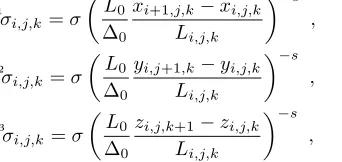
function. For developed turbulence the Kolmogorov theory predicts a scaling with a 1/3 power of the two-point
separation [5]. The coefficients
1
σi,j,k=σ
L0
Δ0
xi+1,j,k−xi,j,k Li,j,k
−s
, (23a)
2
σi,j,k=σ
L0
Δ0
yi,j+1,k−yi,j,k Li,j,k
−s
, (23b)
3
σi,j,k=σ
L0
Δ0
zi,j,k+1−zi,j,k Li,j,k
−s
, (23c)
were introduced to compensate for varying grid-size effects. The scalar factorσ adds another free parameter
to ALDM, see table 1. For isotropic turbulence it was found thats = 1/3 ensures a resolution-independent
numerical viscosity, as long as the numerical cutoff is located within the inertial range of the kinetic-energy
spectrum. Δ0 = 2π/32 is a reference grid size as in Ref. [9]. The original scheme for isotropic turbulence is
recovered ifLi,j,k=L0. For the purpose of wall modeling a van Driest damping is introduced
Li,j,k=L0−L0exp
−
lW uτ a ν
d
, (24)
where lW is the wall distance and uτ is the friction velocity at the closest wall, dand a are free parameters.
During computational experimentation only a weak dependence between these parameters and the prediction
quality could be found. We estimate optimal values as d = s−1 and a = 25 based on these computational
experiments. The proposed van Driest damping reduces the SGS dissipation at wall distances below 50ν/uτ,
whereas the scheme remains unchanged above. The friction velocity is defined as
uτ(x) =
ν∂u(x) ∂nW(x)
. (25)
The derivative is evaluated at the wall using the wall-normal unit vector nW. In plane channel flow it is
convenient to compute the friction velocity from
uτ= ν
h Reτ (26)
approximating the unknown Reynolds numberReτ by its nominal value.
In order to allow for the treatment of arbitrarily shaped walls and moving obstacles a level-set based approach
scalar quantity within the entire fluid domain. The interior of solid obstacles being marked by a negative sign
oflW. The wall-normal unit vector is obtained from the gradient of the level-set function
nW =|∇∇lW lW|
(27)
presuming the level-set functionlW to be smooth. Since it is lim
lW→0|∇lW|
= 1, the local wall-tangential friction
velocity can be evaluated as
uτ(x) =
ν|∇lW(x)·∇u(x)| (28)
in the near-wall region.
3.
Numerical results
In this section computational results for LES of decaying isotropic turbulence and turbulent channel flow are presented for validation of the proposed method. SALD and ALDM are implemented in an experimental flow solver, INCA, which solves the incompressible Navier-Stokes equations in Cartesian coordinates. This solver is our workhorse for numerical-method development and covers various linear and nonlinear discretizations on collocated and staggered grids as well as spectral methods.
For time advancement, we employ the explicit 3rd-order Runge-Kutta scheme of Shu [7, 20]. This
time-discretization scheme is total-variation diminishing (TVD) for Courant numbers CFL ≤1, provided the
un-derlying spatial discretization is TVD. We use CFL = 1.0 for all simulations. Pressure-Poisson equation and
diffusive term are discretized by 2nd-order centered differences. In order to enhance computational efficiency, the discretized diffusive term is merged with the convective-flux approximation, eq. (21-22). Periodic boundary conditions allow to use a fast FFT-based Poisson solver with appropriate modified wave numbers for the first test case, where oddball modes are removed in spectral space. The pressure-Poisson solver for the channel-flow test case employs FFT in streamwise and spanwise direction and performs direct tridiagonal-matrix inversions in wall-normal direction. It should be noted that the oddball modes remain part of the solution and a staggered velocity arrangement is used for the second test case.
3.1.
Homogeneous isotropic turbulence
As a first test case the numerical schemes are applied to decaying grid-generated turbulence. The computa-tions are initialized with energy spectrum and Reynolds numbers adapted to the wind-tunnel experiments of Comte-Bellot and Corrsin [4], denoted hereafter as CBC. Among other space-time correlations CBC provides streamwise energy spectra for grid-generated turbulence at three positions downstream of a mesh. Table 3 of Ref. [4] gives corresponding 3D energy spectra which were obtained under the assumption of isotropy.
In the simulation this flow is modeled as decaying turbulence in a (2π)3-periodic computational domain,
discretized on a collocated grid with 643 cells. Based on the Taylor hypothesis the temporal evolution in the
simulation corresponds to a downstream evolution in the wind-tunnel experiment with the experimental mean-flow speed which is approximately constant. The energy distribution of the initial velocity field is matched to the first measured 3D energy spectrum of CBC. The SGS model is verified by comparing computational and experimental 3D energy spectra at later time instants which correspond to the other two measuring stations. For more details, particularly with regard to non-dimensionalization and initial-data generation, we refer to [9].
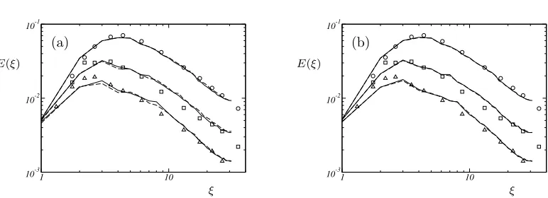
We present numerical results from implicit LES with the original ALDM scheme of Hickelet al.[9] and with
successively simplified formulations proposed in the present paper. Figure 1a compares results obtained by
4th-order (C4) with those obtained by a second order (C2) Gaussian quadrature rule for the approximation of
the filter operationGl∗Gm. It is found that the choice of the integration kernel has negligible effects on the
1 10
10-3
10-2
10-1
(a)
E(ξ)
ξ
1 10
10-3
10-2
10-1
(b)
E(ξ)
ξ
Figure 1. Instantaneous 3D energy spectra for LES with 643 cells of the Comte-Bellot –
Corrsin experiment. (a)−−−−−−− ALDM with full deconvolution andC2,−−−−ALDM with
full deconvolution andC4. (b)−−−−−−−SALD,−−−−ALDM with full deconvolution andC2.
Symbols represent experimental data of Ref. [4].
3.2.
Turbulent channel flow
As an example for anisotropic wall bounded turbulence, we simulate channel flow at Rebulk = 6875 (Reτ =
395). Reference DNS data are provided by Moseret al.[18]. The computational domain measures 2πh×2h×πh
(streamwise × wall-normal × spanwise), where h is the channel half width. The spectral DNS of Moser et
al.required 256×193×192 grid points, whereas the computational grid of the present LES consists of 64×68×64 cells. To accommodate the change of turbulence structure in the vicinity of solid walls, the grid is stretched in wall-normal direction
y(j) =− 1 tanh (CG)
tanh
CG−2CG j Ny+ 1
, (29)
whereNy is the number of cells in the wall-normal direction andCG= 2.0 is the grid-stretching parameter.
Figure 2 shows profiles of mean velocity, Reynolds stresses, mean pressure, and pressure fluctuations from LES with the original and the simplified scheme. We observe a close match between both simulations and a good agreement with the reference DNS data. Inevitable differences between DNS and LES become most evident in the pressure fluctuations. Note the correct wall-asymptotic behavior of the Reynolds stresses of the LES. These results are encouraging and show that the implicit modeling approach gives good results for low-Reynolds-number wall-bounded flows although the model parameters were derived for isotropic turbulence and high Reynolds numbers.
4.
Conclusion
In the present paper we have revised the numerical algorithm of the Adaptive Local Deconvolution Method (ALDM) for the incompressible 3D Navier-Stokes equations. We have given recommendations for the efficient implementation of ALDM. A simplification of the algorithm is proposed leading to the simplified adaptive local deconvolution (SALD) method. The resulting SALD method allows for considerable savings of computational resources. It is about twice as fast as the original ALDM, whereas the prediction power of the implicit model is preserved. The method is more efficient than a second-order central scheme with a dynamic Smagorinsky SGS model, in particular with regard to CPU time. Note that ALDM gives at least as good predictions as established explicit models [9].
-1,0 -0,8 -0,6 -0,4 -0,2 0,0 0,0
0,4 0,8 1,2
u
/Ubu
lk
y/h 10
-1
100 101 102
0 4 8 12 16 20 24
u
/Uτ
y/l+
-1,0 -0,8 -0,6 -0,4 -0,2 0,0
0,00 0,01 0,02 0,03
u
ui /Ui 2 bulk
y/h
0 20 40 60 80
0 2 4 6 8 10
u
ui /Ui 2 τ
y/l+
-1,0 -0,8 -0,6 -0,4 -0,2 0,0
-0,003 -0,002 -0,001 0
u
u1 /U2 2 bulk
y/h
0 20 40 60 80
-1 -0,8 -0,6 -0,4 -0,2 0
u
u1 /U2 2 τ
y/l+
-1,0 -0,8 -0,6 -0,4 -0,2 0,0
-4×10⁻³
-3×10⁻³
-2×10⁻³
-1×10⁻³
0
p
/U
2 bulk
y/h
-1,00 -0,8 -0,6 -0,4 -0,2 0,0
4×10⁻⁵
8×10⁻⁵
p
p /U 4 bulk
y/h
Figure 2. Mean profiles of velocity and pressure, Reynolds stresses, and pressure fluctuations
for LES of turbulent channel flow at Reτ = 395. −−−−−−− SALD , −−−− ALDM with full
of the convective term is relevant. This holds in particular for flow configurations where efficient FFT-based solvers for the pressure-Poisson equation are available, such as homogeneous turbulence and channel flow.
References
[1] N.A. Adams, S. Hickel, and S. Franz. Implicit subgrid-scale modeling by adaptive deconvolution.J. Comp. Phys., 200:412–431, 2004.
[2] N.A. Adams, S. Hickel, T. Kempe, and J.A. Domaradzki. On the relation between subgrid-scale modelling and numerical discretization in large-eddy simulation. InProceedings of the Cyprus International Symposium on Complex Effects in Large Eddy Simulations (CY-LES2005), Limassol, Cyprus, 2005.
[3] J.-P. Chollet. Two-point closures as a subgrid-scale modeling tool for large-eddy simulations. In F.Durst and B.E. Launder, editors,Turbulent Shear Flows IV, pages 62–72, Heidelberg, 1984. Springer.
[4] G. Comte-Bellot and S. Corrsin. Simple Eulerian time correlation of full and narrow-band velocity signals in grid-generated ‘isotropic’ turbulence.J. Fluid Mech., 48:273–337, 1971.
[5] U. Frisch.Turbulence. Cambridge University Press, 1995.
[6] S. Ghosal. An analysis of numerical errors in large-eddy simulations of turbulence.J. Comput. Phys., 125:187–206, 1996. [7] S. Gottlieb and C.-W. Shu. Total variation diminishing Runge-Kutta schemes.Math. Comput., 67:73–85, 1998.
[8] A. Harten, B. Engquist, S. Osher, and S. Chakravarthy. Uniformly high order accurate essentially non-oscillatory schemes, III. J. Comp. Phys., 71:231–303, 1987.
[9] S. Hickel, N.A. Adams, and J.A. Domaradzki. An adaptive local deconvolution method for implicit LES. J. Comp. Phys., 213:413–436, 2006.
[10] S. Hickel, S. Franz, N.A. Adams, and P.D. Koumoutsakos. Optimization of an implicit subgrid-scale model for LES. In Proceedings of the 21st International Congress of Theoretical and Applied Mechanics (ICTAM), Warsaw, Poland, 2004. [11] S. Hickel, T. Kempe, and N.A. Adams. On implicit subgrid-scale modeling in wall-bounded flows. In Proceedings of the
EUROMECH Colloquium 469, pages 36–37, Dresden, Germany, 2005.
[12] G.-S. Jiang and C.-W. Shu. Efficient implementation of weighted ENO schemes.J. Comput. Phys., 126:202–228, 1996. [13] T. Kempe, S. Hickel, and N.A. Adams. LES of the flow over periodic hills using implicit subgrid scale modeling. InERCOFTAC
Fluid Dynamics Colloquium, Prague, Czech Republic, 2005.
[14] A. Leonard. Energy cascade in large eddy simulations of turbulent fluid flows.Adv. Geophys., 18A:237–248, 1974. [15] M. Lesieur.Turbulence in Fluids. Kluwer Academic Publishers, Dordrecht, The Netherlands, 3 edition, 1997. [16] R. J. LeVeque.Numerical methods for conservation laws. Birkh¨auser, Basel, Switzerland, 1992.
[17] S. W. Liu, C. Meneveau, and J. Katz. On the properties of similarity subgrid-scale models as deduced from measurements in a turbulent jet.J. Fluid Mech., 275:83–119, 1994.
[18] R. D. Moser, J. Kim, and N.N. Mansour. Direct numerical simulation of turbulent channel flow up to Reτ= 590.Phys. Fluids, 11:943–945, 1999.
[19] U. Schumann. Subgrid scale model for finite-difference simulations of turbulence in plane channels and annuli.J. Comp. Phys., 18:376–404, 1975.
[20] C.-W. Shu. Total-variation-diminishing time discretizations.SIAM J. Sci. Stat. Comput., 9(6):1073–1084, 1988.
![Table 1. Optimized values for discretization parameters [9].](https://thumb-us.123doks.com/thumbv2/123dok_us/10086512.1995221/5.595.128.459.599.641/table-optimized-values-for-discretization-parameters.webp)