www.geosci-model-dev.net/4/591/2011/ doi:10.5194/gmd-4-591-2011
© Author(s) 2011. CC Attribution 3.0 License.
Geoscientific
Model Development
Coupled atmosphere-wildland fire modeling with WRF 3.3 and
SFIRE 2011
J. Mandel1, J. D. Beezley1, and A. K. Kochanski2
1Department of Mathematical and Statistical Sciences, University of Colorado Denver, Denver, CO, USA 2Department of Meteorology, University of Utah, Salt Lake City, UT, USA
Received: 5 February 2011 – Published in Geosci. Model Dev. Discuss.: 9 March 2011 Revised: 17 June 2011 – Accepted: 28 June 2011 – Published: 7 July 2011
Abstract. We describe the physical model, numerical algo-rithms, and software structure of a model consisting of the Weather Research and Forecasting (WRF) model, coupled with the fire-spread model (SFIRE) module. In every time step, the fire model inputs the surface wind, which drives the fire, and outputs the heat flux from the fire into the atmo-sphere, which in turn influences the atmosphere. SFIRE is implemented by the level set method, which allows a sub-mesh representation of the burning region and a flexible im-plementation of various kinds of ignition. The coupled model is capable of running on a cluster faster than real time even with fine resolution in dekameters. It is available as a part of the Open Wildland Fire Modeling (OpenWFM) environ-ment at http://openwfm.org, which contains also utilities for visualization, diagnostics, and data processing, including an extended version of the WRF Preprocessing System (WPS). The SFIRE code with a subset of the features is distributed with WRF 3.3 as WRF-Fire.
1 Introduction 1.1 Background
Wildland fires impact the lives of millions of people and cause major damage every year worldwide, yet they are a natural part of the cycle of nature. Better tools for modeling wildland fire behavior are important for managing fire sup-pression, planning controlled burns to reduce the fuels, as
Correspondence to: J. Mandel ([email protected])
well as to help assess fire danger. Fire models range from tools based on Rothermel (1972) fire spread rate formulas, such as BehavePlus (Andrews, 2007) and FARSITE (Finney, 1998), suitable for operational forecasting, to sophisticated 3-D computational fluid dynamics and combustion simula-tions suitable for research and analysis, such as FIRETEC (Linn et al., 2002) and WFDS (Mell et al., 2007). Behave-Plus, the PC-based successor of the calculator-based BE-HAVE, determines the fire spread rate at a single point from fuel and environmental data, FARSITE uses the fire spread rate to provide operation 2-D simulation on a PC, while sim-ulations of wildfires spreading across areas of tens of kilo-meters performed using FIRETEC or WFDS run slower than real time, even if executed on a parallel supercomputer.
reproducing qualitatively the general wildland fire shape re-sults from the two-way interaction between the fire and the atmosphere (Clark et al., 1996a,b, 2004; Coen, 2005). 1.2 Development of the coupled model code
The coupled WRF and SFIRE code (Mandel et al., 2009) combines the Weather Research and Forecasting Model (WRF) with the ARW dynamical core (Skamarock et al., 2008) with a semi-empirical fire spread model. It is in-tended to be faster than real time in order to deliver a fore-cast. The code has grown out of the NCAR’s CAWFE code (Clark et al., 1996a,b, 2004; Coen, 2005). CAWFE con-sists of the Clark-Hall mesoscale atmospheric model, cou-pled with a tracer-based fire spread model. Although the Clark-Hall model has many good properties, it is a legacy serial code, not supported, and difficult to modify or use for real cases requiring real meteorological data, topography, and fuel maps, while WRF is a parallel supported commu-nity code routinely used for real runs. See Coen and Patton (2010) for a further discussion of their relative merits in the wildland fire application. The model was started as WRF-Fire by Patton and Coen (2004), who proposed a combination of WRF with the tracer-based model from CAWFE, formu-lated a road map, and made the important observation that the innermost domain of the weather code, which interacts directly with the fire model, needs to run in the Large Eddy Simulation (LES) mode. Patton ported the Fortran 77-based fire module from CAWFE to Fortran 90 and developed the initial coupled code with WRF, with the fire model running on a finer mesh than the atmospheric model, and interpola-tions between the two. However, instead of using the exist-ing tracer-based CAWFE code, the fire module SFIRE was developed based on the level set method (Osher and Fed-kiw, 2003). A more complete timeline is available at http: //www.openwfm.org/wiki/OpenWFM development notes.
One of the reasons for replacing the fire propagation scheme was that the representation of the fire region by the level set function was thought to be more flexible than the representation of the burning region in CAWFE by four trac-ers in each cell of the fire mesh. In particular, the level set function can be manipulated more easily than tracers for the purpose of data assimilation. (Note that the tracers are related to particles, used in computational fluid dynamics, and they represent a Lagrangian approach, while the level set method is an Eulerian approach.) Insertion of the heat fluxes, while fundamentally the same as in CAWFE, had to be redone for WRF variables already in Patton’s initial code. Thus, only the code for the calculation of the fire spread rate and the heat fluxes remained from CAWFE.
While SFIRE takes advantage of the experience accumu-lated with CAWFE, WRF is quite different from the Clark-Hall atmospheric model and the fireline propagation algo-rithm in SFIRE is also different. Thus, it needs to be demon-strated that WRF coupled with SFIRE can deliver similar
results as CAWFE, and the coupled model needs to be vali-dated against real fires (Sect. 9).
1.3 Other related work
The level set method was used for a surface fire spread model in Mallet et al. (2009). Filippi et al. (2009) coupled the at-mospheric model Meso-nh with fire propagation by tracers. Tiger (Mazzoleni and Giannino, 2010) uses a 2-D combu-sion model based on reaction-convection-diffucombu-sion equations and a convection model to emulate the effect of the fire on the wind. FIRESTAR (Morvan and Dupuy, 2004) is a phys-ically accurate wildland fire model in two dimensions, one horizontal and one vertical. UU LES-Fire (Sun et al., 2009) couples the University of Utah’s Large Eddy Simulation code with the tracer-based code from CAWFE. See the survey by Sullivan (2009) for a number of other models.
1.4 Release notes
SFIRE is public domain software and it has been distributed as WRF-Fire in the WRF source code at http://wrf-model.org since version 3.2, released in April 2010 (Dudhia, 2010). The released version is updated periodically and supported by NCAR. The current version of SFIRE with the latest features and bug fixes and additional visualization tools, guides, and diagnostic utilities are available and supported at http://openwfm.org. WRF-Fire in WRF 3.3 contains a subset of the features described here. In particular, the wind reduc-tion factors and interpolareduc-tion to different heights for different fuels (Sect. 5) are not included in WRF 3.3, which effectively limits the version of the code there to runs with a single fuel. This coupled model was briefly treated as one of the topics in Mandel et al. (2009). One of the purposes of this paper is to describe the fire module and the coupling with WRF in the current code in sufficient detail, yet understandable to a reader not familiar with WRF.
New features in since WRF version 3.2 and the paper Man-del et al. (2009) include new ignition moMan-dels, vertical in-terpolation of the wind from a logarithmic profile, fetching high-resolution geogrid data, terrain gradient interpolation, and optional input of fuel map, land use map, and topogra-phy from files in ideal runs.
1.5 Contents
2 Domain, grids, and nodes
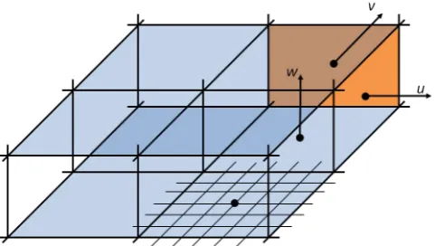
The atmospheric model operates on a logically quadrilat-eral 3-D grid on the Earth surface, and uses a sequence of horizontally nested grids, called domains. Only the inner-most (the finest) atmospheric domain is coupled with the fire model; see also Sect. 8. Scalar variables in the atmospheric model are located at the centers of the 3-D grid cells, while the wind vector components are at a staggered grid at the midpoints of the cell faces. The fire model operates on a refined fire mesh (Fig. 1), and all of its variables are all rep-resented by their values at the centers of the cells of the fire mesh.
3 Fire model
The physical fire model is described in Sects. 3.1, 3.2, and 3.3. It consists of functions specifying the fire spread rate and the heat fluxes, and it is essentially the same as a subset of CAWFE (Clark et al., 2004; Coen, 2005). The spread rate calculation is in turn based on BEHAVE (Rothermel, 1972; Andrews, 2007). It is described here in more detail for the sake of reproducibility and to point out the (minor) differ-ences.
The mathematical core of the fire model is described in Sects. 3.4, 3.5, and 3.6. It consists of the numerical algo-rithms for the fireline propagation, fuel computation, and re-lated functions, such as ignition. The core is independent of any particular fire spread and burn models, and it operates on dimensionless variables. This description here is based on Mandel et al. (2009), with numerous updates and the new developments announced in the introduction.
3.1 Fuel properties
Fuel is characterized by the quantities listed in Table 1, which are given at every point of the fire mesh. To simplify the specification of fuel properties, fuels are given as one of 13 Anderson (1982) categories, which are preset vectors of val-ues of the fuel properties. These valval-ues are specified in an input text file (namelist.fire), and they can be modi-fied by the user. The user can also specify completely new, custom fuel categories.
The fire spread model is based on average values of fuel properties. The fuel categories assign a single vector of fuel coefficients to a fairly broad description of vegetation cover, with similar average fire propagation properties. In prepro-cessing, downscaling and upscaling fuel category data to the fire mesh resolution is handled in WPS by setting a cell in the model to whatever category is dominant in the data for that area.
Fig. 1. One 2×2 tile with the lowest layer of the atmospheric grid and the fire mesh on the surface shown. Wind vector components
u,v,ware located at the midpoints of the sides of the atmospheric grid cells. Some faces are colored for perspective.
3.2 Fire spread rate
The fire model is posed in the horizontal (x, y) plane the Earth surface is projected on. The semi-empirical approach to fire propagation used here assumes that the fire spread rate is given by the modified Rothermel (1972) formula
S=R0(1+φW+φS), (1) whereR0is the spread rate in the absence of wind,φWis the wind factor, andφS is the slope factor. The components of Eq. (1) are computed from the fuel properties (Table 1), the wind speedU, and the terrain slope tanφfollowing the equa-tions in Table 2. The wind speedUis at the so-called mid-flame level, which is one of the quantities given in the fuel categories. We support interpolation to 6.1 m (21 ft) and the use of wind reduction factors (Baughman and Albini, 1980), as well as direct interpolation of the wind to a given mid-flame level; see Sect. 5.2. We refer to Rothermel (1972) for further details, derivation, and justifications of the computa-tion of the terms in Eq. (1). The only differences here from Rothermel (1972) are the subtraction of the moisture from the fuel load in the computation rather than up front, limit-ing the slope and the windspeed, and the explicit reduction of wind to midflame height.
The spread rate can be written as S=max
n
S0,R0+cmin{e,max{0,U}}b+dmax{0,tanφ}2 o
, (2)
whereS0,R0,b,c,d,eare the fuel-dependent coefficients that represent the spread rate internally. These coefficients are stored for every grid point. The representation of the spread rate by Eq. (2) supports also other models, such as a chaparral model from Clark et al. (2004).
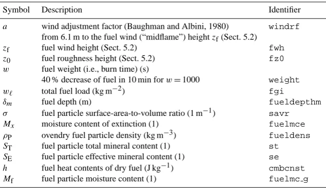
Table 1. Fuel properties. The notation is from Rothermel (1972) except as indicated. The identifiers are as used in SFIRE or CAWFE. In the input files, some quantities are given in English units per Rothermel (1972); see Wang et al. (2010, p. A-5).
Symbol Description Identifier
a wind adjustment factor (Baughman and Albini, 1980) windrf from 6.1 m to the fuel wind (“midflame”) heightzf(Sect. 5.2)
zf fuel wind height (Sect. 5.2) fwh
z0 fuel roughness height (Sect. 5.2) fz0
w fuel weight (i.e., burn time) (s)
40 % decrease of fuel in 10 min forw=1000 weight
w` total fuel load (kg m−2) fgi
δm fuel depth (m) fueldepthm
σ fuel particle surface-area-to-volume ratio (1 m−1) savr
Mx moisture content of extinction (1) fuelmce
ρP ovendry fuel particle density (kg m−3) fueldens
ST fuel particle total mineral content (1) st
SE fuel particle effective mineral content (1) se
h fuel heat contents of dry fuel (J kg−1) cmbcnst
Mf fuel particle moisture content (1) fuelmc g
normal component of the terrain gradient, tanφ= ∇z·n, are used to determine the spread rate, which is interpreted as the spread rate in the normal directionn.
3.3 Fuel burned and heat released
Each location starts with fuel fractionF=1. Once the fuel is ignited at a timeti, the fuel fraction decreases exponentially,
F (t )=exp
−(t−ti)
Tf
, t > ti, (3) wheret is the time, ti is the ignition time,F0 is the initial amount of fuel, andTfis the fuel burn time, i.e., the number of seconds for the fuel to burn down to 1/e≈0.3689 of the original quantity. Since by definition of the fuel weightw (Table 1), the fuel burns down to 0.6 of the original quantity in 600 s whenw=1000, we have
0.6(t −ti) 600
1000 w =exp
−(t−ti)
Tf
,
which gives Tf= −
600w 1000ln0.6≈
w 0.8514.
The input coefficientwis used in SFIRE rather thanTf for compatibility with existing fuel models and literature. The fuel weightwis given by the user in the input data as one of the coefficients in the fuel categories. The default values are from the CAWFE code, which, according to Clark et al. (2004, p. 55), were chosen to approximate the mass-loss curve from the BURNUP algorithm (Albini and Reinhardt, 1995). The speed of burning is currently taken to be indepen-dent of the wind speed and the fuel moisture. Taking these
factors into consideration is a subject of future research, and it will have to be justified by comparison with experiments.
The average sensible heat flux density released in time in-terval(t,t+1t )is computed as
φh=
F (t )−F (t+1t ) 1t
1 1+Mf
w`h,
W m−2 (4)
and the average latent heat (i.e., moisture) flux density is given by
φq=
F (t )−F (t+1t ) 1t
Mf+0.56
1+Mf
Lw`,
W m−2 (5) where 0.56 is the estimated mass ratio of the water output from the combustion to the dry fuel, andL=2.5×10⁶J kg−1 is the specific latent heat of condensation of water at 0◦C,
used for nominal conversion of moisture to heat. This com-putation is from CAWFE.
It should be noted that there is significant uncertainty in the data as well as in the approximations made above, and many factors that influence the spread rate are not accounted for. See Sect. 10.3 for a more complete discussion and possible future improvements.
3.4 Fire propagation by the level set method
The model maintains a level set functionψ, the time of igni-tionti, and the fuel fractionF. Denote a point on the surface byx=(x,y). The burning region at timetis represented by a level set functionψ=ψ (x,t )as the set of all pointsxsuch that ψ (x,t )≤0. There is no fire at x if ψ (x,t ) >0. The fireline is the set of all pointsxsuch thatψ (x,t )=0. On the fireline, the tangential component of the gradient∇ψis zero. Hence, the outside normal vector at the fireline is
n= ∇ψ
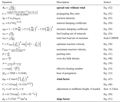
Table 2. Computation of the fire spread rate factors in (1) from the fuel properties (Table 1), the wind speedUat 6.1 m, and the terrain slope tanφ. All equations are from Rothermel (1972) unless otherwise indicated. All input quantities are first converted from metric to English units (BTU-lb-ft-min) to avoid changing the numerous constants in the Rothermel (1972) computations. Further, following CAWFE, the wind is limited to between 0 and 30 m s−1and the slope is limited to nonnegative values. The values marked in bold are the final factors that enter into the spread rate computation (1).
Equation Description Source
R0= IRξ
ρbεQig spread rate without wind Eq. (52)
ξ=exp
0.792+0.681σ0.5
(β+0.1)
192+0.2595σ propagating flux ratio Eq. (42)
IR=0wnhηMηs reaction intensity Eq. (52)
ηs=0.174Se−0.19 mineral damping coefficient Eq. (30)
ηM=1−2.59MfMx+5.11
Mf
Mx 2
−3.52MfMx3 moisture damping coefficient Eq. (29)
wn= w0
1+ST fuel loading net of minerals Eq. (24)
w0=1+wMf` total fuel load net of moisture from CAWFE
0=0max
β βop
A
exp
h
A
1− β
βop i
optimum reaction velocity Eq. (36)
0max= σ1.5
495+0.594σ1.5 maximum reaction velocity, Eq. (36)
β=ρb
ρP packing ratio Eq. (31)
ρb=wδ0 oven dry bulk density Eq. (40)
A= 1
4.77σ0.1−7.27 Eq. (39)
ε=exp
−138
σ
effective heating number Eq. (14)
Qig=250β+1116Mf heat of preignition Eq. (12)
φW=CmaxUaβ
β
βop E
wind factor Eq. (47)
C=7.47exp−0.133σ0.55 Eq. (48)
Ua=aUorUa=U adjustment to midflame height, if needed Sect. 5.2 here
E=0.715exp−3.59×10⁻⁴σ Eq. (50)
φS=5.275β−0.3tan2φ slope factor Eq. (51)
Now consider a pointx(t )that moves with the fireline. Then the fire spread rateSatxin the direction of the normal nis
S=n·∂x
∂t, (7)
and, from the definition of the fireline,ψ (x(t ),t )=0. By the chain rule and substituting from Eqs. (6) and (7), we have 0= d
dtψ (x,t )= ∂ψ
∂t + ∂ψ
∂x ∂x ∂t +
∂ψ ∂y
∂y ∂t
= ∂ψ
∂t + k∇ψk
n·∂x
∂t
=∂ψ
∂t +Sk∇ψk. (8) So, the evolution of the level set function is governed by the partial differential equation
∂ψ
∂t +Sk∇ψk =0, (9)
called the level set equation (Osher and Fedkiw, 2003). The spread rateS is evaluated from (2) for allx, not just on the fireline. SinceS≥0, the level set function does not increase with time, and the fire area cannot decrease, which also helps with numerical stability by eliminating oscillations of the level set functionψin time.
To advance the fire region in time, we use Heun’s method (Runge-Kutta method of order 2),
ψn+1/2=ψn+1t F ψn
ψn+1=ψn+1t
1
2F ψ
n
+1
2F
ψn+1/2
, (10) The right-hand side F is a discretization of the term
−Sk∇ψkwith upwinding and artificial viscosity, F (ψ )= −S (U·n,∇z·n)
∇ψ
+ε4eψ, (11)
wheren= ∇ψ/k∇ψkis computed by finite central differ-ences and∇ψ=∇xψ,∇yψis the upwinded finite differ-ence approximation of∇ψby the essentially nonoscillatory (ENO) method of order one (Osher and Fedkiw, 2003, p. 59),
∇xψ=
∇+xψ if∇−xψ≤0 and∇+xψ≤0,
∇−xψ if∇−xψ≥0 and∇+xψ≥0,
∇−xψ if∇−xψ≥0 and∇+xψ≤0,and
∇ − xψ ≥ ∇ + xψ ,
∇+xψ if∇−xψ≥0 and∇+xψ≤0,and
∇ − xψ < ∇ + xψ ,
otherwise 0,
(12)
where∇x+ψand∇x−ψare the right and left one-sided finite differences
∇x+ψ (x,y)= ψ (x+ 4x,y)−ψ (x,y) 4x ,
∇x−ψ (x,y)= ψ (x,y)−ψ (x− 4x,y) 4x ,
and similarly for∇y+ψand∇y−ψ. Further, in Eq. (11),εis scale-free artificial viscosity (ε=0.4 here), and
e
4ψ = ∇+
xψ− ∇ − xψ+ ∇
+ yψ− ∇
− yψ
=ψ (x+ 4x,y)−2ψ (x,y)+ψ (x− 4x,y) 4x
+ similar term for y
is the five-point Laplacian ofψ scaled so that the artificial viscosity is proportional to the mesh step,
e
4ψ≈ 4x∂ 2ψ ∂x2 + 4y
∂2ψ ∂y2.
Although the ENO method theoretically should alone be suf-ficient to prevent instabilities, we have found that the addi-tional viscosity was needed, otherwise in some cases insta-bilities do occur.
A numerically stable scheme with upwinding, such as Eq. (12), is required to compute the termk∇ψkin the level set Eq. (9). However, in our tests, the gradient by standard central differences,
∇ψ≈
ψ (x+ 4x,y)−ψ (x− 4x,y)
24x ,
ψ (x,y+ 4y)−ψ (x,y− 4y) 24y
,
worked better in the computation of the normal vectornby Eq. (6), which is used to evaluate the normal component of the wind and the slope in Eq. (2).
We have found that even if the scheme is first-order in space, a second-order method in time was required. For a first-order method (Euler’s method), there was too much sys-tematic error in the positive direction, causing the fire to dis-appear quickly.
Before computing the finite differences up to the bound-ary, the level set function is extrapolated to one layer of nodes beyond the boundary. However, the extrapolation is not al-lowed to decrease the value of the level set function to less than the value at either of the points it is extrapolated from. For example, when(i,j )is the last node in the domain in the directionx, the extrapolation
ψi+1,j=maxψij+ ψij−ψi−1,j,ψij,ψi−1,j ,
is used, and similarly in the other cases. This is needed to avoid numerical instabilities at the boundary. Otherwise, a decrease inψ at a boundary node, which may happen with non-homogeneous fuels in real data, is amplified by the ex-trapolation, andψkeeps decreasing at that boundary node in every time step until it becomes negative, starting a spurious fire.
The model does not support fire crossing the boundary of the domain. Whenψ <0 is detected near the boundary, the simulation terminates. This is not a limitation in practice, because the fire should be well inside the domain anyway for a proper response of the atmosphere.
The ignition time ti in the strip that the fire has moved over in one time step is computed by linear interpolation from the level set function. Suppose that the point x is not burning at timet but is burning at timet+ 4t, that is, ψ (x,t ) >0 andψ (x,t+ 4t )≤0. The ignition time atx sat-isfiesψ (x,ti(x))=0. Approximatingψby a linear function in time, we have
ψ (x,ti)−ψ (x,t ) ti(x)−t
≈ψ (x,t+ 4t )−ψ (x,ti)
t+ 4t−ti(x) ,
and we take ti(x)=t+
ψ (x,t )4t
ψ (x,t )−ψ (x,t+ 4t ). (13) 3.5 Computation of the fuel fraction
The fuel fraction is approximated over each fire mesh cellC by integrating Eq. (3) over the fire region. Hence, the fuel fraction remaining in cellCat timetis given by
F=1− 1
area(C)
ZZ
x∈C ψ (x,t )≤0
1−exp
−t−ti(x)
Tf(x)
dx. (14)
that the total heat released in the atmosphere over time is ex-act, regardless of approximations in the computation of the integral Eq. (14). Our objective in the numerical evaluation of Eq. (14) is a method that is second order accurate when the whole cell is on fire, exact when no part of the cellC is on fire (namely, returning the value one), and provides a natural transition between these two cases. Just like stan-dard schemes in numerical analysis can be derived from the requirement that they are exact for all polynomials up to a given degree, the guiding principle here is that the scheme should be exact in as many special cases as possible. Then we expect that the scheme should work well overall.
While the fuel burn timeTfcan be interpolated as constant over the whole cell, the level set functionψand the ignition timetimust be interpolated more accurately to allow a sub-mesh representation of the burning area and a gradual release of the heat as the fireline moves over the cell. In addition, we need the fuel fraction computed over each mesh cell, because the heat fluxes in the mesh cells are summed up to give the heat flux in an atmospheric cell. Our solution is to split each cell into 4 subcellsCj, interpolate to the corners of the
sub-cells, and add the integrals,
ZZ
x∈C ψ (x)≤0
1−exp
−t−ti(x)
Tf(x)
dx
=
4
X
j=1
ZZ
x∈Cj
ψ (x)≤0
1−exp
−t−ti(x)
Tf(x)
dx, (15)
cf., Fig. 2. The level set functionψis interpolated bilinearly to the vertices of the subcellsCj, and the burn time Tf is constant on eachCj, given by its value at the fire grid nodes.
When the whole cellCis on fire (that is,ψ≤0 on all four vertices ofC),tiis interpolated also linearly to the vertices of the subcellsCj. However, the case when the fireline crosses
the cellC requires a special treatment of the ignition time ti; ti(x)has meaningful value only when the nodex is on fire,ψ (x)≤0. Also, on the fireline,ψ (x)=0 andti(x)=t. Thus, approximating bothψandtiin the fire region by linear functions suggests interpolating from the relation
ti−t=cψ, (16)
for somec. We interpolate on the grid lines between two nodes first. If both nodes are on fire, we interpolate ti bilinearly as before. However, when one cell center is on fire and one not, say ψ (a1) >0, ψ (a2) <0, we find the proportionality constantcin Eq. (16) fromti(a2)=cψ (a2), and setti(b)=cψ (b)at the midpointb=(a1+a2)/2. In the case of interpolation to the node c=(a1+a2+a3+a4)/4 between nodes a1,a2,a3,a4, we find the proportionality constantcby solving the least squares problem
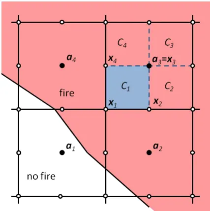
Fig. 2. Division of fire mesh cells into subcells for fuel fraction computation. The level set functionψ and the ignition timetiare
given at the centersa1,...,a4of the cells of the fire grid. The in-tegral (15) over the cellC with the centera3is computed as the
sum of integrals over the subcellsC1,...,C4. While the values of ψ andtiare known ata3=x3, they need to be interpolated to the
remaining cornersx1,x2,x4of the subcellC1from their values at the pointsa1,...,a4.
4
X
j=1
ψ(aj)≤0
ti aj−t−cψ aj
2
→min
and set againti(c)=cψ (c).
To compute the integral over a subcellCj, we first estimate
the fraction of the subcell that is burning, by
areax∈Cj:ψ (x)≤0 area(Cj)
≈β=1
2 1−
P4
k=1ψ (xk)
P4
k=1|ψ (xk)|
!
, (17) wherexkare the the corners of the subcellCj. This
approxi-mation is exact when no part of the subcellCj, is on fire, that
is, allψ (xk)≥0 and at least oneψ (xk) >0; the wholeCj
is on fire, that is, allψ (xk)≤0 and at least oneψ (xk) <0;
or the valuesψ (xk)define a linear function and the fireline
crosses the subcell diagonally or it is aligned with one of the coordinate directions.
Next, replaceti(xk)byt whenψ (xk) >0 (i.e., the node
xk is not on fire), and compute the approximate fraction of
the fuel burned as 1
area(C)
ZZ
x∈C ψ (x,t )≤0
1−exp
−t−ti(x)
Tf(x)
dx
≈β 1−exp −1
4 4
X
k=1
ti(xk)−t
Tf
!!
This calculation is accurate asymptotically when the fuel burns slowly and the approximationβ of the burning area is exact.
3.6 Ignition
Typically, a fire starts from a horizontal extent much smaller than the fire mesh cell size, and both point and line igni-tion need to be supported. The previous igniigni-tion mechanism (Mandel et al., 2009) ignited everything within a given dis-tance from the ignition line at once. This disdis-tance was re-quired to be at least one or two mesh steps, so that the initial fire is visible on the fire mesh, and the fire propagation algo-rithm from Sect. 3.4 can catch on. This caused an unrealisti-cally large initial heat flux and the fire started too fast.
The current ignition scheme achieves submesh resolution and zero-size ignition. A small initial fire is superimposed on the regular propagation mechanism, which then takes over. Drip-torch ignition is implemented as a collection of short ignition segments that grows at one end every time step. Mul-tiple ignition segments are also supported.
The model is initialized with no fire by choosing the level set functionψ (x,t0)=const>0. Consider an initial fire that starts at timetg on a segmenta,band propagates in all di-rections with an initial spread rateSguntil the distancergis reached. At the beginning of every time steptsuch that tg≤t≤tg+
rg Sg ,
we construct the level set function of the initial fire, ψg(x,t )=dist
x,a,b−Sg t−tg (19) and replace the level set function of the model by
ψ (x,t ):=min
ψ (x,t ),ψg(x,t ) . (20) For a drip-torch ignition starting from pointaat timetgat ve-locityvuntil timeth, the ignition line at timetis the segment a,a+v min{t,th} −tg, and Eq. (19) becomes
ψg(x,t )=dist
x,a,a+v min{t,th} −tg
−minrg,Sg t−tg
followed again by Eq. (20), at the beginning of every time step begining at timetsuch that
tg≤t≤th+ rg Sg .
The ignition time of newly ignited nodes is set to the arrival time of the fire at the spread rateSgfrom the nearest point on the ignition segment.
4 Atmospheric model
We summarize some background information about WRF-ARW from Skamarock et al. (2008), to the extent needed to understand the coupling with the fire module.
The model is formulated in terms of the hydrostatic pres-sure vertical coordinateη, scaled and shifted so thatη=1 at the Earth surface andη=0 at the top of the domain. The governing equations are a system of partial differential equa-tions of the form
d8
dt =R (8), (21)
where R contains also the advection terms, and 8=
U,V ,W,φ0,2,µ0,Qm. The fundamental WRF variables areµ=µ(x,y), the hydrostatic component of the pressure differential of dry air between the surface and the top of the domain, written in perturbation formµ=µ+µ0, whereµ is a reference value in hydrostatic balance;U=µu, where u=u(x,y,η)is the Cartesian component of the wind veloc-ity in thex-direction, and similarlyV andW;2=µθ, where θ=θ (x,y,η) is the potential temperature;φ=φ (x,y,η)=
φ+φ0 is the geopotential; andQm=µqm is the moisture content of the air. The variables in the state8evolved by Eq. (21) are called prognostic variables. Other variables computed from them, such as the hydrostatic pressurep, the thermodynamic temperatureT, and the heightz, are called diagnostic variables. The variables that containµare called coupled. The value of the right-hand sideR (8)is called ten-dency. See Skamarock et al. (2008, p. 7–13) for details and the form ofR.
The system (21) is discretized in time by the explicit 3rd order Runge-Kutta method
81=8t+ 1t
3 R 8
t
82=8t+ 1t
2 R (81)
8t+1t =8t+1t R (82) (22) where the differential operatorR is discretized by finite dif-ferences and the tendencies from physics packages, such as the fire module, are updated only the third Runge-Kutta step (Skamarock et al., 2008, p. 16). In order to avoid small time steps, the tendency in the third Runge-Kutta step also includes the effect of substeps to integrate acoustic modes.
5 Coupling of the fire and the atmospheric models 5.1 Interpolation of the terrain gradient
jumps in the gradient, unless high-order interpolation is used, which cause unnatural fire propagation with the fire changing direction at the location of the jumps of the gradient. 5.2 Wind interpolation and wind reduction factors Wind is interpolated horizontally from the atmospheric mesh to the fire mesh, and vertically to a given “midflame” height zfabove the terrain (Baughman and Albini, 1980) by assum-ing the ideal logarithmic wind profile
u(z)≈
clnz
z0, z≥z0,
0 0≤z≤z0,
(23) wherezis the height above the terrain,z0is the roughness height, andcis a proportionality constant.
The vertical interpolation algorithm is as follows. For a given horizontal location, denote byz1,z2,...the heights of the atmospheric grid mid-levels and byu(z1),u(z2),...the values of theuhorizontal wind component at those heights. The heightszk are computed from the geopotentialφ, which
is a part of the solution in WRF. The horizontal wind com-ponents u at zk are then found by horizontal interpolation
from the atmospheric mesh, and interpolated vertically to the given heightzfby log-linear interpolation. That is,u(zf)is determined by 1-D piecewise linear interpolation of the val-uesu(z0)=0,u(z1),u(z2),...at lnz0, lnz1, lnz2,...to lnzf; ifzf≤z0, we set u(zf)=0. Thev component of the wind is interpolated in the same way. The computation is orga-nized in such way that only the vertical levels that are actu-ally needed are evaluated above every fire mesh node.
Note that the vertical interpolation is exact if the wind pro-file obeys the logarithmic propro-file Eq. (23) exactly. This is a desirable property in numerical analysis: for example, linear interpolation can be defined by the fact that it is exact for all linear functions.
A commonly used value for the roughness height isz0= 0.13H, whereH is the height of the vegetation. The rough-ness heightz0and the heightzfto interpolate to (the “mid-flame” height) are properties of the fuel category, and they are given by the user in input data. The roughness height is also known from land use in WRF, though that value may not be the same.
We also support the use of the wind reduction factors, fol-lowing Baughman and Albini (1980). The wind reduction (or adjustment) factora is used to determine the vertically interpolated windu(zf)from wind measured at a reference height zref (20ft=6.096m in BEHAVE), by assuming the ideal logarithmic wind profile (23):
u(zf)=au(rref). (24)
From (23) withz=zfandz=zref, we have u(zf)=cln
zf z0 ,
u(zref)=cln zref
z0 ,
which gives the wind reduction factora from the roughness heightz0and the interpolation heightzfas
a= ln
zf z0
lnzref z0
. (25)
The wind reduction factors for the 13 fuel categories are available in Baughman and Albini (1980, Table 3, p. 91). Equation (25) then allows to find the interpolation heights from the reduction factors as
zf=(zref)a(z0)1−a. (26) In summary, we suggest two options for the vertical inter-polation:
1. Interpolate to the fire mesh and then to the heightzfas described at the beginning of this section, and do not re-duce the wind by the adjustment factora. This option is preferable whenz1< zref, because otherwise some in-formation is lost, and it may be used in any case. 2. Interpolate vertically to the common height zref, then
horizontally to the fire mesh, and use the wind reduction factorsa given at the points of the fire mesh, following Eq. (24). This option is much simpler and cheaper, but it may lose information on the actual wind profile under the heightzref.
Both options are mathematically equivalent when the verti-cal resolution is so coarse thatz1≥zref, as is usually the case except in microscale computations. Either option can be se-lected when running the code.
5.3 Time step
In each time step of the atmospheric model, the fire mod-ule is called from the third step (22) of the Runge-Kutta method in WRF-ARW. First, the wind is interpolated follow-ing Sect. 5.2 for use in the spread rate formula Eq. (1). The fire model then makes its own time step:
1. If there are any active ignitions, the level set function is updated and the ignition times of any newly ignited nodes are set following Sect. 3.6.
2. The numerical scheme (10–12) for the level set Eq. (9) is advanced to the next time step.
3. The time of ignition set for any any nodes that were ignited during the time step, from Eq. (13).
4. The fuel fraction is updated following Sect. 3.5. 5. The sensible and latent heat flux densities are computed
6. The resulting heat flux densities are averaged over the fire cells that make up one atmosphere model cell, and inserted into the atmospheric model, as described in the next Sect. 5.4.
The atmospheric model then completes the time step. 5.4 Inserting fire heat fluxes into the atmosphere The heat fluxes from the fire are inserted into the atmo-spheric model as forcing terms in the differential equations of the atmospheric model into a layer above the surface, with assumed exponential decay with altitude. Such scheme is needed because WRF does not support flux boundary condi-tions. This is code originally due to Clark et al. (1996a,b) and it was rewritten for WRF variables in Patton and Coen (2004). The sensible heat flux is inserted as an additional source term to the equation for the potential temperatureθ, equal to the vertical divergence of the heat flux,
d (µθ )
dt (x,y,z)=R2(8)+
µ(x,y)φh(x,y) σ %(x,y,z)
∂ ∂zexp
− z zext
,
whereR2(8) is the component of the source term
(com-monly called “tendency” in the WRF code) in the at-mospheric model Eq. (21), σ is the specific heat of the air, %(x,y,z) is the density, and zext is the heat ex-tinction depth, given as parameter fire ext grnd in
namelist.input. The latent heat flux is inserted simi-larly into the source term of the vapor concentrationqmby d (µqm)
dt (x,y,z)=RQm(8)+
µ(x,y)φq(x,y) L%(x,y,z)
∂ ∂zexp
− z zext
,
whereLis the specific latent heat of the air. Cf. Clark et al. (1996a, Eqs. 10, 12, 13, 18).
6 Parallel structure and limitations
Parallel computing is essential for fast execution, yet it im-poses a significant constraint on user programming tech-nique. At the danger of some simplification, one can say that WRF parallel infrastructure (Michalakes, 2000) essen-tially divides the domain horizontally into rectangular re-gions, called tiles, and different tiles are assigned to differ-ent processor cores, which execute in parallel. A numerical code in WRF needs to be tile callable. This means that the code runs on a single tile, using values from strips around the tile boundary in neighboring tiles, if necessary. The val-ues in those strips may not be changed while the tile-callable code executes, and they are communicated by other code only after the tile-callable code exists. The communication in fact happens in two different ways, called MPI and OpenMP (Fig. 3), corresponding to distributed memory scheme (es-sentially, separate computers connected by a network) and shared memory (multiple processor cores in a single com-puter).
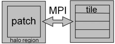
Fig. 3. Parallel communication in WRF. The computational domain is divided into disjoint rectangular patches. Each patch is updated by a single MPI process (distributed memory parallelism), and the process may read arary data in a strip around the patch, called halo region. The communication between the patches is by halo calls to the RSL parallel infrastructure (Michalakes, 2000), which update the halo regions by the values from the neighboring patches. Each patch may be divided into tiles, which execute in separate OpenMP threads (shared memory parallelism). Following WRF coding con-ventions (WRF Working Group 2, 2007), computational kernels ex-ecute in a single tile. They may read array values from a strip be-yond the tile boundary but no explicit communication is allowed. 3-D arrays are divided into patches and tiles in the horizontal plane, cf., Fig. 1.
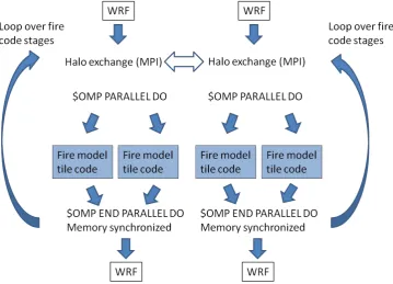
Consequently, numerical code must execute in stages, al-ternating between numerical computing and communicating values between the strips (Fig. 4), while going down the soft-ware layers (Fig. 5) in each stage to resume the computation. The fire module code executes in 6 stages interleaved with communication, 3 stages for initialization and 3 stages in ev-ery time step. For small tiles, the communication dominates the computational cost, which puts a practical limit on the number of processor cores that may be used for any given problem.
Unfortunately, the parallel computing structure limits the class of numerical methods that are feasible to implement. In particular, high-order methods, which need to update values at a node using values from distant nodes are no longer very practical, both because of the complexity of programming and because of the sharply increased communication cost. This explains our choice of numerical methods of the lowest possible order.
7 Data input
WRF and SFIRE may be run in both “ideal” and “real” modes, which require slightly different setups. Ideal runs were extended by adding fire-related capabilities, such as reading fuel, topography, and land use from simple text files. This allows to run simulations which go beyond what would normally be considered an ideal run and simplifies custom data input; the simulation of the FireFlux experiment (Sect. 9) was done in this way.
Fig. 4. Parallel structure of the fire module in the WRF physics layer. The core code itself executes on a single tile, with all communication done outside. Multiple passes through the fire module are needed in each time step.
the WRF Preprocessing System (WPS) (Wang et al., 2010, Chapter 3), which contains a number of utilities useful for preparing standard atmospheric and surface datasets for in-put into WRF. In a real run, a user must supply data for the initial and boundary conditions for the WRF simulation.
WPS has been extended (Beezley, 2011) with the abil-ity to produce data defined on the refined surface meshes used by SFIRE (Sect. 8); however, it is not possible to dis-tribute high resolution, global fields as is done in the stan-dard dataset. Instead, the user must download any neces-sary high resolution fields and convert them for each sim-ulation. The WPS extensions include the ability to input data in GeoTIFF format, which is a standard file format for high-resolution geoscientific data, such as aerial and satel-lite images. See http://www.openwfm.org/wiki/How to run WRF-Fire with real data for details.
For a SFIRE simulation, it is only strictly necessary to download one additional dataset. This dataset contains the map of fuel categories on the simulation domain.. For simu-lations within the United States, this data can be obtained in GeoTIFF format from the USGS at http://www.landfire.gov. SFIRE uses an additional variable for high-resolution topog-raphy, which is allowed to be different from the topography used used by the atmospheric code. This is useful because a high resolution WRF simulation generally requires the to-pography to be highly smoothed in preprocessing for numer-ical stability. The fire code can benefit from a rougher topog-raphy for more accurate fire spread computations.
For atmospheric data, it is best to use the highest resolution dataset available to initialize a WRF simulation to capture as much of the local conditions near the fire as possible. Gener-ally, publicly available atmospheric data is limited to around 10 km resolution. As a consequence, one should create sev-eral nested grids, each with a 3 to 1 refinement ratio, and a long spin-up prior to ignition in order to recreate local con-ditions. Preliminary results indicate that assimilation of data from weather stations or satellite radiances may be required for an accurate simulation (Beezley et al., 2010).
8 WRF settings
Since the coupled code initialization for the real cases does not differ from the one for the regular WRF, all physical and dynamical options available in the regular WRF are also available. Therefore, the same general rules apply to the con-figuration as to the concon-figuration of the regular WRF. 8.1 Domains and nesting
However, one should keep in mind that resolutions of the finest domains in fire simulations are usually significantly higher than in weather forecasting applications. This has two consequences in terms of the proper WRF setup for SFIRE. First, if the resolution of any of the inner domains is less than
100 m, this domain should be actually resolved in the large eddy simulation (LES) mode, without the boundary layer pa-rameterizations. At this resolution, the model should be able to resolve the most energetic eddies responsible for mixing within the boundary layer, so the boundary layer parame-terization in this case is not needed. Second, since in the nested mode, vertical levels are common for all domains, the height of the first model level selected for the most outer (par-ent) domain, defines also the level of the first model layer for all inner (child) domains, even if their horizontal reso-lutions are an order of magnitude smaller. The fact that the vertical model resolution is the same for all domains signif-icantly limits the minimum height above the ground of the first model level. This in turn is crucial for the fire model, which uses the wind speed interpolated to 6.1 m or less above the ground. Therefore, in the cases when the first model level must be relatively high above the ground it is recommended to perform only one way nesting, which allows the use of different vertical levels on different domains.
8.2 Large Eddy Simulation and surface properties To enable the high-resolution simulation in Large Eddy Sim-ulation (LES) mode, user should first disable the boundary layer parameterization (bl pbl physics=0). The LES mode requires the proper surface fluxes in order work prop-erly. We recommend the optionisfflx=1, which makes WRF use a surface model to compute the surface fluxes. Other options with constant heat fluxes and drag are not well suited for fire simulations. Out of all surface exchange parameterizations only the classic Monin-Obukhov theory (sf sfclay physics=1) is recommended for the LES cases. This option assures a proper computation of face transfer coefficients that are used together with the sur-face properties (provided by the sursur-face model) for com-putation of the surface fluxes of the momentum, heat and moisture. The surface model itself computes properties of the surface, but does not compute the surface exchange co-efficients, which are needed for computation of the surface fluxes. Hence, in order to compute them, the surface proper-ties must be provided by a surface model, which is enabled by choosing a non-zerosf surface physics. The sub-grid scale parameterization used by the WRF in LES mode is defined by thekm optparameter, which should be set to 2 (TKE closure), or 1 (Smagorinsky scheme).
In real cases, proper initialization for the selected land sur-face model is provided automatically, and all other compo-nents. In ideal cases, users are responsible for the proper initialization and setting land use properties.
8.3 Mesh resolution and refinement ratios
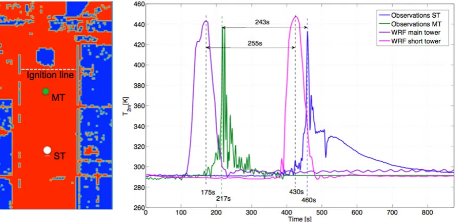
Fig. 6. Simulation of the FireFlux experiment (Clements et al., 2007) by WRF and SFIRE. Left: map of landuse category for the experimental plot, with the ignition line and the observation towers marked. Right: simulated and measured temperature profiles at the location of the observation towers. The simulated fire propagation takes 243 s from tower MT to tower ST, while the measured time is 255 s (4.7 % difference). Due to the instrument failure that took place during the experiment about 20 s after the fire front passage, the recorded temperature drop is unrealistically slow, and do not represent the actual cooling phase. Therefore, the discrepancies in the temperature drop at the short tower should not be treated as an indication of the model error. The turbulent kinetic energy and the wind profile at that tower were captured well and they do not indicate specific problems associated with realistic rendering of the post fire cooling. From Kochanski et al. (2010).
at such fine resolution. The atmospheric mesh step should be about 60 m or less for proper feedback of the wind on the fire line. Larger mesh step was reported to result in too large fire spread rates in interaction with the atmosphere (Clark et al., 1996a, p. 887); however, we did not observe this.
Because of the computational cost, the practical limit of the atmospheric domain resolution for forecasting applica-tions seems to be currently around 400 m. At that resolution, the simulation to wall clock time ratio may be kept around 6, that is, 24 h forecast may be completed within 4h. The limiting factor is the short time step required for higher res-olutions. Using more processor cores (Sect. 6) for a fixed problem eventually reaches the point of diminishing return, because each core gets a smaller domain to work on and the parallel efficiency decreases. One should keep in mind that even this relatively coarse atmospheric resolution (from the fire modeling point of view) already extends beyond the max-imum resolution of the standard meteorological static surface data, which is currently 1 km. At the atmospheric model res-olution of 400 m, the refinement ratio of 10 brings the fire model mesh size close to maximum resolution of the avail-able fuel data, which is currently 30 m. So, from the fuel data point of view, running real forecasting simulations at higher than 30 m resolutions does not seem practical. How-ever, since the fire spread depends on the slope gradient that is computed on the fire mesh, using finer fire model mesh in
complex terrain may be justified. The topographical data are generally available at higher resolutions than the fuel maps (for the US, it is 2 m), so in cases when the sub-grid variabil-ity in the fuel composition is expected to be relatively small, and the topographical effects are expected to be important, further increasing of the fuel model resolution beyond the 30 m limit may be desirable.
From the point of view of the atmosphere-fire interac-tion, a coarser horizontal and vertical atmospheric resolu-tion means less intense feedback from fires of the burning area smaller than the atmospheric grid cells, since the fire heat flux computed on the fire mesh gets averaged over a bigger atmospheric cell. Smaller heat flux leads to weaker fire-induced updraft, less intense surface convergence and fi-nally weaker wind speed up at the fire front, which in turn could theoretically result in underestimation of the fire rate of spread. However, since the Rothermel fire model was cal-ibrated, based on undisturbed wind speed measured upwind from the fireline at 6.1 m height, the local speed up at the fire line has been already captured by the model constants. Whether further adjustments to the fire parameterization are needed, depending on the resolution and fiatmosphere re-finement ratio, is a question for future research.
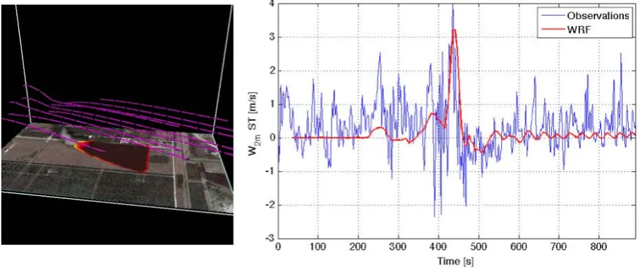
Fig. 7. Simulation of the FireFlux experiment (Clements et al., 2007) by WRF and SFIRE. Left: surface heat flux and selected flowlines. Visualization in VAPOR by Bedˇrich Soused´ık. Surface image from Google Earth. Right: vertical velocity at 2 m height at tower ST. (See Fig. 6 left for location.) The simulation shows a good agreement with the experiment. From Kochanski et al. (2010).
on the atmosphere-fire coupling with well-known fuel con-ditions, such as the FireFlux experiment (Figs. 6 and 7 ), re-alistic rendering of the atmospheric response to the surface heating associated with fire is absolutely crucial. For these applications, the fire model should use the wind speed taken from the level as close to the mid-flame height as possible. This requirement translates into a need for very high verti-cal resolution. For realistic modeling of the fire of expected flame height of let us say 4 m, the first atmospheric model level should be at 2 m. Updrafts associated with fire plumes may easily reach a rising speed of 5 m s−1, so in order to keep the simulation numerically stable, the time step should not be greater than 0.4 s. Assuming the horizontal wind speeds be-low 25 m s−1, the vertical model resolution will be a limiting factor in terms of the time step as long as the horizontal grid spacing will be greater than 10 m. This reasoning was ap-plied during the design of the FireFlux simulation, for which the horizontal resolution has been set to 10 m, as an optimal value providing high horizontal resolution yet not requiring further reduction in the time step. Detailed analysis of the FireFlux experiment is in progress and will be published as a separate case study elsewhere.
Since the fine-resolution simulations are mostly run in the LES mode as opposed to the coarser real cases that rely on boundary layer parameterization, the degree to which the ver-tical mixing is captured by the model directly depends on the model resolution. From that point of view, the grid refine-ment for fine-resolution cases should be expected to bring more benefits than for real cases utilizing boundary layer and cloud parameterizations, which were originally designed for much coarser atmospheric meshes.
8.4 Time step
In real SFIRE simulations performed in multi-domain con-figurations the time step requirements for the outer domains (run without fire) do not differ from general meteorological cases. The recommended time step of 6 times the horizontal grid spacing (in km) may be used as a starting point. How-ever, for the finest domains run with fire simulations, the time step in most cases must be significantly smaller. For domains with low vertical resolution and simple topography, the hor-izontal mesh step is crucial for numerical stability, since the horizontal velocity is greater than the vertical one. In fire simulations with high vertical resolution, the vertical velocity induced by fire may violate the CFL condition. Therefore, it is advisable to use a vertically stretched grid, with finer res-olution at the surface (where updraft velocities are not that high) and lower resolution at higher levels where stronger updrafts are expected. This allows for having the first model level relatively close to the ground, yet with vertical spacing aloft big enough to handle strong convective updrafts without violating the CFL condition.
9 Computational simulations
9.1 Examples of output and computational results Kim (2011) has verified that the level set method in the fire module advects the fire shape correctly, on some of the same examples that were used to verify the tracer code in CAWFE (Clark et al., 2004).
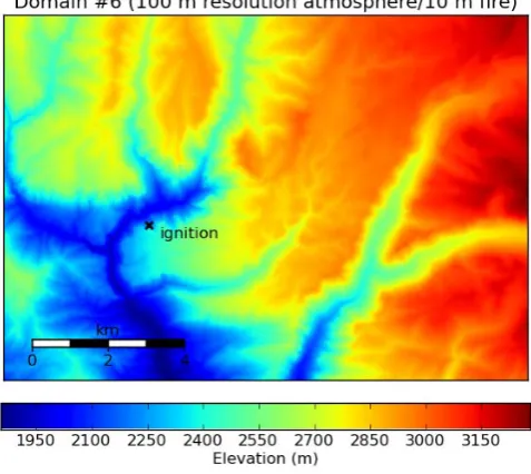
A number of successful simulations with SFIRE now ex-ist. Jenkins et al. (2010) have demonstrated fireline finger-ing behavior for a sufficiently long fireline (Figs. 8 and 9) on an ideal example, with similar results as in Clark et al. (1996a,b). Kochanski et al. (2010) have demonstrated the va-lidity of SFIRE on a simulation of the Clements et al. (2007) FireFlux grass fire experiment and obtained good agreement with data (Figs. 6 and 7). Dobrinkova et al. (2011) simu-lated a fire in Bulgarian mountains using real meteorological and geographical data, and ideal fuel data. Beezley et al. (2010) simulated the 2010 Meadow Creek fire in Colorado mountains using real data from online sources. Topography (Fig. 10) at up to 3 m horizontal resolution was obtained from the National Elevation Dataset (NED, http://ned.usgs.gov) and fire fuel datasets from Landfire (http://landfire.cr.usgs. gov) at up to 10 m resolution. Six nested domains were re-quired to scale the simulation down from the atmospheric initialization (32 km) to the fire grid resolution (10 m). Cloud physics was enabled in domains 1–3. The fire mesh refine-ment ratio was 10 times on the finest domain to capture fire surface variables and for a gradual release of the heat flux near the fireline. Realistic fire and atmosphere behavior was obtained (Figs. 11 and 12).
9.2 Validation plan
Validation of a coupled atmosphere-fire model used for sim-ulation of wild fires is very challenging. The biggest prob-lem arises from the fact that the amount of measurement data that can be used for model validation is very limited. The laboratory-scale fire experiments performed in wind tunnels cannot be used directly as a benchmark for a model simulat-ing wildland fires, since in the laboratory-scale fires tend to behave differently than in the open atmosphere (Beer, 1991; Mell et al., 2007). Therefore, for the validation of the cou-pled model, we rather plan to use data collected during field experiments, and start from relatively simple cases, where there are not as many conflicting influences. We also foresee that the validation process will uncover the need to add fur-ther parametrizations of certain fire behaviors which are not currently captured.
The basic evaluation of the the model capability to sim-ulate realistically the fire front shape and its propagation through a uniform fuel bed could be performed based on the data collected during the Australian Grass Fire Experiment. However, we realize that the limitations of this data set would not allow for full investigation of the model capabilities and
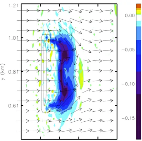
Fig. 8. X-Y section of wind vector at 18 m and pressure perturba-tion 240 s after line igniperturba-tion, initialized with uniform wind profile. The fire develops two fingers due to wind direction inversion in the middle. From Jenkins et al. (2010).
deficiencies. During this experiment, the wind measurements were taken only upwind from the actual fire, and only at two levels. Therefore, they do not provide a full description of the vertical wind profile which may affect the fire rate of spread through the atmosphere-fire coupling (Jenkins et al., 2010), and they lack the information about the actual wind at the fire line. Since the coupled fire-atmosphere model computes the fire rate of spread based on the local wind, it is absolutely crucial for its validation to know not only the fire spread rate but also the local wind speed.
Fig. 9. X-Z section of wind vector and pressure perturbation at the centerline for the fire in Fig. 8. From Jenkins et al. (2010).
Fig. 10. Topography of the finest domain of the Meadow Creek fire simulation. From Beezley et al. (2010).
Another validation venue is the use of data from tar-geted experiments, arranged with our collaborators. Such experiments could be directed to answer specific questions about fire behavior, which SFIRE is not able to model at the moment, e.g., how does ignition from a small fire in grass be-have before the fire reaches the full wind-driven spread rate, predicted by Rothermel’s formula.
Finally, we plan to perform the overall evaluation of the model in real fire cases. We are currently working on the validation based on the observed fire perimeters during Har-manli fire (Bulgaria), Meadow Creek Fire (Colorado), and Witch fire (California). Unfortunately, in most real fire cases, no meteorological data directly at the fire are available, so the only available information that may be used for model evaluation is the final fire perimeter, and, in some cases, a progression of recorded perimeters.
Fig. 11. The finest domain in the Meadow Creek fire simulation 5 h after ignition. Unburned fuel is displayed as green, burned fuel as brown. The heat flux from the fire appears near the fire line. Arrows indicate the surface winds, while streamlines show the atmospheric winds flowing over the fire region. Visualization in MayaVi. From Beezley et al. (2010).
10 Conclusions
We have described the atmosphere-fire model consisting of WRF coupled with SFIRE. The software is publicly avail-able and it supports both ideal and real runs. Visualization and diagnostic utilities are available. Currently, the model is suitable for research and education purposes. Validation is in progress.
10.1 Additional features
Fig. 12. The top level domain in the Meadow Creek fire simulation 5 h after ignition. Streamlines show the winds blowing East, over the Rocky Mountains and South down the coast of California. Visualization in MayaVi. From Beezley et al. (2010).
future. Adding smoke from the fire to WRF is also under consideration. There are two possible approaches to imple-mentation of the smoke dispersion in WRF and SFIRE. The basic one would be to treat the smoke as a passive tracer ad-vected by the wind, while the more advanced (taking into account its chemical reactivity during its transport), would require a coupling between the SFIRE and WRF-Chem. A list of desired features and a record of the progress of the de-velopment are maintained at http://www.openwfm.org/wiki/ OpenWFM development notes.
10.2 Atmosphere
Rothermel’s spread model (Eq. 1) assumes wind as if the fire was not there. In practice, the wind was measured away from the fire. In a coupled model, however, the feedback on the fire is from the wind that is influenced by the fire. Clark et al. (2004) noted that the horizontal wind right above the fireline may even be zero, and proposed to take the wind from a spec-ified distance behind the fireline. Also, the strong heat flux from fire disturbs the logarithmic wind profile, and the rate of spread as a function of wind at a specific altitude may not be a good approximation; rather, the fire spread may depend more strongly on the complete wind profile (Jenkins et al., 2010) and on turbulence (Sun et al., 2009). The assumption of horizontal homogeneity in the Monin-Obukhov similar-ity theory is not satisfied here; the horizontal dimension of
the active part of fire is not orders of magnitude larger than the boundary layer height as required, and it may be in fact smaller. Another indication that the Monin-Obukhov theory may not apply for fires is a strong drop in the heat transfer in the case of strong temperature gradients, shown in our early tests.
Horizontal wind could be interpolated vertically to differ-ent heights for differdiffer-ent fuels like in CAWFE model, which takes the wind from different mesh levels for different fuels. However, here we follow a classical approach of Rothermel (1972) and Baughman and Albini (1980), where the wind speed is evaluated at the common 6.1 m height, and then con-verted to the mid-flame height using the fuel-specific wind correction factors.
10.3 Fire
The more recent Scott and Burgan (2005) fuel categories are more detailed than Anderson (1982) categories, they are sup-ported by BehavePlus, and fuel maps using them are avail-able from Landfire. But instead of describing additional cat-egories innamelist.fire, it may be more useful to sup-port the imsup-port of fuel files from BehavePlus, which is also well suited for editing and diagnosing fuel models. More ac-curate fuel models (Albini et al., 1995; Clark et al., 1996a), including those in BehavePlus, consider fuels to be mixtures of components with different burn times, which results in a different heat release curve.
While the spread rate of established fire in the simulation of the FireFlux experiment was reasonably close, the sim-ulated fire still arrived at the observation towers too soon (Kochanski et al., 2010), because it started too quickly. A better parametrization of the ignition process seems to be in order. The fire spread in the Meadow Creek fire simulation was also too fast, but for a different reason. It is well known that the actual spread rates of wildland fires tend to be lower than the spread rates in simulations, which are derived from laboratory experiments. This effect might be attributed to ir-regularities on scales not captured by the simulation (Finney, 1998, p. 34), including granularity of the fuel supply not re-flected in the data. Refining the semi-empirical model from detailed numerical simulations and parametrizing complex fire behavior are suggested important research areas.
The computation of the heat fluxes in Eqs. (4) and (5) does not take into account the evaporation of moisture present in the fuel, only the production of water by burning of hydro-carbons. This error is typically just few %, however, which is small in comparison with other uncertainties. As the fuel moisture content can be significant in some ecosystems, it will be treated explicitly in a future version of the code. The fuel models should be dynamic (with variable fuel moisture) as in BehavePlus. Coen (2005) added an explicit diurnal cy-cle for the moisture into CAWFE. Here, moisture content could be coupled with existing WRF land surface models, which could take into account air humidity and precipitation. The radiative and convective parts of the sensible heat flux should be treated differently. The release of surface heat and moisture into the atmosphere are already present in WRF soil models. Their scale, however, is different from the powerful heat release from a fire.
Spotting (secondary ignitions by wind-lofted firebrands) could be modeled as additional point igntions, created dy-namically. Deciding when and where the secondary igni-tions occur, however, would require stochastic approaches, possibly modeling the spotting location and frequency as a random variable dependent on the fire location, distance, and the wind, similarly as in Mandel et al. (2004a).
10.4 Numerical methods
In a numerical implementation, the level set method is global, unlike tracers, which move locally. In spite of the fact that the level set equation determines the fire spread locally from the spread rate at the fireline, the behavior of the fireline de-pends slightly on the wind, the fuel, and the level set function in certain other locations from previous time steps, because of the discretization errors and the artificial diffusion. This nonlocal behavior has not been practically significant, how-ever.
The fuel fraction calculation (18) can have significant er-ror in the fire mesh cells near the fireline, which will to some degree average out over the atmospheric mesh cells. Rigor-ous error analysis will be done elsewhere. We are currently testing an alternative method which is always first order in the sense that it is exact when the time from ignition and the level set function are linear in space. The alternative method is more computationally expensive, but, on the other hand, it might allow to decrease the fire mesh refinement ratio; with large meshes, it is possible to run against 32 bit integer limits. 10.5 Data assimilation
Data assimilation for wildland fires is an area of great in-terest. Methodologies for a reaction-diffusion model were proposed based on the ensemble Kalman filter (EnKF) and the particle filter (Mandel et al., 2004b). Unfortunately, sta-tistical perturbations can cause spurious fires, which do not dissipate. Combination of the EnKF with Tikhonov regular-ization alleviates the problem somewhat (Johns and Mandel, 2008; Mandel et al., 2009), but the resulting method is still not robust enough. A new method, called morphing EnKF and based on combined amplitude and displacement correc-tion (Beezley and Mandel, 2008), was shown to work with WRF and SFIRE (Mandel et al., 2009), and it is under con-tinued development (Mandel et al., 2010, 2011). We are not aware of any work elsewhere on data assimilation for a cou-pled fire-atmosphere model. Particle filters were proposed for discrete cell-based fire models (Bianchini et al., 2006; Gu et al., 2009), using fitness functions involving the area burned rather than intensities of physical variables.
Supplementary material related to this article is available online at:
http://www.geosci-model-dev.net/4/591/2011/ gmd-4-591-2011-supplement.zip.
Acknowledgements. The authors would like to thank John Micha-lakes for developing the support for the refined surface fire grid in WRF and information about WRF algorithms, Ned Patton for providing a copy of his prototype code, Janice Coen for providing a copy of CAWFE, liason with NCAR, and useful suggestions, and Volodymyr Y. Kondratenko for implementing the interpolation of ignition time in Sect. 3.5, as well as other assistance. Other contributions to the model are acknowledged by bibliographic citations in the text. We would like to thank also Mary Ann Jenkins for reading this paper and suggesting improvements. This research was supported by NSF grant AGS-0835579 and NIST Fire Research Grants Program grant 60NANB7D6144.
Edited by: D. Lawrence
References
Albini, F. A. and Reinhardt, E. D.: Modeling ignition and burning rate of large woody natural fuels, Int. J. Wildland Fire, 5, 81–91, doi:10.1071/WF9950081, 1995.
Albini, F. A., Brown, J. K., Reinhardt, E. D., and Ottmar, R. D.: Calibration of a Large Fuel Burnout Model, Int. J. Wildland Fire, 5, 173–192, doi:10.1071/WF9950173, 1995.
Anderson, H. E.: Aids to determining fuel models for estimating fire behavior, General Technical Report INT-122, US Department of Agriculture, Forest Service, Intermountain Forest and Range Ex-periment Station, available at: http://www.fs.fed.us/rm/pubs int/ int gtr122.html (last access: 4 July 2011), 1982.
Andrews, P. L.: BehavePlus fire modeling system: past, present, and future, Paper J2.1, 7th Symposium on Fire and Forest Me-teorology, available at: http://ams.confex.com/ams/pdfpapers/ 126669.pdf (last access: 4 July 2011), 2007.
Baughman, R. G. and Albini, F. A.: Estimating Midflame Wind-speeds, in: Proceedings, Sixth Conference on Fire and Forest Meteorology, Seattle, WA April 22–24, 1980, Society of Ameri-cal Foresters, Washington, DC, 88–92, 1980.
Beer, T.: The interaction of wind and fire, Bound.-Lay. Meteorol., 54, 287–308, 1991.
Beezley, J. D.: Importing High-resolution Datasets into Geogrid, Paper P2, 12th WRF Users’ Workshop, National Center for At-mospheric Research, June 20–24, 2011, 2011.
Beezley, J. D. and Mandel, J.: Morphing Ensemble Kalman Filters, Tellus, 60A, 131–140, doi:10.1111/j.1600-0870.2007.00275.x, 2008.
Beezley, J. D., Kochanski, A., Kondratenko, V. Y., Mandel, J., and Soused´ık, B.: Simulation of the Meadow Creek fire using WRF-Fire, Poster at AGU Fall Meeting 2010, available at: http://www. openwfm.org/wiki/File:Agu10 jb.pdf (last access: 4 July 2011), 2010.
Benech, B.: Experimental Study of an Artificial Convective Plume Initiated from the Ground, J. Appl. Meteorol., 15, 127–137,
doi:10.1175/1520-0450(1976)015<0127:ESOAAC>2.0.CO;2, 1976.
Bianchini, G., Cort´es, A., Margalef, T., and Luque, E.: Im-proved Prediction Methods for Wildfires Using High Perfor-mance Computing: A Comparison, in: Computational Sci-ence, ICCS 2006, edited by: Alexandrov, V., van Albada, G., Sloot, P., and Dongarra, J., Vol. 3991 of Lecture Notes in Computer Science, Springer Berlin / Heidelberg, 539–546, doi:10.1007/1175850173, 2006.
Clark, T. L., Jenkins, M. A., Coen, J., and Packham, D.: A Coupled Atmospheric-Fire Model: Convective Feedback on Fire Line Dynamics, J. Appl. Meteorol., 35, 875–901, doi:10.1175/1520-0450(1996)035<0875:ACAMCF>2.0.CO;2, 1996a.
Clark, T. L., Jenkins, M. A., Coen, J. L., and Packham, D. R.: A coupled atmosphere-fire model: Role of the convective Froude number and dynamic fingering at the fireline, Int. J. Wildland Fire, 6, 177–190, doi:10.1071/WF9960177, 1996b.
Clark, T. L., Coen, J., and Latham, D.: Description of a Cou-pled Atmosphere-Fire Model, Int. J. Wildland Fire, 13, 49–64, doi:10.1071/WF03043, 2004.
Clements, C. B., Zhong, S., Goodrick, S., Li, J., Potter, B. E., Bian, X., Heilman, W. E., Charney, J. J., Perna, R., Jang, M., Lee, D., Patel, M., Street, S., and Aumann, G.: Observing the dynamics of wildland grass fires – FireFlux – A field validation experiment, Bull. Am. Meteorol. Soc., 88, 1369–1382, doi:10.1175/BAMS-88-9-1369, 2007.
Coen, J. L.: Simulation of the Big Elk Fire using coupled atmosphere-fire modeling, Int. J. Wildland Fire, 14, 49–59, doi:10.1071/WF04047, 2005.
Coen, J. L. and Patton, N.: Implementation of Wildland Fire Model Component in the Weather Research and Forecasting (WRF) Model, available at: http://www.mmm.ucar.edu/research/ wildfire/wrf/wrf summary.html (last access: December 2010), 2010.
Dobrinkova, N., Jordanov, G., and Mandel, J.: WRF-Fire Applied in Bulgaria, in: Numerical Methods and Applications, edited by Dimov, I., Dimova, S., and Kolkovska, N., vol. 6046 of Lecture Notes in Computer Science, Springer, Berlin/Heidelberg, 133– 140, doi:10.1007/978-3-642-18466-615, 2011.
Dudhia, J.: The Weather Research and Forecasting Model: 2010 Annual Update, 2010 WRF Users Workshop, available at: http://www.mmm.ucar.edu/wrf/users/workshops/WS2010/ abstracts/1-1.pdf (last access: 4 July 2011), 2010.
Filippi, J. B., Bosseur, F., Mari, C., Lac, C., Moigne, P. L., Cuenot, B., Veynante, D., Cariolle, D., and Balbi, J.-H.: Cou-pled atmosphere-wildland fire modelling, J. Adv. Model. Earth Syst., 1, Art. 11, doi:10.3894/JAMES.2009.1.11, 2009. Finney, M. A.: FARSITE: Fire Area Simulator-model development
and evaluation, Res. Pap. RMRS-RP-4, Ogden, UT: U.S. Depart-ment of Agriculture, Forest Service, Rocky Mountain Research Station, available at: http://www.fs.fed.us/rm/pubs/rmrs rp004. html (last access: 4 July 2011), 1998.