www.geosci-model-dev.net/8/1645/2015/ doi:10.5194/gmd-8-1645-2015
© Author(s) 2015. CC Attribution 3.0 License.
A spectral nudging method for the ACCESS1.3 atmospheric model
P. Uhe1,2and M. Thatcher1
1CSIRO Oceans and Atmosphere Flagship, 107–121 Station St, Aspendale, VIC 3195, Australia 2Environmental Change Institute, University of Oxford, Oxford, UK
Correspondence to: P. Uhe ([email protected])
Received: 7 August 2014 – Published in Geosci. Model Dev. Discuss.: 8 October 2014 Revised: 5 May 2015 – Accepted: 11 May 2015 – Published: 3 June 2015
Abstract. A convolution-based method of spectral nudging of atmospheric fields is developed in the Australian Commu-nity Climate and Earth Systems Simulator (ACCESS) sion 1.3 which uses the UK Met Office Unified Model ver-sion 7.3 as its atmospheric component. The use of convo-lutions allow for flexibility in application to different atmo-spheric grids. An approximation using one-dimensional con-volutions is applied, improving the time taken by the nudging scheme by 10–30 times compared with a version using a two-dimensional convolution, without measurably degrading its performance. Care needs to be taken in the order of the con-volutions and the frequency of nudging to obtain the best out-come. The spectral nudging scheme is benchmarked against a Newtonian relaxation method, nudging winds and air tem-perature towards ERA-Interim reanalyses. We find that the convolution approach can produce results that are competi-tive with Newtonian relaxation in both the effeccompeti-tiveness and efficiency of the scheme, while giving the added flexibility of choosing which length scales to nudge.
1 Introduction
Atmospheric modelling is a discipline that has impacts in many fields of scientific study as well as everyday life. For example, numerical weather prediction (Davies et al., 2005; Puri et al., 2013) provides us our daily weather forecasts and simulations of global climate (Taylor et al., 2012) give us forewarning of possible impacts of climate change. Global climate models are powerful tools, but they have limitations due to grid resolution, approximations to atmospheric phys-ical processes (e.g. convection and turbulent mixing), and also because of incomplete or imperfect data sets such as for representing land use. Furthermore, since the atmosphere
is a chaotic system, the simulated synoptic patterns deviate from observations over time. This makes it more difficult to evaluate modelled behaviour, since the advection of trac-ers depends on the synoptic-scale atmospheric circulation. In some cases, to reduce biases caused by these issues, it is use-ful to introduce a correction to align the model more closely with a host model, often an observational product such as the ERA-Interim reanalysis (ERAI; Dee et al., 2011). The process of adjusting dynamical variables of a model towards a host model is commonly known as nudging (Kida et al., 1991; Telford et al., 2008).
Nudging is useful for model development and scientific studies, where a more realistic atmospheric circulation can help determine errors or feedbacks in particular components of the model. Nudging in atmospheric models has been used to reduce the size of transport errors of trace gases for at-mospheric chemistry (Telford et al., 2008) and carbon cycle modelling (Koffi et al., 2012), dynamically downscaling to finer resolution (Wang et al., 2004), and generating regional analyses (von Storch et al., 2000). Two popular approaches to nudging in atmospheric models are Newtonian relaxation (Telford et al., 2008) and spectral nudging (Waldron et al., 1996).
using a cubic grid has previously been described by Thatcher and McGregor (2009). However, this paper differs from the previous work, as the scheme in ACCESS has been designed to exploit the symmetries of the ACCESS latitude–longitude grid. This paper also provides an extended analysis to com-pare the performance of various configurations of nudging using Newtonian relaxation and spectral nudging.
ACCESS is a numerical model designed to simulate Earth’s weather and climate systems. ACCESS is used for a wide range of applications from climate change scenarios and numerical weather prediction, to targeted scientific stud-ies into areas such as atmospheric chemistry and aerosols, and the carbon cycle. ACCESS is composed of a number of different submodels, of which the atmospheric component is the UK Met Office Unified Model (UM; Davies et al., 2005; The HadGEM2 Development Team, 2011). The version of ACCESS used in this study, ACCESS1.3, includes the Com-munity Atmosphere Biosphere Land Exchange model (CA-BLE; Kowalczyk et al., 2013) to represent the land surface. ACCESS often includes ocean and sea-ice components, but these components are not used in this study. A full descrip-tion of ACCESS can be obtained from Bi et al. (2013).
Nudging was originally implemented in the UM at the University of Cambridge, UK (Telford et al., 2008), using a Newtonian relaxation method. This applies a correction to the model at every time step, calculated from the differ-ence between the host model and the UM. The fields that are nudged are the key dynamical variables;2 (potential tem-perature),U(zonal wind) andV (meridional wind).
An alternate approach to Newtonian relaxation is spectral nudging (von Storch et al., 2000; Thatcher and McGregor, 2009; Waldron et al., 1996). The spectral nudging scheme builds upon and expands the already existing Newtonian re-laxation nudging code in the UM. It applies a low-pass spec-tral filter on the correction calculated as for the relaxation nudging, so the correction is only applied to large spatial scales. The spectral filter is applied using a convolution with a two-dimensional (2-D) Gaussian function. A convolution-based filter was chosen rather than using a more conventional discrete Fourier transform, as it is simple to implement a par-allel version within the UM framework and has the poten-tial to be generalized to irregular and limited area grids. It also operates on the physical distance between grid points, which makes it straight forward to apply consistently across the whole globe and does not require special treatment of the poles. Spectral nudging gives the flexibility of being able to nudge the large-scale features of the model towards the host, while allowing the small scales to be determined by the model’s own physics. Because of this, spectral nudging is particularly useful in regional climate modelling (Denis et al., 2002; Kanamaru and Kanamitsu, 2007; Kida et al., 1991) and dynamical downscaling (Liu et al., 2012). In these cases, the model resolution is finer than the host model, so there is no information to nudge the finest length scales of
the model towards, preventing the effective use of relaxation nudging.
The paper is structured as follows: Sect. 2 covers the im-plementation and configuration of nudging in ACCESS. This includes Sect. 2.1 covering relaxation nudging, then Sect. 2.2 describing the implementation of the spectral filter and the convolution method used to implement it. A 1-D filter that approximates the 2-D filter is described in Sect. 2.3. The 1-D filter gives significant improvements in the speed of calcu-lating the filter and reduces the amount of message passing. The set-up of the model used for simulations presented in this document is covered in Sect. 2.4.
The performance of the spectral nudging is analysed in Sect. 3. This is split up into subsections relating to dif-ferent indicators of its performance or looking at the be-haviour from different parameter choices. Section 3.1 com-pares nudged variables of the ACCESS model with ERAI, as well as the unconstrained fields of mean sea level pressure (MSLP) and precipitation. Section 3.2 compares the perfor-mance of the 1-D and 2-D spectral filters. Section 3.3 com-pares a number of different nudging configurations to see how closely they converge towards ERAI, and the effect of varying the spectral filter length scale. Lastly, Sect. 3.4 inves-tigates the effect of varying the period of nudging, comparing its effect on the temporal spectrum and run times.
2 Nudging implementation
The process of nudging aims at perturbing prognostic vari-ablesψmof a model (e.g. ACCESS) toward the correspond-ing variableψhof a host model (e.g. ERAI). The following section relates how nudging is implemented for each of the different methods used in this paper.
2.1 Newtonian relaxation
The standard Newtonian relaxation is applied by taking the difference betweenψm andψh,1ψ=ψm−ψh, and using this to correct the model,
ψm→ψm−α1ψ. (1)
over several model levels to reduce the discontinuity between the nudged and non-nudged regions. It can also be ramped down at the top of the atmosphere to avoid any conflict that may occur due to top boundary conditions of the model.
The code used for the relaxation nudging is based on code from Telford et al. (2008) with some modifications. The code was restructured to improve parallelism when spatially inter-polating host data and to use the ERAI data set as the host model instead of other reanalysis products.
2.2 Spectral nudging
Spectral nudging extends the Newtonian relaxation method by taking the correction term and applying a spectral (low-pass) filter so that large spatial wavelengths are adjusted while smaller wavelengths are left essentially unperturbed. The method chosen to do this is based on Thatcher and Mc-Gregor (2009), using a convolution of1ψ with a Gaussian function,w, to implement the filter. However, the approach in this paper differs from previous work in its application to the ACCESS grid, requiring different implementation of the convolution for different underlying grids.
The correction for spectral nudging is applied as follows:
ψm→ψm−α(1ψ∗w), (2)
where∗is the convolution operator. The convolution is cal-culated on the surface of a sphere (assumed to have radius R=1). This results in
1ψ∗w=
Z Z
1ψ (θ0, φ0)w(θ0−θ, φ0−φ)cos(φ0)dφ0dθ0 (3) where the Gaussian weighting function is
w(θ0−θ, φ0−φ)=1 bexp
−1σ2
2λ2
. (4)
λ is the standard deviation of the Gaussian function, which is referred to as the nudging length scale. θ andφ are the azimuthal angle and polar angle, respectively, andθ0andφ0 are dummy co-ordinates that are integrated over.b is a nor-malization factor,b=R Rexp−1σ2
2λ2
dφ0dθ0. Note thatbis evaluated after the expression is discretized.1σ (θ0−θ, φ0− φ)is the distance of a chord between the two points,(θ0, φ0) and(θ, φ):
1σ =2 arcsin
C
2
, (5)
where C(θ0−θ, φ0−φ) is the Cartesian distance between the points (θ0, φ0) and (θ, φ). Combining and discretizing Eqs. (3), (4) and (5), we get the correction that is applied by the scale-selective filter.
The ACCESS grid is horizontally decomposed into do-mains that are assigned to individual processors. The calcu-lation of the convolution at any point requires a global sum.
Global information is not stored on individual processors, so the message passing interface (MPI) is used to gather the1ψ arrays handled by each processor into a global array, and broadcast them to all processors. Each processor calculates the convolution just for its domain using this global informa-tion.
The naive implementation of the spectral filter involves a large computational effort (of orderN2computations for N horizontal grid points). A spectral filter could be imple-mented more efficiently via a fast Fourier transform (FFT), or a spherical harmonic transform, requiring orderNlog2N computations, but the convolution gives much greater flexi-bility to be used with different grid configurations, from the regular latitude–longitude grid to irregular or limited area grids. To mitigate the computational effort of the convolu-tion, a 1-D approximation to the convolution has been devel-oped, described in the following section.
2.3 1-D filter
To improve the computational efficiency of the spectral nudging scheme, the 2-D convolution can be separated into two 1-D convolutions, thereby reducing the computational effort to orderN3/2. The 2-D convolution is separated by splitting the Gaussian function into parts that depend solely on latitude or longitude. The two integrals in the 2-D filter can then be evaluated separately as two 1-D convolutions. The expression for the two 1-D convolutions is equal to the 2-D convolution on a flat Cartesian grid, but is an approxima-tion on a curved surface such as the global latitude–longitude grid.
w(θ0−θ, φ0−φ)≈1 bw(θ
0−θ, φ)w(θ0, φ0−φ) (6)
≈1
bexp
−1σ (θ0−θ, φ)2
2λ2
exp
−1σ (θ0, φ0−φ)2
2λ2
. (7)
A D convolution is applied in one direction, then another 1-D convolution is applied on the result of the first convolution. 1ψ∗w≈1
b[1ψ∗w(θ 0
, φ0−φ)]∗w(θ0−θ, φ) (8)
≈1
b
Z Z
w(θ0, φ0−φ)1ψ (θ0, φ0)cos(φ0)dφ0
·w(θ0−θ, φ)dθ0. (9)
data passed from processors associated with the same rows or columns of the horizontal grid.
Using this 1-D approximation, there is a choice in which convolution to apply first (i.e. either the zonal or meridional directions). Swapping the order of the integrals (convolu-tions) results in numerically different solutions. It is found that to reduce the error it is best to apply the convolution first along the latitudinal direction, then longitudinally. This is discussed in Sect. 3.2, which compares the different order-ings of the 1-D filter with the 2-D filter.
It also needs to be noted that the 1-D spectral filter is de-pendent on the model grid and the way the grid is decom-posed into domains for each processor. The configuration of the ACCESS grid allows for the convolution to be computed along rows of equal latitude or longitude and for those results to be efficiently distributed to rows or columns of processors. This approach needs to be modified for grids which do not have these symmetries. See Thatcher and McGregor (2009) for an example of a 1-D spectral filter applied on a cubic grid. 2.4 Model configuration/description
This paper uses simulations of ACCESS, in the ACCESS1.3 atmosphere-only configuration (Bi et al., 2013). This uses the atmospheric model UM vn7.3, CABLE 1.8 (Kowal-czyk et al., 2013), as well as prescribed sea-surface tem-peratures and sea-ice concentrations. The model horizontally uses a N96 grid (uniform latitude longitude grid with 1.875◦ east–west and 1.25◦north–south resolution). It has 38 ver-tical levels which are terrain following hybrid height levels, representing heights from 10 m to 36 km. The model was run with a 30 min time step.
A series of 1-year simulations were run, starting from 1 January 1990, each initialized in the same state, from a pre-vious climate simulation, i.e. with an initial state unrelated to any historical synoptic patterns. The only differences be-tween simulations were in the nudging configuration. These short experiments were chosen to evaluate the performance of different nudging methods and choice of nudging param-eters. Longer climate simulations may also provide more in depth insight into biases in the nudging scheme, but this eval-uation is beyond the scope of this paper.
The nudging component used the ERAI reanalysis product as the host model, provided at 6 hourly intervals. The ERAI data was linearly interpolated temporally to each time step. It was interpolated horizontally using bi-cubic interpolation, from its native 0.75◦east–west and 0.75◦ north–south to a resolution of 1.875◦east–west by 1.25◦north–south, match-ing the grid used by the ACCESS1.3 atmosphere. This is a higher resolution than the ERA-40 reanalysis used in Telford et al. (2008) of 3.75◦east-west by 2.5◦north–south.
The ERAI data set was interpolated vertically to the AC-CESS1.3 model levels, using the vertical interpolation de-veloped in Telford et al. (2008), based on a piece-wise lin-ear interpolation with respect to the natural logarithm of the
air pressure. Some nudging methods include corrections to the vertical interpolation to account for the differences in orography between the simulation model and the host model (ACCESS1.3 and ERAI in this paper, respectively), such as exploiting the lapse rate to correct the interpolation of air temperature. However, since our goal in this manuscript is to evaluate the scale-selective filter compared to Newtonian re-laxation, we have elected to retain the original interpolation scheme of Telford et al. (2008) for this study. Nevertheless, orographic adjustment for interpolated fields is an important topic that we intend to address in further work.
Nudging was applied to potential temperature (2), zonal wind (U) and meridional wind (V). The choice of which prognostic variables to nudge is an important aspect of the experiment design. Kanamaru and Kanamitsu (2007) argued that the U and V wind components, temperature, water vapour and surface pressure, all needed to be nudged to suffi-ciently constrain the large-scale biases of the model. Jeuken et al. (1996) also highlighted the effect nudging can have on the model physics if the nudging terms become too large. For simplicity, we have chosen to nudge the2,U, andV so as to be consistent with the nudging approach used by Telford et al. (2008). Note that we specifically avoid nudging the wa-ter vapour due to its potentially highly non-linear behaviour in the presence of clouds. We specifically consider whether the nudging is unbalancing the model in Sect. 3.4 in the con-text of the temperature temporal spectra.
The nudging adjustment was only applied from vertical level 7, corresponding to about 1 km in height above the sur-face terrain. The nudging amplitudeαwas ramped up from 0 to the full strength over three vertical levels so as to reduce the discontinuity between nudged and non-nudged parts of the atmosphere.αwas also ramped down over the top three vertical levels of the model.
The parameters varied in the experiments were the nudg-ing method, nudgnudg-ing period, maximum nudgnudg-ing strength, and spectral filter length. The relaxation nudging is always applied every time step, and the spectral filter can be applied at frequencies that are multiples of the time step and divide into 6 h (e.g. 0.5, 1, 2, 3 or 6 h). Most spectral nudging sim-ulations analysed in this manuscript have nudging applied at a frequency of 1 h, which is justified in Sect. 3.4.
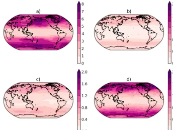
Figure 1. Spatial distributions of the RMSE in air temperature of ACCESS simulations. This is measured in Kelvin on a 2-D horizontal plane at 250 hPa and averaged over 1-year simulations excepting the first 10 days. (a) is the control with no nudging. (b) is the relaxation nudging with hard nudging. (c and d) are spectral nudging using the 1-D filter with hard nudging, applied once an hour. Different nudging length scales were used:λ=0.1 in (c) andλ=0.2 in (d). Note, for clarity, (a) uses a different scale for the contours.
3 Results and discussion
To determine the performance of the spectral filter, we look at the nudged runs compared with ERAI, as well as comparing with a control simulation without nudging. The control sim-ulation also gives an indication of the behaviour of the nudg-ing tendencies that were required to change the evolution of the simulation. The analysis was conducted on the nudged air temperature and wind fields, measured on planes of con-stant pressure at 250, 500 and 850 hPa. Note that although the potential temperature2is nudged, we actually evaluate the air temperatureT when comparing the simulated results with ERAI. Two unconstrained fields, MSLP and precipita-tion, were also evaluated. Except where specified otherwise, the whole 1-year simulations excepting the first 10 days was used. Excluding this period from the analysis ensures the at-mosphere is settled fully into the nudged state.
After describing the impact of nudging in Sect. 3.1, we compare different implementations of the 1-D and 2-D spec-tral filters in Sect. 3.2 and then evaluate the influence of us-ing different spectral filter parameters in Sect. 3.3. Lastly, Sect. 3.4 gives a justification for the selection of the period of application of spectral nudging which is used throughout this manuscript.
3.1 Analysis of mean state and variance in the nudged model
3.1.1 Effect of nudging on nudged atmospheric fields Figure 1 shows the spatial distribution of the root mean squared error (RMSE) at 250 hPa for different ACCESS sim-ulations, where we are defining the error as the difference between ACCESS and ERAI. It is calculated over a 1-year simulation, excepting the first 10 days, for the 6 hourly inter-vals the ERAI data is provided on. For these plots, a control simulation with no nudging is compared against simulations using relaxation nudging and spectral nudging. The different behaviour between the nudged and control simulations pro-vides an indication of the strength of the nudging tendencies. The 1-D filter was chosen as the preferred method of spectral nudging, as discussed further in Sect. 3.2. In all cases, the nudged runs have much smaller errors than the control simu-lation, indicating closer agreement with ERAI. The spectral filter with small length scales nudged (Fig. 1c) results in be-haviour similar to the relaxation nudging (Fig. 1b). As the filter length scale is increased, larger wavelengths are able to deviate from ERAI, and the magnitudes of the deviations are larger (Fig. 1d).
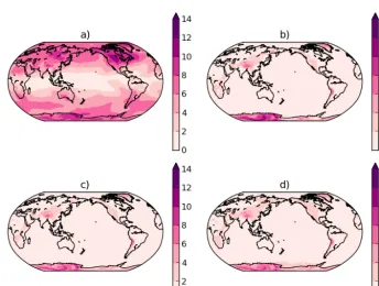
Figure 2. Spatial distributions of the RMSE in air temperature of ACCESS simulations. This is measured in Kelvin on a 2-D horizontal plane at 500 hPa and averaged over 1-year simulations excepting the first 10 days. (a) is the control with no nudging. (b) is the relaxation nudging with hard nudging. (c and d) are spectral nudging using the 1-D filter with hard nudging, applied once an hour. Different nudging length scales were used:λ=0.1 in (c) andλ=0.2 in (d). Note, for clarity, (a) uses a different scale for the contours.
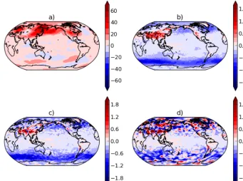
Figure 4. Spatial distributions of the difference in variance of air temperature between ACCESS simulations and ERAI. This is measured in Kelvin squared, on a 2-D horizontal plane at 500 hPa and averaged over 1-year simulations excepting the first 10 days. (a) is the control with no nudging. (b) is the relaxation nudging hard nudging. (c and d) are spectral nudging using the 1-D filter with hard nudging, applied once an hour. Different nudging length scales were used:λ=0.1 in (c) andλ=0.2 in (d). Note, for clarity, (a) uses a different scale for the contours.
the simulation over high orographic features such as the Hi-malayas, Antarctica or the Andes. These differences become more pronounced with the 850 hPa results, which is close to the lowest atmospheric levels that are nudged. We would expect there to be some differences between ACCESS and ERAI near the surface due to different representation of land-surface processes and different boundary layer parametriza-tions between the different atmospheric models. However, the largest errors are located where there is likely to be a mismatch in orographic height between ACCESS and ERAI and may suggest a limitation of the current method of inter-polating ERAI to the ACCESS grid.
The U andV winds show similar trends in the relative RMSE between different simulations as those shown for tem-perature in Figs. 1, 2 and 3. This is demonstrated by the global average RMSE of these fields, shown in Tables 2 and 3. These tables present data at atmospheric levels of 250, 500 and 850 hPa. We note that all of the nudging simulations are more strongly constrained in RMSE than the control simula-tion with no nudging. This is true for each of the variables, at each level. At 850 hPa, which is close to the lowest atmo-spheric levels that are nudged, theU andV winds have an average RMSE similar to the higher atmospheric levels. In contrast, the air temperature average RMSE shown in Fig. 1 is multiple times greater than the higher atmospheric lev-els. This shows that temperature is more affected by the
sur-face and orographic differences. We also note that the hard nudging simulations are more constrained in RMSE than the equivalent simulations with soft nudging in all cases.
Since we intend to use the nudging in the simulation over climate timescales (i.e. decades), it is useful to determine how well the simulation predicts the variance as well as the mean air temperature. Figure 4 shows the differences in the variance of air temperature between the ACCESS simula-tions and ERAI at 500 hPa. Note that ACCESS consistently overestimates the variance of the air temperature in the con-trol experiment compared to ERAI (Fig. 4a), presumably as a consequence of imperfect physical parametrizations. We note that this overestimate of the variance in air temperature is reduced by the nudging, with the difference in variance for Fig. 4b–d being an order of magnitude less than for Fig. 4a.
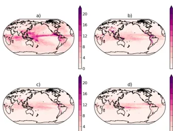
Figure 5. Spatial distributions of the RMSE for MSLP in hectopascal, between ACCESS simulations and ERAI. This is averaged over daily mean values for 1-year simulations excepting the first 10 days. (a) is the control with no nudging. (b) is the relaxation nudging hard nudging. (c and d) are spectral nudging using the 1-D filter with hard nudging, applied once an hour. Different nudging length scales were used:
λ=0.1 in (c) andλ=0.2 in (d).
Table 1. Comparison of RMSE and GAE in air temperature measured in Kelvin, for 1-year simulations excepting the first 10 days, using different nudging methods. Spectral nudging experiments use nudging applied once an hour.
Experiment RMSE GAE
250 hPa 500 hPa 850 hPa 250 hPa 500 hPa 850 hPa
Control 4.25 4.69 5.08 −0.37 0.13 0.39
Relaxation, soft 0.42 0.38 1.37 0.030 0.033 0.27
Relaxation, hard 0.32 0.26 1.39 0.15 0.073 0.39
Spectral, soft,λ=0.1 0.68 0.64 1.55 −0.026 −0.042 0.13 Spectral, hard,λ=0.03 0.35 0.29 1.37 0.13 0.057 0.37 Spectral, hard,λ=0.1 0.45 0.41 1.36 0.081 −0.001 0.18 Spectral, hard,λ=0.2 0.90 0.83 1.62 0.063 −0.021 0.11
Table 2. Comparison of RMSE and GAE inU measured in metres per second, for 1-year simulations excepting the first 10 days, using different nudging methods. Spectral nudging experiments use nudging applied once an hour.
Experiment RMSE GAE
250 hPa 500 hPa 850 hPa 250 hPa 500 hPa 850 hPa
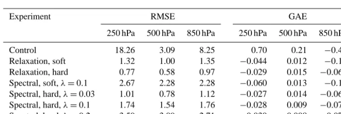
Control 18.26 3.09 8.25 0.70 0.21 −0.42
Relaxation, soft 1.32 1.00 1.35 −0.044 0.012 −0.12 Relaxation, hard 0.77 0.58 0.97 −0.029 0.015 −0.068 Spectral, soft,λ=0.1 2.67 2.28 2.28 −0.060 0.013 −0.12 Spectral, hard,λ=0.03 1.01 0.78 1.12 −0.027 0.014 −0.068 Spectral, hard,λ=0.1 1.74 1.54 1.76 −0.028 0.009 −0.072 Spectral, hard,λ=0.2 3.59 3.09 2.71 −0.030 0.008 −0.072
than settle down to a constant value. For example, the mean GAE of air temperature at 250 hPa for the control simulation is −0.37 K but its standard deviation is 0.7 K. The nudged simulations, which have lower mean GAE, also have a cor-responding lower standard deviation of GAE of 0.01–0.04 K. This shows smaller fluctuations in the GAE of the nudged simulations and the control simulation.
Tables 1, 2 and 3 also show that the simulations that are more tightly constrained in RMSE do not necessarily re-sult in lower GAE. This is very dependant on the variable and vertical level looked at. For example, looking at V at 500 hPa in Table 3, the hard nudging simulations which are more constrained in RMSE have a lower GAE than the con-trol, whereas the soft nudging simulations are not noticeably improved relative to the control simulation. However, forV at 250 hPa, the GAEs for all of the nudged simulations are reduced by an order of magnitude relative to the control sim-ulation and there is very little difference between the nudged simulations. The GAE can also have the opposite trend to the RMSE. An example of this is forT in Table 1, where the hard relaxation nudging has a smaller RMSE but a larger magni-tude of GAE compared to the hard spectral nudging simula-tions. Hence, there is no nudging approach that clearly pro-duces superior GAE results for all measures. However, the GAE for nudging simulations is comparable or lower than
the control simulations for all cases, and there are only a few values that are not improved when nudging is introduced. 3.1.2 Effect of nudging on unconstrained
atmospheric fields
Table 3. Comparison of RMSE and GAE inV measured in metres per second, for 1-year simulations excepting the first 10 days, using different nudging methods. Spectral nudging experiments use nudging applied once an hour.
Experiment RMSE GAE
250 hPa 500 hPa 850 hPa 250 hPa 500 hPa 850 hPa
Control 18.0 11.7 7.84 −0.061 0.021 −0.034
Relaxation, soft 1.47 1.09 1.34 0.006 0.020 0.003
Relaxation, hard 0.92 0.70 1.00 0.006 0.011 0.004
Spectral, soft,λ=0.1 2.63 2.21 2.16 0.006 0.022 0.001 Spectral, hard,λ=0.03 1.16 0.91 1.14 0.007 0.013 0.007 Spectral, hard,λ=0.1 1.72 1.47 1.65 0.007 0.014 0.012 Spectral, hard,λ=0.2 3.47 2.96 2.57 0.006 0.016 0.011
MSLP RMSE is similar for each of the nudged simulations, although MSLP is a relatively smooth field and can be less sensitive to smaller-scale differences in the nudging.
In Fig. 6 we consider the RMSE of the monthly mean rainfall. To cover the whole seasonal cycle, the 1-year sim-ulation including the first 10 days was used in this analysis. As the ERAI precipitation is calculated by a model with dif-ferent physics to ACCESS1.3, differences in specific rainfall events are expected. Due to this and the significant spatial and temporal variability in rainfall, the monthly mean values were chosen to provide a more consistent interpretation of precipitation biases than comparing higher frequency data. This only allows us to evaluate the spatial distribution of the rainfall rather than the timing of rainfall events. Each of the nudged simulations have improved the monthly precipitation compared to the control simulation. However, Fig. 6b shows a worsening of the RMSE for the hard relaxation method over a few limited regions such as the Himalayas and An-des compared to the control simulation (Fig. 6a). This is-sue is also present in the soft relaxation nudging simulation (not shown) and this result is consistent with Zhang et al. (2014), who found that Newtonian relaxation could have a detrimental effect on the cloud and precipitation processes due to temperature nudging. However, Fig. 6c and d, using spectral nudging, have reduced this issue or even removed the problem in some locations. It is clear that leaving smaller length scales unperturbed by the spectral filter is advanta-geous for the model physical parametrizations at least when simulating rainfall processes, even for the relatively strong nudging case shown in Fig. 6.
3.2 Evaluation of 1-D filter approximation
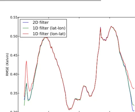
The majority of results presented in this manuscript are for nudging simulations using the 1-D filter. To justify this choice of spectral filter method, in this section we compare the results of different configurations of the 1-D filter to those obtained using the 2-D filter. There are two ways to order the convolutions in the 1-D filter, with the zonal convolution fol-lowed by the meridional convolution (1-D filter, long–lat), or
100 50 0 50 100
Latitude (degrees) 0.30
0.35 0.40 0.45 0.50 0.55
RMSE (Kelvin)
2D filter
1D filter (lat-lon)
1D filter (lon-lat)
Figure 7. RMSE of air temperature at 500 hPa, of 1-D filters and 2-D filter compared to ERAI. Data was averaged temporally and zonally, for 1 year (excepting from the first 10 days) of data sampled every 6 h. Each simulation uses the same nudging parameters, with hard nudging, using a filter length scale ofλ=0.1, applied once an hour.
the meridional convolution followed by the zonal convolu-tion (1-D filter, lat–long).
The RMSE of air temperature at 500 hPa is very similar between the different methods of spectral nudging. Simula-tions using hard nudging and a filter length ofλ=0.1 applied once an hour give an RMSE of 0.407 K for the 2-D filter and the 1-D filter lat–long, compared to 0.408 K for the 1-D filter long–lat, in air temperature at 500 hPa, over a 1-year simula-tion (excepting the first 10 days).
0 50 100 150 200 250 300 350 400 Days of simulation
0.0 0.5 1.0 1.5 2.0
Temperature RMSE (Kelvin)
Relaxation, soft
Spectral, soft,
λ=.1Relaxation, hard
Spectral, hard,
λ=.03Spectral, hard,
λ=.1Spectral, hard,
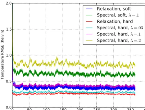
λ=.2Figure 8. RMSE of temperature at 500 hPa, for a 1-year simulation. Simulations of relaxation and spectral nudging are compared, with strong or weak nudging, and several different spectral filter length scales. All of the spectral nudging simulations use the 1-D filter nudged once an hour.
The difference between the long–lat and the lat–long ver-sion of the 1-D filter occurs because the grid points near the pole are physically close together in the longitudinal direc-tion. A small error at the pole could be spread zonally across multiple grid points. In the long–lat case, this error will re-main after the initial zonal convolution. On the other hand, when the meridional convolution is applied first, the error near the poles can be reduced. This is because the values at grid boxes close to the poles have a smaller weighting in the meridional convolution, as they have a smaller area.
As the 1-D filter constrains the model to a similar extent as the 2-D filter, with much reduced computational effort, it is clearly the preferred choice. The 1-D filter with the merid-ional convolution applied first has better performance at the poles, so it is the optimum configuration. All simulations us-ing spectral nudgus-ing refer to this configuration, except where specified otherwise.
3.3 Performance of the spectral filter
Figure 8 shows time series of RMSE of air temperature at 500 hPa for relaxation and spectral nudging simulations, us-ing different filter length scales and e-folding times. Each spectral nudging simulation uses hourly nudging as dis-cussed in Sect. 3.4. The convergence of RMSE depends on the combination of the e-folding time and nudging length scale (for the spectral nudging). The model is more tightly constrained using the shorter e-folding time (hard nudging) and smaller nudging length scales. The spectral filter with λ=0.1 and a 1 h e-folding time gives a RMSE similar to the relaxation nudging with a 6 h e-folding time. The more tightly constrained simulations reach a steady state more
quickly, and all the simulations shown have reached a steady RMSE within 4 days of simulation or less (not visible for the timescale of this plot).
Tables 1, 2 and 3 show the temporally and spatially aver-aged RMSE and GAE for each of the nudged fieldsT,Uand V at 250, 500 and 850 hPa levels. The simulations shown in these tables have the same relationship in RMSE as shown in Fig. 8. In particular, for a given strength of nudging, the re-laxation nudging has the smallest RMSE, the spectral nudg-ing withλ=0.03 is closest to the relaxation nudging, and the RMSE increases for the spectral nudging as the filter length increases. This is true for each of the variablesT,U andV, at each level evaluated. In addition, the hard nudging simula-tions result in smaller RMSE than the equivalent set-up using soft nudging.
As seen in Sect. 3.1.1, the GAE is generally improved in comparison to the control simulation. In addition, the hard spectral nudging with the smallest filter length, λ=0.03, produces GAEs that are reasonably consistent with the relax-ation nudging results. However, when comparing the differ-ent nudging methods, there is no clear pattern across levels and variables. For hard nudging, the spectral filter simula-tions have a smaller temperature GAE at all levels compared to the relaxation nudging, but the same is not the case when looking at the soft nudging simulations or when evaluatingU andV. Hence, there is no clear advantage of any particular nudging method when evaluating the model performance in terms of GAE.
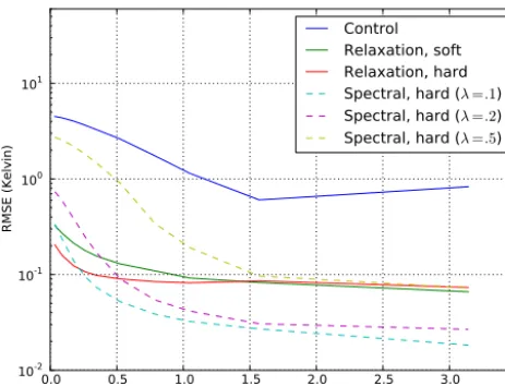
To further show the effect of the spectral filter at different length scales, the simulation output was re-gridded to a range of coarser resolutions. Re-gridding to coarser resolutions re-moves the fine-scale detail in a similar way to the spectral fil-ter, so the performance of the spectral filter should improve at coarser resolutions. This is shown in Fig. 9, which com-pares the RMSE at different re-gridded resolutions for differ-ent simulations.
0.0 0.5 1.0 1.5 2.0 2.5 3.0 3.5 Resolution (radians)
10-2 10-1 100 101
RMSE (Kelvin)
Control
Relaxation, soft
Relaxation, hard
Spectral, hard (
λ=.1)
Spectral, hard (
λ=.2)
Spectral, hard (
λ=.5)
Figure 9. Plot of average RMSE of temperature at 500 hPa, at dif-ferent regridded resolutions, for various simulations using nudging and a control simulation without nudging. All of the spectral nudg-ing simulations use the 1-D filter nudged once an hour.
3.4 Nudging period
Figure 10 shows the temporal spectra of the 500 hPa air tem-perature from simulations using different nudging configura-tions. Relaxation nudging is applied every time step, so the nudging period is only applicable to the spectral filter. Nudg-ing can be applied at intervals from every time step (30 min), to the period of the host data (6 h in the case of ERAI).
All valid choices of nudging period are able to sufficiently constrain the model, given a comparablee-folding time. The choice of nudging, therefore, is a trade-off between computa-tional effort and increased nudging shock, as constraining the model when nudging less frequently requires larger adjust-ments to the perturbed field. Nudging less frequently hence causes distortions to the temporal spectra as shown in Fig. 10. However, less frequent nudging offers a significant speedup as discussed below.
Examining Fig. 10 in more detail, it is evident that nudg-ing with a period of 6 h results in spikes in the Fourier spec-trum at certain frequencies. This shows that the nudging ad-justment is unbalancing the atmospheric model, causing it to respond unevenly in the spectrum. When nudging every hour, these imbalances are removed. Apart from a distortion in the spectrum below half an hour (one time step), the line for spectral nudging every hour lies on top on the line for spectral nudging at every time step.
The spectra when nudging every time step is qualitatively similar to the control simulation but shifted down in magni-tude. The spectral nudging at every time step has a spectrum in between the curves for the control and relaxation nudg-ing. The spectrum for the 2-D filter is indistinguishable to the equivalent simulations using the 1-D spectral filter with the same filter length scale (2-D filter not shown).
2 4 6 8 10 12 14
Period (hours) 101
102 103
Amplitude (Kelvin)
Control
Relaxation (every timestep)
Spectral (every timestep)
Spectral (every hour)
Spectral (every 6 hours)
Figure 10. Temporal Fourier spectra for temperature at 500 hPa, for simulations with different nudging periods. Soft nudging was applied and the spectral nudging simulations used a filter length scale ofλ=0.1.
Considering the speed benefits of different nudging fre-quencies, the 1-D spectral filter nudged every 6 h adds 3.3 % to the run time (the same as Newtonian relaxation). When the period is decreased to 1 h or 30 min this increases the run time by 6.7 and 12 %, respectively. The 2-D spectral filter in comparison adds 33 % when nudged every 6 h, increasing to 190 and 376 %, which is not viable for most uses.
Nudging at hourly intervals can be used as a compromise between speed of computation and reducing the distortions in the spectra, and is the standard period of nudging used for spectral nudging in this paper.
4 Conclusions
This paper has introduced the use of spectral nudging in the UM and ACCESS. This is achieved through a novel con-volution method, first described by Thatcher and McGregor (2009), but generalized in this paper for use with latitude– longitude grids as used by the ACCESS atmospheric model. Analysis of the different configurations of nudging shows that the nudging schemes effectively constrain the nudged fields to follow the host model (ERAI). We have surveyed the spectral filter across a range of filter length scales. The spec-tral nudging scheme approaches the Newtonian relaxation nudging when small length scales are nudged, but allows the flexibility to nudge only large spatial structures when the fil-ter length scale is increased.
the orographic height between the ACCESS simulation and ERAI, suggesting a problem with the vertical interpolation to the ACCESS grid used by the nudging. We intend to address this problem in future work.
We have also considered the implications of nudging on MSLP and precipitation, which are not directly perturbed by the nudging. MSLP is a reasonably smoothly varying field and is well constrained by the nudging in all simulations to agree with ERA-Interim. There are some differences under high orography, although this may be more related to the method used for calculating MSLP under orography rather than the nudging method. The nudged simulation improved the monthly mean rainfall compared to the control simu-lation. Furthermore, the spectral nudging simulations pre-dicted rainfall that was in closer agreement with ERAI than the relaxation nudging simulations. This provides an exam-ple of where the spectral filter can have an advantage over the Newtonian relaxation approach, particularly for physical processes that are sensitive to the local behaviour of the at-mosphere.
The 1-D spectral filter is shown to perform as well as the 2-D filter, while producing a speedup of 10–30 times. This is achieved by the approximation of separating the 2-D con-volution into 1-D concon-volutions and by using symmetries of the model grid to reduce communication between processors. We also identified that, due to the geometry of our grid, the order of convolutions in the 1-D filter was important. To re-duce error in the approximation, the meridional convolution is applied first.
Nudging with different frequencies was also investigated, showing that nudging every 6 h is still able to constrain the model, but introduces distortions to the spectra. Nudging once an hour produces a speedup in comparison to nudging every time step, while introducing minimal distortions, so it was used for the majority of simulations.
The approach used to implement the 2-D and 1-D spec-tral filters is applicable to many other models. The 2-D con-volution method can be implemented on any grid, though it suffers from being computationally expensive. The 1-D filter can be applied to irregular or more complex grids, but would require modification to separate the 2-D Gaussian function using an approximation that is appropriate for the particular grid.
Future work on spectral nudging in ACCESS will in-volve generalizing the spectral nudging to limited area and stretched grid configurations. Another potential approach to gaining a speedup in the convolution-based spectral filter is to compute the convolutions over a small neighbourhood, rather than the whole globe, ignoring areas where the Gaus-sian function has values close to 0. The ability to extend the convolution-based spectral filter within the ACCESS/UM framework and in other modelling systems is an advantage of this approach.
Code availability
Due to intellectual property right restrictions, CSIRO cannot publish the full source code for ACCESS or the UM. The Met Office Unified Model (UM) with the spectral nudging source code and configuration described in this paper can be obtained under an end-user license agreement (EULA) from CSIRO for educational and non-commercial research use for specific projects. To request a EULA for the modified UM, and/or to obtain the ACCESS1.3 model configuration used in this paper, please contact Tony Hirst ([email protected]).
Acknowledgements. Thanks to Peter Dobrohotoff, John
McGre-gor and Tony Hirst for their feedback in the preparation of the manuscript and the anonymous reviewers for suggested revisions to improve the manuscript. This research was undertaken with the assistance of resources from the National Computational Infras-tructure (NCI), which is supported by the Australian Government. This work included funding by the Australian Government through the Australian Climate Change Science Programme. ERA-Interim data, from the European Centre for Medium-Range Weather Forecasts (ECMWF) was used in this research. The UM was made available to CSIRO under the consortium agreement Met Office’s Unified Model Earth System Modelling software (Met Office Ref. L1587).
Edited by: G. Mann
References
Bi, D., Dix, M., Marsland, S., O’Farrell, S., Rashid, H., Uotila, P., Hirst, A., Kowalczyk, E., Golebiewski, M., Sullivan, A., Yan, H., Hannah, N., Franklin, C., Sun, Z., Vohralik, P., Watterson, I., Zhou, X., Fiedler, R., Collier, M., Ma, Y., Noonan, J., Stevens, L., Uhe, P., Zhu, H., Griffies, S., Hill, R., Harris, C., and Puri, K.: The ACCESS coupled model: description, control climate and evaluation, Aust. Met. Oceanogr. J., 63, 41–64, 2013.
Davies, T., Cullen, M. J. P., Malcolm, A. J., Mawson, M. H., Staniforth, A., White, A. A., and Wood, N.: A new dynami-cal core for the Met Office’s global and regional modelling of the atmosphere, Q. J. Roy. Meteorol. Soc., 131, 1759–1782, doi:10.1256/qj.04.101, 2005.
Dee, D. P., Uppala, S. M., Simmons, A. J., Berrisford, P., Poli, P., Kobayashi, S., Andrae, U., Balmaseda, M. A., Balsamo, G., Bauer, P., Bechtold, P., Beljaars, A. C. M., van de Berg, L., Bidlot, J., Bormann, N., Delsol, C., Dragani, R., Fuentes, M., Geer, A. J., Haimberger, L., Healy, S. B., Hersbach, H., Hólm, E. V., Isaksen, L., Kållberg, P., Köhler, M., Matricardi, M., McNally, A. P., Monge-Sanz, B. M., Morcrette, J.-J., Park, B.-K., Peubey, C., de Rosnay, P., Tavolato, C., Thépaut, J.-N., and Vitart, F.: The ERA-Interim reanalysis: configuration and perfor-mance of the data assimilation system, Q. J. Roy. Meteorol. Soc., 137, 553–597, doi:10.1002/qj.828, 2011.
Dix, M., Vohralik, P., Bi, D., Rashid, H., Marsland, S., O’Farrell, S., Uotila, P., Hirst, T., Kowalczyk, E., Sullivan, A., Yan, H., Franklin, C., Sun, Z., Watterson, I., Collier, M., Noonan, J., Rot-stayn, L., Stevens, L., Uhe, P., and Puri, K.: The ACCESS couple model: documentation of core CMIP5 simulations and initial re-sults, Aust. Met. Oceanogr. J., 63, 83–99, 2013.
Jeuken, A., Siegmund, P., Heijboer, L., Feichter, J., and Bengtsson, L.: On the potential of assimilating meteorological analyses in a global climate model for the purpose of model validation, J. Geophys. Res.-Atmos., 101, 16939–16950, 1996.
Kanamaru, H. and Kanamitsu, M.: Scale-selective bias correction in a downscaling of global analysis using a regional model, Mon. Weather Rev., 135, 334–350, 2007.
Kida, H., Koide, T., Sasaki, H., and Chiba, M.: A new approach for coupling a limited area model to a GCM for regional climate simulations, J. Meteorol. Soc. Jpn., 69, 723–728, 1991. Koffi, E. N., Rayner, P. J., Scholze, M., and Beer, C.:
At-mospheric constraints on gross primary productivity and net ecosystem productivity: results from a carbon-cycle data assimilation system, Global Biogeochem. Cy., 26, 1–15, doi:10.1029/2010GB003900, 2012.
Kowalczyk, E., Stevens, L., Law, R., Dix, M., Wang, Y., Harman, I., Haynes, K., Srbinovsky, J., Pak, B., and Ziehn, T.: The land sur-face model component of ACCESS: description and impact on the simulated surface climatology, Aust. Met. Oceanogr. J., 63, 65–82, 2013.
Liu, P., Tsimpidi, A. P., Hu, Y., Stone, B., Russell, A. G., and Nenes, A.: Differences between downscaling with spectral and grid nudging using WRF, Atmos. Chem. Phys., 12, 3601–3610, doi:10.5194/acp-12-3601-2012, 2012.
Puri, K., Dietachmayer, G., Steinle, P., Dix, M., Rikus, L., Lo-gan, L., Naughton, M., Tingwell, C., Xiao, Y., Barras, V., Bermous, I., Bowen, R., Deschamps, L., Franklin, C., Fraser, J., Glowacki, T., Harris, B., Lee, J., Le, T., Roff, G., Sulaiman, A., Sims, H., Sun, X., Sun, Z., Zhu, H., Chattopadhyay, M., and Engel, C.: Implementation of the initial ACCESS numerical weather prediction system, Aust. Met. Oceanogr. J., 63, 265–284, 2013.
Taylor, K., Stouffer, R. L., and Meehl, G. A.: An Overview of CMIP5 and the experiment design, B. Am. Meteorol. Soc., 93, 485–498, doi:10.1175/BAMS-D-11-00094.1, 2012.
Telford, P. J., Braesicke, P., Morgenstern, O., and Pyle, J. A.: Tech-nical Note: Description and assessment of a nudged version of the new dynamics Unified Model, Atmos. Chem. Phys., 8, 1701– 1712, doi:10.5194/acp-8-1701-2008, 2008.
Thatcher, M. and McGregor, J. L.: Using a scale-selective fil-ter for dynamical downscaling with the conformal cubic atmospheric model, Mon. Weather Rev., 137, 1742–1752, doi:10.1175/2008MWR2599.1, 2009.
The HadGEM2 Development Team: Martin, G. M., Bellouin, N., Collins, W. J., Culverwell, I. D., Halloran, P. R., Hardiman, S. C., Hinton, T. J., Jones, C. D., McDonald, R. E., McLaren, A. J., O’Connor, F. M., Roberts, M. J., Rodriguez, J. M., Woodward, S., Best, M. J., Brooks, M. E., Brown, A. R., Butchart, N., Dear-den, C., Derbyshire, S. H., Dharssi, I., Doutriaux-Boucher, M., Edwards, J. M., Falloon, P. D., Gedney, N., Gray, L. J., Hewitt, H. T., Hobson, M., Huddleston, M. R., Hughes, J., Ineson, S., In-gram, W. J., James, P. M., Johns, T. C., Johnson, C. E., Jones, A., Jones, C. P., Joshi, M. M., Keen, A. B., Liddicoat, S., Lock, A. P., Maidens, A. V., Manners, J. C., Milton, S. F., Rae, J. G. L., Rid-ley, J. K., Sellar, A., Senior, C. A., Totterdell, I. J., Verhoef, A., Vidale, P. L., and Wiltshire, A.: The HadGEM2 family of Met Of-fice Unified Model climate configurations, Geosci. Model Dev., 4, 723–757, doi:10.5194/gmd-4-723-2011, 2011.
von Storch, H., Langenberg, H., and Feser, F.: A spectral nudging technique for dynamical downscaling purposes, Mon. Weather Rev., 128, 3664–3673, 2000.
Waldron, K., Paegle, J., and Horel, J.: Sensitivity of a spectrally filtered and nudged limited-area model to outer model options, Mon. Weather Rev., 124, 529–547, 1996.
Wang, Y., Leung, L. R., McGregor, J. L., Lee, D.-K., Wang, W.-C., Ding, Y., and Kimura, F.: Regional climate modelling: progress, challenges and prospects, J. Meteorol. Soc. Jpn., 82, 1599–1628, 2004.