High-Dimensionality Graph Data Reduction
Based on a Proposed New Algorithm
Lamyaa Al-Omairi, Jemal Abawajy, Morshed U. Chowdhury and Tahsien
Al-Quraishi
School of Information Technology, Deakin University, Geelong, Victoria, Australia.
{lalomair,jemal.abawajy,morshed.chowdhury and talqurai}
@deakin.edu.au
Abstract
In recent years, graph data analysis has become very important in modeling data distribution or structure in many applications, for example, social science, astronomy, computational biology or social networks with a massive number of nodes and edges. However, high-dimensionality of the graph data remains a difficult task, mainly because the analysis system is not used to dealing with large graph data. Therefore, graph-based dimensionality reduction approaches have been widely used in many machine learning and pattern recognition applications. This paper offers a novel dimensionality reduction approach based on the recent graph data. In particular, we focus on combining two linear methods: Neighborhood Preserving Embedding (NPE) method with the aim of preserving the local neighborhood information of a given dataset, and Principal Component Analysis (PCA) method with aims of maximizing the mutual information between the original high-dimensional data sets. The combination of NPE and PCA contributes to proposing a new Hybrid dimensionality reduction technique (HDR). We propose HDR to create a transformation matrix, based on formulating a generalized eigenvalue problem and solving it with Rayleigh Quotient solution. Consequently, therefore, a massive reduction is achieved compared to the use of PCA and NPE separately. We compared the results with the conventional PCA, NPE, and other linear dimension reduction methods. The proposed method HDR was found to perform better than other techniques. Experimental results have been based on two real datasets.
1
Introduction
With the rapid advances in the use of internet techniques, massive amounts of various types of data are generated every millisecond. Such data include image data, video data, audio data, text data, the instrument measured data, daily transaction data, social network data, etc. [1-3]. In such
Volume 63, 2019, Pages 1–10
applications, these data are presented in high-dimensional format. For example, a 64 X 64 image can be represented mathematically as a vector in a 4,906-dimensional space, and the vector serves as input for other applications. On the other hand, because of the high-dimensionality, it is typically hard to process such data efficiently. In this case, dimensionality reduction is used to map a set of high-dimensional data into a low-high-dimensional space and in the process preserve the intrinsic structure in the original data. In other words, dimensionality reduction aims to construct an alternative low-dimensional representation of graph data to enhance readability and interpretability. The purpose of low-dimensional is to learn an optimal low-dimensional representation, which could find and capture the meaningful basic geometry and possible discrimination information of the high-dimensional data. This low-dimensional representation needs to be meaningful and faithful to the genuine data. In practical terms, dimensionality reduction is a pre-processing stage in several data reduction approaches. The graph is one of the applications widely employed for modeling complex data in various applications, for instance, recommender systems, web mining, social networks, bibliographical networks, telecommunications just to name a few [3, 4]. Large-scale graph analysis with plenty of nodes and edges is a challenging task [5]. In order to handle massive graph data efficiently, the first crucial issue is to reduce the dimensional space of the original data properly so that advanced analytic tasks, like pattern discovery, analysis, and prediction can be performed. For the purpose of reducing the dimensions in order to project high-dimensional data to a new representation in low-dimensional space a significant number of algorithms have been introduced including linear and nonlinear methods, for example, PCA, factor analysis (FA), linear discriminant analysis
(LDA)…etc.[1] are liner methods and local linear embedding (LLE), ISOMAP…etc. [2] are nonlinear methods. Linear dimensionality reduction techniques are mainly developed for non-graphical data structures. Thus, these classical linear techniques cannot sufficiently handle complex graph-structured data.
Taking into account these weaknesses, this paper aims to create an efficient linear dimensionality reduction algorithm for undirected graphs. The new method is a hybrid dimensionality reduction approach (HDR) based on the combination of PCA and NPE, to locate one transition matrix for both approaches then multiplying the original data with the obtained transition matrix. This will give a lower-dimensional representation, where each dimensionality reduction technique, has to find a matrix transformation. The accuracy of the suggested HDR approach was compared with other common linear dimension reduction methods, such as PCA, NPE, locality preserving projections (LPP), Multidimensional scaling (MDS), LDA, and FA. We used DBLP and arXiv dataset for our simulation experiments in MATLAB 2015b. Our simulation results indicate that the suggested technique can provide superior classification efficiency for link prediction in DBLP and arXiv datasets.
The remainder of the paper is organized as follows: In Section 2, related work is presented while in section 3, introduce dimensionality reduction, the Principal Component Analysis (PCA) and Neighborhood Preserving Projections (NPE) briefly. In Section 4, the proposed hybrid dimensionality reduction method is detailed. The Experiments and results are presented in Section 5. This is followed by the conclusion in Section 6.
2
Related work
This section reviews several algorithms, which employ data representations for the construction of a graph and which have close relationships with the approach we propose. The typically used PCA is a classical method for performing a linear mapping of the data so that the variation of the data in the low-dimensional representation is maximized. The basis of the PCA is the extraction of the axes on
can be very helpful in unsupervised learning, there is no assurance that the new axes are in line with the discriminatory features in a classification issue [6]. An additional method is to consider class information when extracting the feature. One method is to apply class separability criterion from
Fisher’s linear discriminant analysis (FLDA) in [7] which has its basis in a family of functions of scattering matrices: the within-class covariance, and the total covariance matrices. One of the problems here is to select the optimal subset of orthogonally converted features for consequent classification. Therefore, it is important to use PCA in order to search for the optimal subset of converted components, which enable the attainment of the optimal classification. Mykola et al.
combined PCA with Fisher’s linear discriminant analysis for PCA previous purposes. Precisely, in
this approach, the essential point was to enhance the parametric class conditional of FLDA by the addition of a few principal components (PCs), of the PCA method. However, FLDA, although utilizing class information, also has a crucial weakness due to its parametric nature. Note here, some of the extracted components cannot exceed the number of classes minus one. Furthermore, as it can be understood from its name, FLDA works mainly and exclusively for linearly separable classes.
On the other hand, the LDA method is considered a statistical dimensionality reduction algorithm. The LDA algorithm chooses the most favorable direction for classification, which is not necessarily the best. Therefore, Liang Tang et al. in [8] proposed two dimensionality reduction methods called LDA-PLS and ex-LDA-PLS by combining LDA with the partial least squares (PLS) technique where the PLS aims to develop components that obtain most of the information that is useful in the original data. It reduces the dimensionality of the regression problem by employing less number of components than the number of data variables, where the proposed methods use PLS to adapt the LDA projection direction. However, the proposed methods in the experiments have not achieved the best direction in the training set; this proves LDA-PLS and ex-LDA-PLS cannot obtain the best results in the small dataset. Authors in [9] merged two linear dimensionality reduction methods, LPP and PCA. In the merger method, they lessened the linear dimensionality reduction of microarray dataset by using LPP then extracted principal components by applying PCA. The results showed that clustering based on PCA-LPP performed better than n PCA. However, this strategy does not consider the practical method in reducing the dimensionality because their main focus was clustering. One of the aims of the PCA technique is to achieve the highest possible data reconstruction capability of the features, while the discriminant analysis (DA) method [10] aims to maximize the discriminatory power of the features. Although both methods involve the application of eigenvector decomposition on the covariance matrices to decorrelate features and therefore to extract the features, however, several researchers tend to DA for feature extraction because features discrimination is of utmost importance for classification. To improve the performance of PCA in extracting a compact feature set for classification, Jiang proposed a hybrid of the PCA and DA to reduce the discriminatory power of the extracted features. Even though this hybrid method shows greater effectiveness in extracting the discriminatory features, it still suffers from the common mean problems, which is one of the problems involving the LDA algorithm. On the other hand, Kwak and Pedrycz discussed in [11] the independent component analysis (ICA) method and applying it for face recognition. Usually, when applying ICA on face recognition, we obtain enhanced unsupervised learning and high-order statistics. Although the ICA technique has been shown to perform well, it may still be challenging to separate each class due to the large variance in lighting and facial expression.
class-specific information. Moon and Qi [12] presented the SVM-ICA algorithm. As dimensionality reduction methods divide into supervised and unsupervised methods, Support Vector Machine (SVM) method belongs to the supervised category, while the ICA is within the unsupervised learning methods. Authors merged both categories in a hybrid method which is SVM-ICA to preserve the high classification precision in lower dimensional space. However, studies later showed [13] that this method is statistically oriented and therefore, not too much can be expected in terms of reliability and computational simplicity.
However, in our paper, we offer an effective hybrid linear dimensionality reduction approach specifically for graph based on obtaining the transformation matrix to both PCA and NPE at the same time, and this hybrid method provided high classification accuracy in lower dimensional space for a large graph.
3
Dimensionality reduction
Statistical and machine learning have a challenging issue when they deal with high‐dimensional
data, and usually, the number of input variables is decreased prior to the successful application of a data mining algorithm. Dimension reduction projects high dimensional data onto a low-dimensional space [14] and can be separated into feature selection and feature extraction [15]. The analytical
procedures facilitating this reduction is called “dimensionality reduction techniques.” A significant
number of algorithms have been introduced for dimensionality reduction divided into linear and nonlinear methods. Nonlinear dimensionality reduction methods are commonly used for nonlinear data that needs to be reduced before being processed, and examples of nonlinear methods are Locally
Linear Embedding (LLE), ISOMAP…etc. Linear dimensionality reduction methods deal with data sets which have a linear relationship; for example, linear methods are PCA, Factor Analysis (FA),
Linear Discriminant Analysis (LDA)…etc. The linear dimensionality reduction problem can be explained as thus: consider the original data 𝑿 = {𝒙1, 𝒙2, … , 𝒙𝑚} in high dimensional space 𝑅𝑝.
Then, find a matrix 𝐴 which is the number of components of data. The main idea is the extraction of eigenvectors and eigenvalues. The eigenvectors with the highest eigenvalues are the principal components of the data set. Matrix 𝐴 converts the original data points into a new set of data points
𝒀 = {𝒚1, 𝒚2, … , 𝒚𝑚} in a low-dimensional space 𝑅𝑞 (𝑞 ≪ 𝑝), such that 𝑦𝑖“represents”𝑥𝑖,
where: 𝒚𝑖= 𝑨𝑇𝒙𝑖, (1).
In this paper, we focused on two common linear techniques namely, Principal Component Analysis (PCA) method which is a classical method of feature extraction that has been extensively utilized in the area of machine learning, and Neighborhood Preserving Projections (NPE) method, which is a recently suggested linear method to reduce dimensionality.
3.1
PCA dimensionality reduction method
𝑺 = 𝑿𝒊− 𝑿̅, 𝑖 = 1, . . 𝑛 (2)
Then calculates the covariance matrix 𝑪.. Since the data are 𝐷 dimensional, the covariance matrix will be 𝐷 × 𝐷
𝑪 = 𝐶𝑜𝑣(𝑿) =1
𝑛 ∑ 𝑺 𝑺 𝑇 𝑛
𝑖=1 (3)
In this stage, calculate the eigenvectors corresponding to the highest eigenvalues of the covariance matrix is done by the equation below:
𝑨 = 𝑒𝑖𝑔(𝑪) (4)
Hence, it can reduce the dimensions of 𝑿 by the final step of PCA. Since PCA is a linear technique, it forms a linear equation between the original dataset and new reduced data 𝒀 by using
“(1)”. The algorithmic method for PCA is formally stated by the steps shown below: 1- Given an original data 𝑿, 𝑿 = {𝒙1, 𝒙2, . . , 𝒙𝑛}.
2- Calculate the mean 𝑿̅ of the set 𝑿, then subtract the mean from each of the data points. 3- Compute the covariance matrix as the equation “(3)”.
4- Calculate the eigenvalues and eigenvectors of the covariance matrix “(4)”.
3.2
NPE dimensionality reduction method
Neighborhood retaining embedding (NPE) [17] is an unsupervised manifold reduced dimension method introduced in recent years. NPE embeds the original data to low dimensional space, in which the local neighborhood structure on the data manifold is retained. NPE retains the local manifold structure, differing from PCA which retains the global structure. Local structure means that each data point can be represented as a linear combination of its neighbors. Let 𝑿 = { 𝒙𝒊 ∈ 𝑅𝐷, 𝑖 = 1,2 … , 𝑁}
denotes the input data in 𝑅𝐷 space. NPE aims to seek an optimal transformation matrix 𝑨 to map the D-dimensional data point 𝑥𝑖onto d-dimensional data point 𝒚𝒊, {𝒚𝒊∈ 𝑅𝑑, 𝑖 = 1,2, … , 𝑁}; (𝑑 ≪ 𝐷),
namely , 𝒚𝒊= 𝑨𝑇𝒙𝒊(equation 1)in which the local neighborhood structure of the original data set 𝑿
can be retained. NPE first locates the neighbors of each data point in space 𝑅𝐷, then builds an
adjacency graph on the input data set. Let the weights 𝑾𝑖𝑗 be the coefficients that best reconstruct 𝒙𝑖
from its neighbors 𝑗 = 1,2, … , 𝐾, and 𝑾 = 𝑾𝑖𝑗 be the reconstruct matrix. The matrix 𝑾 can be
computed by reducing the objective function:
𝑾 = ∑ ‖𝒙𝑖− ∑ 𝑾𝑖𝑗𝒙𝑗‖ 𝟐
𝑖 (5)
with constraints 𝑾𝑖𝑗 = 1, (𝑗 = 1,2, … . , 𝑁) NPE believes that if the data points 𝒙𝑖 in space 𝑅𝐷 can
be rebuilt by 𝑾𝑖𝑗, then the matching point 𝒚𝑖 in low dimension space 𝑅𝐷 can also be rebuilt by 𝑾𝑖𝑗.
Thus, the best mapping transformation matrix 𝑨𝑜𝑝𝑡 can be derived from addressing the minimization
problem:
𝑨𝑜𝑝𝑡= 𝑎𝑟𝑔𝑚𝑖𝑛 [∑ ‖𝒚𝑖− ∑ 𝑾𝑖𝑗𝒚𝑖‖ 2
𝑖 ] (6)
With the algebraic transformation, the above minimization issue may be resolved as:
𝑨𝑜𝑝𝑡= 𝑎𝑟𝑔 min 𝑨𝑡𝑿𝑴𝑿𝑇𝑨=𝟏𝑨
𝑡𝑿𝑴𝑿𝑇𝑨 (7)
And then the best mapping vectors are the solution of the generalized eigenvalue issue:
𝑿𝑴𝑿𝑇𝒂 = 𝜆𝑿𝑿𝑇𝒂 (8)
The optimal mapping transformation matrix 𝑨𝑜𝑝𝑡 comprises the best mapping transformation
vectors, which are arranged in the order of the matching eigenvalues from small to large. Where:
and 𝑰 is an identity matrix. The new points 𝒚𝑖 in lower dimension 𝑑 are obtained by using equation
“(1)”. It can be the summary of the algorithm structure, as shown below:
1- Construct an adjacency graph using 𝐾-nearest neighbor method. The edge is set between vertices 𝑖 and 𝑗 where 𝑖 represents data points 𝑥𝑖 and 𝑥𝑗 represents the 𝐾-nearest neighbors of 𝑥𝑖. We can construct an adjacency matrix in this way when the graph is a directed graph 𝑾,
while in case the graph is an undirected graph using 𝜀 neighborhood, place an edge between nodes 𝑖 and 𝑗 if ‖𝒙𝑖− 𝒙𝑗‖ ≪ 𝜀.
2- Computing the weight matrix, as an equation “(5)”.
3- Calculate the linear projections
4
Proposed Hybrid Dimensionality Reduction (HDR) method
The proposed algorithm is designed based on a combination of NPE and PCA algorithms. In general, for each dimensionality reduction technique, one should find the transformation matrix which contains a list of eigenvectors corresponding to the highest eigenvalues, as mentioned in Section 3. It can be noticed from previous work that NPE and PCA each constructs a transformation matrix separately based on covariance and weight matrices, respectively. For further enhancement of the dimensionality reduction of graph data set and increasing the precision of the data after reduction, the suggested approach deduced a new transformation matrix based on combining the weight matrix that is generated via PCA and covariance matrix that is generated via NPE where both are formulated as a generalized eigenvalue problem which is represented as:
𝑪𝑒 = 𝝀𝑺𝑒. (10)
Then, HDR proposes a step to solve the generalized eigenvalues problem to calculate the eigenvectors of two matrices, C and S in one step. Suppose the matrix, the generalized eigenvalue problem is repeated:
𝑪𝑒 = 𝝀𝑺𝑒. (11)
where: “𝑪" is the covariance matrix, and “𝑺” is the weight matrix, where both have a dimension of
𝑅𝑛×𝑛. To solve the generalized eigenvalue problem, let us call Rayleigh Quotient formula [18] which
is closely related to the problem in “(3)”. Now, we can apply the Rayleigh Quotient formula to get
𝑟(𝒗) = 𝒗𝑇𝑪𝒗
𝒗𝑇𝑺𝒗 (12)
To see this, let us now evaluate the stationary point of 𝑟(𝒗), i.e., the point 𝑣∗ satisfies ∇ 𝑟(𝒗∗) = 0. The gradient ∇ 𝑟(𝑾) is evaluated as
∇𝑟(𝒗) = 2𝑪𝑣(𝒗𝑻𝑺𝒗)−2(𝒗𝑇𝑪𝒗)𝑺𝒗
(𝒗𝑇𝑺𝒗)2 (13)
∇𝑟(𝒗) = 2𝑪𝒗−2𝑟(𝒗)𝑺𝒗
𝒗𝑇𝑺𝒗 (14)
If we set ∇𝑟(𝒗) = 0, then
𝑪𝒗 = 𝑟(𝒗)𝑺𝒗 (15)
It can be noticed that equation “(15)” is similar to the generalized eigenvectors problem equation in “(3)”. Therefore, the stationary point 𝑣∗ of the Rayleigh Quotient 𝑟(𝑣) is acquired as the
eigenvectors (𝑒) (eigenvalues 𝜆(𝑒)) of the corresponding generalized eigenvalue problem. Now, we have the new transformation matrix 𝑨𝑁𝑒𝑤,which has all the eigenvectors of 𝑪 and 𝑺 matrices via
generalized eigenvalue solution. Therefore, the proposed HDR method is represented by the following mathematical formula:
Calculate the covariance matrix of the original data as explained in PCA algorithm equation “(3)”,
find the equation “(9)” as shown in the NPE algorithm section. The next step in our algorithm
computes both of (𝑿𝑴𝑿𝑇)(𝑿𝑿𝑇)−1 and covariance matrix at the same equation as follows: 𝑪 = 𝐶𝑜𝑣(𝑿) =1
𝑛 ∑ 𝑆 𝑆 𝑇 𝑛
𝑖=1 . (3) 𝑺 = (𝑿𝑴𝑿𝑇)(𝑿𝑿𝑇)−1. (16)
Then, compute the transformation matrix 𝑨𝑁𝑒𝑤 which contains the list of eigenvectors based on
the Rayleigh Quotient solution:
𝑨𝑁𝑒𝑤= 𝑒𝑖𝑔( 𝑪, 𝑺). (17)
In the final stage, convert the original data which are in high dimensional space to data in low dimensional space, as follows:
𝒙𝑖→ 𝒚𝑖= 𝑨𝑁𝑒𝑤. 𝒙𝑖 (18)
5
Experiments and Results
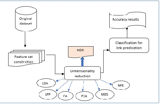
In this section, the proposed HDR is employed to show the impact of its use on a high dimension graph data obtained from a series of simulation experiments using MATLAB Version R2015b. For a fair comparison, we select two datasets: i) DBLP, which contains data about co-authoring among authors who have published one common paper at least, ii) arXiv in this network between two authors of scientific papers from the astrophysics archive. In this comparison, nine features for each data point are selected in both datasets. Basically, these points are selected based on their usage and significance in several applications of link prediction [19], where the link prediction predicts the possibility of a relationship between two not interconnected vertices in a graph, for the prediction of future interactions (links) that could take place between the authors (vertices). As in Figure 1 there are steps
to implement this work. In the first step, we take a sample from the original dataset as a graph G and turn it into a dataset shaped by the pair of vertices. In the second step, the features of each selected pair of vertices are computed, where the features extracted are as follows:
1- Shortest path length; this feature is the smallest number of links forming a path between a pair of vertices.
2- Common neighbors: it is the number of neighbors mutual to both nodes. 3- Sum of neighbors; it is the union of neighbors of each vertex from a pair. 4- Average neighbor degree.
5- Adamic/Adar similarity is the sum of the secondary common neighbors with a smaller weight than the primary neighbors.
6- Preferential attachment product of the number of neighbors of both vertices. 7- Leicht-Holme-Newman Index
8- Katz measure, which is the sum of lengths of all paths existing between each pair of vertices. 9- Jaccard’s Coefficient, which is the ratio between the number of common neighbors and the
number of total neighbors of each vertex.
In the third step, six different linear dimension reduction methods and the proposed method were implemented. One of the ways to tackle the link prediction issue is based on the classification, where this paper evaluates the impacts of dimensionality reduction as a preprocessing stage to the classifier construction in link prediction applications. Therefore, in the fourth step, the classification phase was carried, this step applies K-nearest neighbors’ algorithm (K-NN) and Support Vector Machine algorithm (SVM) as the classification algorithms to the reduced data set to obtain the link prediction.
The latent variables of DBLP and arXiv dataset set to best values by cross-validation technique, divided the dataset to classify the task into various folds.
The accuracy performance of each linear dimensionality reduction method is presented in Table 1, which is separated into three dataset fields, dimensionality reduction strategies and classification algorithms define a cell that has two numbers. The first one is the average precision (%) of the
classification models that are applied to the corresponding dimensionality reduction approaches to the respective classification algorithms and dataset. The second one indicates the number of features that are used in this simulation.
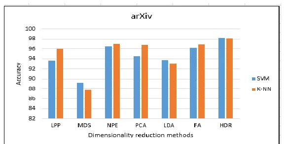
In the simulation experiments, the accuracy comparison is made of the suggested HDR approach with the PCA, NPE, LPP, MDS LDA, and FA methods. Figure 2 represents the results of DBLP dataset where firstly, the SVM classifier is utilized: it can be noticed that the classification outcome of the LPP algorithm is less robust than all of the existing algorithms with a smaller feature subset. As expected, the proposed HDR attained higher (89.22%) performance than any existing algorithms. The same experiment is repeated on DBLP dataset, where secondly, KNN is used as a classifier. It is observed that the NPE method was less accurate than others and achieved 84.77%, while the proposed HDR achieved higher accuracy, with 90.35%. With arXiv dataset where the SVM algorithm is applied, see Figure 3, the average precision was 93.69%, 89.17%, 96.5%, 94.45%, 93.72%, and 96.27% for LPP, MDS, NPE, PCA, LDA, and FA, respectively. The proposed method's accuracy was higher than all methods, where it reached about 98.22%. As shown in Figure 3, the arXiv dataset is
Da
tas
et
Alg
orit
hm
of
clas
sify
in
g Linear dimensionality reduction methods
LPP MDS NPE PCA LDA FA New method
DBLP
SVM 55.52 86.24 74.9 86.36 86.12 85.42 89.22
D 1 7 4 2 7 2 6
KNN 87.65 87.41 84.77 87.48 86.05 87.27 90.35
D 1 7 4 2 7 2 6
arXiv
SVM 93.69 89.17 96.5 94.45 93.72 96.27 98.22
D 1 1 3 2 2 4 7
KNN 95.97 87.73 96.97 96.83 93.09 96.91 98.14
D 1 1 3 2 2 4 7
repeated with K-NN algorithm, still, the HDR strategy outperformed all other methods, achieving 98.14%, with the less accurate MDS it at 87.73%.
6
Conclusion
In this paper, we proposed a new linear dimensionality reduction HDR method for the graph through a combination of NPE method which aims to preserve locality information and PCA method which preserves global information, based on finding common transformation matrix for both methods. The common transformation matrix was created based on formulating the generalized eigenvalue problem for two matrices then applied Rayleigh Quotient solution. The proposed method was compared with traditional linear dimensionality reduction methods to reduce the dimensionality of graph data to be used by the K nearest neighbor classifier (K-NN) and SVM algorithm. The latent variables of DBLP and arXiv dataset were set to best values by cross-validation approach and divided the dataset to classify the task into 10 dissimilar folds. The performances of all the methods were evaluated by using the performance accuracy metric. The results of our experiments on two graph
Figure 3: Comparison of dimensionality reduction methods accuracy by two different classification algorithms for arXiv dataset.
datasets showed that HDR outperforms other linear methods considered as popular in graph dimensionality reduction. This shows that the HDR algorithm based on combing PCA-and-NPE is an efficient approach for this area.
References
[1] J.P. Cunningham, Z. Ghahramani, Linear dimensionality reduction: Survey, insights, and generalizations, Journal of Machine Learning Research 16 (2015) 2859-2900.
[2] M. Vlachos, C. Domeniconi, D. Gunopulos, G. Kollios, N. Koudas, Non-linear dimensionality reduction techniques for classification and visualization, Proceedings of the eighth ACM SIGKDD international conference on Knowledge discovery and data mining, ACM, 2002, pp. 645-651.
[3] A. Barnawi, O. Batarfi, R. Elshawi, A. Fayoumi, R. Nouri, S. Sakr, On characterizing the performance of distributed graph computation platforms, Technology Conference on Performance Evaluation and Benchmarking, Springer, 2014, pp. 29-43.
[4] S. Sakr, E. Pardede, Graph data management: techniques and applications, Information Science Reference-Imprint of: IGI Publishing2011.
[5] O. Batarfi, R. El Shawi, A.G. Fayoumi, R. Nouri, A. Barnawi, S. Sakr, Large scale graph processing systems: survey and an experimental evaluation, Cluster Computing 18(3) (2015) 1189-1213.
[6] A. Tsymbal, S. Puuronen, M. Pechenizkiy, M. Baumgarten, D.W. Patterson, Eigenvector-Based Feature Extraction for Classification, FLAIRS Conference, 2002, pp. 354-358.
[7] M. Pechenizkiy, A. Tsymbal, S. Puuronen, On combining principal components with Fisher's linear discriminants for supervised learning, Foundations of Computing and Decision Sciences 31(1) (2006) 59-74.
[8] L. Tang, S. Peng, Y. Bi, P. Shan, X. Hu, A new method combining LDA and PLS for dimension reduction, PloS one 9(5) (2014) e96944.
[9] C. Chen, R. Bie, P. Guo, Combining LPP with PCA for microarray data clustering, Evolutionary Computation, 2008. CEC 2008.(IEEE World Congress on Computational Intelligence). IEEE Congress on, IEEE, 2008, pp. 2081-2086.
[10] X. Jiang, Asymmetric principal component and discriminant analyses for pattern classification, IEEE Transactions on Pattern Analysis & Machine Intelligence (5) (2008) 931-937.
[11] K.-C. Kwak, W. Pedrycz, Face recognition using an enhanced independent component analysis approach, IEEE Transactions on Neural Networks 18(2) (2007) 530-541.
[12] S. Moon, H. Qi, Hybrid dimensionality reduction method based on support vector machine and independent component analysis, IEEE transactions on neural networks and learning systems 23(5) (2012) 749-761.
[13] P. Yadhav, Adaptive firefly optimization on reducing high dimensional weighted word affinity graph, Compusoft 3(12) (2014) 1407.
[14] C.O.S. Sorzano, J. Vargas, A.P. Montano, A survey of dimensionality reduction techniques, arXiv preprint arXiv:1403.2877 (2014).
[15] C. Ding, X. He, K-means clustering via principal component analysis, Proceedings of the twenty-first international conference on Machine learning, ACM, 2004, p. 29.
[16] G.H. Dunteman, Principal components analysis, Sage1989.
[17] X. He, D. Cai, S. Yan, H.-J. Zhang, Neighborhood preserving embedding, Computer Vision, 2005. ICCV 2005. Tenth IEEE International Conference on, IEEE, 2005, pp. 1208-1213.
[18] M. Bao, Analysis and design principles of MEMS devices, Elsevier2005.