A Hybrid Approach for Software Development Effort Estimation using Neural networks, Genetic Algorithm, Multiple Linear Regression and Imperialist Competitive Algorithm

(1)

Int. J. Nonlinear Anal. Appl. 11 (2020) No. 1, 207-224 ISSN: 2008-6822 (electronic)

http://dx.doi.org/10.22075/ijnaa.2020.4259

A Hybrid Approach for Software Development Effort

Estimation using Neural networks, Genetic

Algorithm, Multiple Linear Regression and

Imperialist Competitive Algorithm

Mahdi Khazaiepoora_{*, Amid Khatibi Bardsiri}b_{, Farshid Keynia}c

a _{Computer engineering department, Kerman branch, Islamic Azad University, Kerman, Iran;} b _{Computer engineering department, Bardsir branch, Islamic Azad University, Bardsir, Iran;}

c _{Department of Energy Management and Optimization, Institute of Science and High Technology and Environmental}

Sciences, Graduate University of Advanced Technology, Kerman, Iran;

(Communicated by Madjid Eshaghi Gordji )

Abstract

Nowadays, effort estimation in software development is of great value and significance in project management. Accurate and appropriate cost estimation not only helps customers trust to invest but also has a significant role in logical decision making during project management. Different models of cost estimation are presented and employed to the date, but the models are application specific. In this paper, a three-phase hybrid approach is proposed to overcome the problem. In the first phase, features are selected using a combination of genetic algorithm and the perceptron neural network. In the second phase, impact factors are associated to each selected feature using multiple linear regression methods which act as coefficients of influence for each feature. In the last and the third phase, the feature weights are optimized by Imperialist Competitive Algorithm. To compare the proposed model for effort estimation with state-of-the-art models, three datasets are chosen as benchmark, namely COCOMO, Maxwell and Albrecht. The datasets are standard and publicly available for assessment. The experiments show promising results and average performance is improved by the proposed model for MMRE performance criterion on the datasets by 23%, 38% and 35%, respectively.

∗_{Mahdi Khazaiepoor}

Email address: [email protected], [email protected], [email protected](Mahdi

Khazaiepoora_{*, Amid Khatibi Bardsiri}b_{, Farshid Keynia}c₎

(2)

208 Khazaiepoor, Khatibi Bardsiri, Keynia

Keywords: Software Development Effort Estimation, Multiple Linear Regression (MLR), Neural Network, Genetic Algorithm (GA), Imperialist Competitive Algorithm (ICA), Maxwell, Albrecht, COCOMO.

2010 MSC: 68T99,68T20,68T05,68T10

1. INTRODUCTION

There is usually less chance in controlling, monitoring and programming as planned and predicted in software projects. Therefore, effort estimation is one of the most significant tasks in managing a software project. Efficient management of software projects need an accurate estimation [1]. Since, none of the estimation models is able to estimate the cost of a project accurately, no model is completely trustable in estimation process.

In recent years, researchers have provided lots of models for effort estimation of software development which can be divided into two groups of algorithmic and non-algorithmic. Algorithmic methods are mostly established based on mathematic methods which try to calculate the relation between project factors and development effort based on the mathematics contractions. Regression models such as Multi Linear Regression (MLR), Step Wise Regression (SWR) [2], Regression tree [3] and Software Living Management (SLIM) [4], Constructive Cost Model (COCOMO) [5] and Software Evaluation and Estimation of Resources – Software Estimating Model (SEER-SEM) [6] are some of the well-known algorithmic methods in effort estimation.

Non-algorithmic methods are based on active analysis of factors of software project. Some of the most practical methods are Learning Oriented Models (LOM), Analogy Based Estimation (ABE), and Expert Judgement (EJ). Researchers mostly tend to apply ABC model because it is more simple and practical [7, 8]. The method works based on data comparison of previous projects which are similar to present one. One of the problems of ABE model is that it does not provide a proper estimation for complex and incompatible data collections [9]; The method is unable to cover a vast area of software projects [10].

Some features of a software project make effort estimation process more difficult than they seem to be [11]. Some researches also claim that the constructed models are not necessarily practical for all data collections [12, 13]. Model combination, feature weighting and model weighting are some of the methods which have been more used recently [14].

Lots of methods are provided for effort estimation of software development but unfortunately most of them are not very practical in reality. One of the other challenges is the dependency of the approaches to data collections. In this paper, methods of algorithmic and non-algorithmic are approaches are combined to provide a novel model for effort estimation of software development which is highly practical for real-world scenarios.

Proposed method is explained in three phases. In the first phase, most influential features on de-velopment effort of software projects are selected by using both genetic algorithm and MLP neural network. In the second phase, impact factor of features are determined using MLR method with respect to the effect of each feature on project effort. In the final phase, the feature weights are optimized.

(3)

A Hybrid Approach for Software Development Effort Estimation... 11 (2020) No. 1, 207-224 209

2. RELATED WORKS

Soft computing techniques presented since 1994 [15] such as genetic algorithms and swarm intelli-gence are also applicable in the domain of software development effort estimation. Models of effort estimation in software projects such as COCOMO and genetic algorithm are presented in [16]. The models are tested in NASA software projects. Daldao et al. [17] performed experiments by leveraging Genetic programing (GP) and Neuro Programing (NP) and linear regression on problem solving of estimation of software projects. Sheta et al. [18] also investigated soft computing for effort estima-tion.

By literature review, one could deduce that combination of different strategies leads to better results [19]. Differences in the simplicity and flexibility of methods convince researchers to combine methods to cover higher range of solutions. For example, combination of analogy based methods with genetic algorithms [20] are some of the examples. Another example is the combination model of analogy and genetics to optimally tune the weighting parameters. Recently, the idea of clustering software projects gets attracts a lot of attention. Menzies et al. [21] conducted experiments in which results showed that localized models are preferred to global models. They also showed that not all global models achieve acceptable results in localized data even though achieved acceptable results on global data.

Battenberg [22] conducted experiments on regression-based estimation in two modes: (1) whole learning data at once and (2) clustered learning data. The results proves that the model improves by clustering learning data. Partitioned models on estimation of software development effort, are the models that estimates locally [23]. It is recommended to use clustering algorithms in order to divide the software project into groups and then an equation based regression is computed for each group as the estimated model.

ABE model is one of the well-known models in the effort estimation which is widely used in hybrid models. The combination of ABE with genetic algorithms [24], ABE with particle swarm optimization algorithm [25] And Artificial Neural Network (ANN) are some examples of combinations. Though hybrid models have a fairly acceptable accuracy based on ABE but the flexibility and versatility of the models is acceptable which can cover a wide range of software projects.

There are also new trends in software effort estimation. Ghatasheh et al. [26] also investigated the efficiency of applying the Firefly Algorithm as a metaheuristic optimization technique to optimize the parameters of different effort estimation models. These models are three variations of the Con-structive Cost Model COCOMO. Firouzian et al. [27] proposed a modular time and cost estimation algorithm on business processes which is applicable to development processes. Tianpei et al. [28] introduced a hyperparameter optimization architecture called OIL (Optimized Inductive Learning. They recommend using regression trees (CART) tuned by either different evolution or FLASH (a sequential model optimizer). They claim that this particular combination of learner and optimizers achieves superior results in a few minutes. Dhiraj et al. [29] stated that nowadays softwares are more data-centric and thus database has become such a crucial part of the software product, therefore to get more accurate estimations, the back-end part of web based application has to be taken into con-sideration. Fig. 1 shows a classification for the models presented to estimate the effort of software projects.

3. THE REQUIREMENTS OF THE PROPOSED METHOD

(4)

Figure 1: Classification of software effort estimation models

with cross validation method (leave-one-out) assign an impact factor to each selected feature. In the last phase, the coefficients are optimized using ICA.

3.1. Artificial Neural Network

The neural network model is a computer system which is simulated from the process of learning human brain. The application of neural networks in effort estimation started in 1993 and has yielded promising results. The benefits of neural networks in estimating costs are as following:

1. Eliminating the costly task of function discovery which take effort estimation variables as inputs and outputs the effort amount.

2. Eliminating the need to explicitly determine the mathematical estimation function before train-ing.

3. Independency of the number of cost variables.

The problem of too many parameter settings in neural networks could be considered as a disadvan-tage. Neural network applied in this paper is a two perceptron network. The number of neurons in the hidden layer is computed by trial and error. In the neural network, the number of entries is equal to the number of properties of the data set.

3.2. Genetic Algorithms

(5)

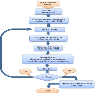
Figure 2: Flowchart of Genetic Algorithm (GA)

In each repetition of genetic algorithm, two operators of ”intersection” and ”mutation” are performed. The intersection operator is based on percentages with one population (usually 80%), and in the form of a mutation operator, a small percentage (usually 3%) of the population of each generation. The result of each of these operations is the production of a new member of the population. At the end of each repetition to select the number of members, the ”Select” operator selects a certain number of answers for the next generation. The steps in this algorithm are in accordance with the flowchart of Fig. 2.

3.3. Imperialist competitive algorithm

The imperialist competitive algorithm was introduced in 2007 by Dr. Atashpaz and professor Lucas [31]. This algorithm inspired by the same colonial phenomenon and colony in the real world which is based on the assumption that there are randomly created entities as the name of the countries and the countries are ranked according to a series of benchmarks.

The algorithm consists of two general phases:

1. Competition within an Empire. 2. Rivalry between empires.

(6)

Figure 3: Flowchart of Imperialist Competitive Algorithm (ICA)

4. PROPOSED MODEL

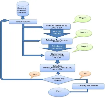
In this section, the proposed model is described in details. The main focus of the proposed model is on tuning parameters and weights as in all combinational models. Here, the proposed model consists of three phases:

1. Feature Selection:

In this section, the most effective features in the project effort are first selected using Genetic Algorithm and MLP Neural Network for each data set.

2. Impact Factor Computation:

In this step, impact factor is computed for each selected feature using multiple linear regression (MLR). The impact fact represents the coefficient of influence for each feature.

3. Weight Optimization:

At this stage, feature weights are optimized using the Imperialist competitive algorithm, known as ICA, considering the associated impact factor.

(7)

Figure 4: Flowchart of the proposed method

4.1. First Phase: Feature Selection

In this phase, a dataset is given as an input to genetic algorithm. Cost function in genetic algorithm is called Feature Selection Cost (FSC). Chromosome length is determined by the number of features in the dataset. Therefore, initial population is created randomly after determination of chromosome length. Each chromosome contains a chain of ‘1’s and ‘0’s, which means ‘chosen’ or ‘not chosen’ parallel features. Once the initial population is created, each member of population is evaluated by FSC function. Parameters of the neural network are then set and the function evaluates neural network with function ‘FITNN’ in the toolbox for five times with the mean score of five performance measures will return to genetic algorithm as cost response. The main loop of genetic algorithm begins after creation and evaluation of the initial population. The loop is repeated for 100 iteration and contain following steps:

1. Crossover: Crossover is an operation by which child chromosomes are created from selected parent chromosomes using Roulette wheel selection function. Three crossover types including single point, double point and uniform are applied by the chance of 0.2, 0.3, 0.5, respectively.

2. Response assessment: Once answers are produced from cross product, the answers are assessed by FSC function.

3. Mutation: Some responses are selected to be modified by mutation.

(8)

Figure 5: Flowchart of feature selection

5. Merging the three groups of population (initial population, population produced by crossover and population produced by mutation), collocating and selecting the best as the next generation population.

Since the best feature values are transferred to the next generation, the algorithm eventually outputs the best answer. Fig. 5 is showing the procedure of feature selection.

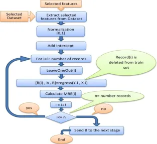
4.2. Second Phase: Impact Factor Computation

Once selected features of the dataset are extracted according to the feature extraction phase, features are normalized one by one according to equation (4.1).

xi0 =

xmax−xi

xmax−xmin

(4.1)

(9)

Figure 6: Flowchart of impact factor computation

Therefore, the impact factors associated to features using MLR method and the LEAVE-ONE-OUT technique are sent in a format of an array to the next phase. Fig. 6 shows the flowchart of impact factor computation.

4.3. Third Phase: Weight Optimization

In the previous phase, the impact factors are computed by MLR method in each step of the LEAVE-ONE-OUT technique. They are stored in an array and sent as input to the ICA algorithm. In this phase, ICA algorithm takes members of the array as initial population and starts optimizing the answers. Since the performance measures of the proposed methods are MDMRE, MMRE and PRED (0.25), the objective function in the ICA algorithm is to optimize the criteria. The constraint for MMRE and MDMRE measure is the smallest value and the constraint for PRED (0.25) measure is the highest value. Therefore, the objective function in the algorithm is to minimize the equation (4.2).

Z =|(P RED−(M M RE+M dM RE)| (4.2)

The output of this phase is a set of optimized weights. Fig. 7 shows the steps involved in this phase.

5. EVALUATION SETTINGS

(10)

Figure 7: Flowchart of weight optimization

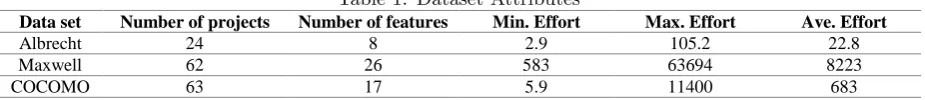
Table 1: Dataset Attributes

on software development projects are collected by researchers. Software application estimation data is employed for method analysis and model estimation. In recent years, researchers have employed various software development datasets. Three datasets are used to evaluate the proposed model. The name and general characteristics of the datasets are presented in Table 1.

Table (1): Dataset Attributes

Ave. Effort Max. Effort

Min. Effort Number of features

Number of projects Data set

22.8 105.2

2.9 8

24 Albrecht

8223 63694

583 26

62 Maxwell

683 11400

5.9 17

63 COCOMO

5.1.2 Performance metrics

Various parameters of performance measures are applied in different environments. The goal of most of the criteria is to measure the accuracy of estimation model, for example, the RE parameter shows the relative error which is the difference between the predicted value of the model and the actual value. The parameter is computed according to equation (3).

𝑅𝐸 = | 𝐸𝑠𝑡𝑖𝑚𝑎𝑡𝑒𝑑 − 𝐴𝑐𝑡𝑢𝑎𝑙 | (3)

“Estimated” is the predicted value by the proposed model and “Actual” is the actual value recorded in the dataset. The criterion of relative error is normalized and used according to equation (4).

𝑀𝑅𝐸𝑖 =

| 𝐸𝑠𝑡𝑖𝑚𝑎𝑡𝑒𝑑𝑖−𝐴𝑐𝑡𝑢𝑎𝑙𝑖 |

𝐴𝑐𝑡𝑢𝑎𝑙𝑖 (4)

Performance criteria are employed to assess the accuracy of estimations. In this paper, three performance criteria MDMRE, MMRE and PRED (0.25) are defined in equation (5, 6, 7).

𝑀𝑀𝑅𝐸 = 𝑚𝑒𝑎𝑛(𝑀𝑅𝐸) (5)

MdMRE = median(MRE) (6)

𝑃𝑅𝐸𝐷(0.25) =𝐴

𝑁 (7)

where A is the number of observations for which MRE are less than %25 and N is the total number of observations.

5.1. Datasets

Leveraging past observations in software projects is inevitable. To this end, a number of datasets on software development projects are collected by researchers. Software application estimation data is employed for method analysis and model estimation. In recent years, researchers have employed various software development datasets. Three datasets are used to evaluate the proposed model. The name and general characteristics of the datasets are presented in Table 1.

5.2. Performance metrics

Various parameters of performance measures are applied in different environments. The goal of most of the criteria is to measure the accuracy of estimation model, for example, the RE parameter shows the relative error which is the difference between the predicted value of the model and the actual value. The parameter is computed according to equation (5.1).

RE=| Estimated−Actual | (5.1)

“Estimated” is the predicted value by the proposed model and “Actual” is the actual value recorded in the dataset. The criterion of relative error is normalized and used according to equation (5.2).

M REi =

| Estimatedi −Actuali |

Actuali

(11)

Table 2: The initial settings and the values of parameters of genetic algorithms 5.1.3 Evaluation method

One of the evaluation methods is the cross validation method. In this method, the datasets are divided into k equal parts, and one of these k divisions is used as test data and K-1 other divisions are used as training data. The smaller the size of divisions, the more computations needed. Normally, the value of K can be equal to the number of dataset records. In our case, the method is the intersection validation method, known as leave-one-out method. Leave-One-Out method is used to evaluate the performance of the proposed model. For each execution, a record of dataset is considered as test data and the remaining data as training data. The action is repeated to the number of records to ensure each data is used once as test data. In each execution, MRE values for the test data is computed and in the end, MMRE values and PRED (0.25) for the test data is computed.

5.1.4 Initial settings

In this paper, Genetic Algorithm and MLP Neural Network for feature selection. Multiple linear regression (MLR) is used for impact factor computation for selected features. Finally, Imperialist Competitive Algorithm (ICA) is used to optimize feature weights. The initial settings and the values of parameters of genetic algorithms and ICA are obtained by trial and error method, as stated in Table 2 and Table 3.

Table (2): The initial settings and the values of parameters of genetic algorithms

Description Value

Name

Maximum of iteration 100

MaxIt

Num of initial population 30 Npop Crossover Percentage 0.8 Pc Mutation Percentage 0.3 Pm Mutation Rate 0.1 Mu

Tab (3): The initial settings and the values of parameters of ICA

Discription value

Name

MaxIt

Size of initial population Num of dataset records

Npop

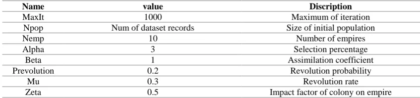
Number of empires 10 Nemp Selection percentage 3 Alpha Assimilation coefficient 1 Beta Revolution probability 0.2 Prevolution Revolution rate 0.3 Mu

Impact factor of colony on empire 0.5

Zeta

The structure of the neural network is a two-layer MLP, in which the number of neurons in the first layer is dependent to the dataset and is determined by trial and error. The first layer entries are the values of the selected attributes of each dataset. Therefore, the number of neural network inputs varies for each dataset. To train the neural network, LM (levemberg-Marquardt)

Table 3: The initial settings and the values of parameters of ICA 5.1.3 Evaluation method

5.1.4 Initial settings

Table (2): The initial settings and the values of parameters of genetic algorithms

Description Value

Name

MaxIt

Num of initial population 30 Npop Crossover Percentage 0.8 Pc Mutation Percentage 0.3 Pm Mutation Rate 0.1 Mu

Tab (3): The initial settings and the values of parameters of ICA

Discription value

Name

MaxIt

Size of initial population Num of dataset records

Npop

Number of empires 10 Nemp Selection percentage 3 Alpha Assimilation coefficient 1 Beta Revolution probability 0.2 Prevolution Revolution rate 0.3 Mu

Impact factor of colony on empire 0.5

Zeta

The structure of the neural network is a two-layer MLP, in which the number of neurons in the first layer is dependent to the dataset and is determined by trial and error. The first layer entries are the values of the selected attributes of each dataset. Therefore, the number of neural network inputs varies for each dataset. To train the neural network, LM (levemberg-Marquardt)

Performance criteria are employed to assess the accuracy of estimations. In this paper, three perfor-mance criteria MDMRE, MMRE and PRED (0.25) are defined in equation (5.3, 5.4, 5.5).

M M RE =mean(M RE) (5.3)

MdMRE = median (MRE) (5.4)

P RED(0.25) = A

N (5.5)

where A is the number of observations for which MRE are less than %25 and N is the total number of observations.

5.3. Evaluation method

5.4. Initial settings

(12)

Figure 8: a schematic presentation of the two layer neural network

Table 4: Results of effort estimation on COCOMO dataset

propagation function has been used. Training data, test data and validation data are divided by 70, 13 and 13 percent, respectively. Fig. 8 present the structure of the neural network.

Fig (8): a schematic of the two layer neural network

5.2 Experimental results

In this section, the results are compared against the results of other common models of effort estimation in order to validate the proposed model. The benchmark models are the RTM model [30], MLFE [31], LSE [32], OABE [33], CBR [34], and GA [35].

5.2.1 Results on the COCOMO Dataset

The COCOMO dataset is commonly used in the process of evaluating software appraisal model estimation models. The dataset contains data on software projects, including 62 projects with 17 features [5]. Table 4 shows the estimated effort by each of the models.

Table (4): Results of effort estimation on COCOMO dataset

Method Mmre MdMre Pred(0.25)

OABE 0.5 0.48 0.3

LSE 0.66 0.38 0.22

MLFE 1.48 0.72 0.14

RTM 0.54 0.47 0.25

GA 1.59 0.81 0.14

CBR k=3 0.58 0.48 0.27

CBR k=1 0.67 0.65 0.19

Proposed 0.52 0.54 0.3

As it is shown in Table 4, OABE model achieves the best result on MMRE criterion with a value of 0.30 and GA model achieves the worst result with a value of 1.39. The proposed model

are the values of the selected attributes of each dataset. Therefore, the number of neural network inputs varies for each dataset. To train the neural network, LM (levemberg-Marquardt) propagation function has been used. Training data, test data and validation data are divided by 70, 13 and 13 percent, respectively. Fig. 8 present the structure of the neural network.

6. EXPERIMENTAL RESULTS

In this section, the results are compared against the results of other common models of effort esti-mation in order to validate the proposed model. The benchmark models are the RTM model [34], MLFE [35], LSE [36], OABE [37], CBR [38], and GA [39].

6.1. COCOMO Dataset

The COCOMO dataset is commonly used in the process of evaluating software appraisal model estimation models. The dataset contains data on software projects, including 62 projects with 17 features [5]. Table 4 shows the estimated effort by each of the models.

(13)

achieves the second best result on MMRE criterion with a value of 0.58. For MdMRE criterion, the lowest value is achieved by LSE model with the value of 0.38 and the highest value is achieved by GA model with a value of 0.81. The proposed model is ranked fifth on MdMRE criterion with a value of 0.54. The results show that the proposed model on COCOMO dataset does not yield acceptable results. Fig. 9 shows a comparative diagram on the results.

Fig (9): results on COCOMO dataset for the three criteria: MMRE, MdMRE, and Pred(0.25)

5.2.2 Maxwell Dataset

One of the well-known and most widely used datasets for effort estimation is Maxwell dataset. The dataset includes 63 projects with 36 features [36]. Many researchers have used the dataset to evaluate the performance of their proposed model. Table 5 shows the results of effort estimation by different models on Maxwell dataset.

Tab (5): Results of effort estimation on Maxwell dataset

OABE 0.42 0.44 0.34

LSE 0.71 0.48 0.27

MLFE 0.71 0.48 0.27

RTM 0.46 0.41 0.32

GA 1.17 0.6 0.18

CBR K=2 0.51 0.39 0.39

CBR K=3 0.47 0.38 0.36

CBR K=5 0.44 0.36 0.32

Proposed 0.35 0.22 0.58

0 0.2 0.4 0.6 0.8 1 1.2 1.4 1.6 1.8

OABE LSE MLFE RTM GA CBR k=3 CBR k=1 Proposed

Mmre MdMre

Pred(0.25)

Figure 9: results on COCOMO dataset for the three criteria: MMRE, MdMRE, and PRED

6.2. Maxwell Dataset

Table 5: Results of effort estimation on Maxwell dataset

achieves the second best result on MMRE criterion with a value of 0.58. For MdMRE criterion, the lowest value is achieved by LSE model with the value of 0.38 and the highest value is achieved by GA model with a value of 0.81. The proposed model is ranked fifth on MdMRE criterion with a value of 0.54. The results show that the proposed model on COCOMO dataset does not yield acceptable results. Fig. 9 shows a comparative diagram on the results.

Fig (9): results on COCOMO dataset for the three criteria: MMRE, MdMRE, and Pred(0.25)

5.2.2 Maxwell Dataset

Tab (5): Results of effort estimation on Maxwell dataset

OABE 0.42 0.44 0.34

LSE 0.71 0.48 0.27

MLFE 0.71 0.48 0.27

RTM 0.46 0.41 0.32

GA 1.17 0.6 0.18

CBR K=2 0.51 0.39 0.39

CBR K=3 0.47 0.38 0.36

CBR K=5 0.44 0.36 0.32

Proposed 0.35 0.22 0.58

0 0.5 1 1.5 2

OABE LSE MLFE RTM GA CBR k=3 CBR k=1 Proposed

Chart Title

Mmre

MdMre Pred(0.25)

According to Table 5, the best value for the MMRE parameter is 0.35 and is related to the proposed model, and the worst value for this parameter is equal 0.71 which is related to the MLFE and LSE models.

For the MdMER parameter, the best value is 0.22, which is commonly related to the proposed model. The worst value is 0.60, which is related to the GA model.

(14)

According to Table (5), the best value for the MMRE parameter is 0.35 and is related to the proposed model, and the worst value for this parameter is equal 0.71 which is related to the MLFE and LSE models.

For the MdMER parameter, the best value is 0.22, which is commonly related to the proposed model. The worst value is 0.60, which is related to the GA model.

Finally, the best value for the PRED(0.25) parameter is equal to 0.58 Which is related to the proposed model and The worst value for this parameter is related to the GA model and to 0.18. The results show that the proposed model has worked very well on this data set, and the accuracy achieved is desirable. Diagram (10) depicts these results.

 Fig (10): MMRE, MdMRE, and Pred(0.25) results on Maxwell dataset

5.2.3 Albrecht Dataset

Albrecht dataset contains information on 24 projects and has 8 features which are used in the estimation process [37]. Although the number of projects in this data set is low but has been used by many researchers to estimate the effort to evaluate the models. We also use this dataset to evaluate our proposed model. The results of various models on this dataset are presented for the three parameters MdMRE, MMRE and PRED (0.25) shown in Table (6).

Tab (6): the estimated effort by each of the models on Albrecht

0 0.2 0.4 0.6 0.8 1 1.2 1.4

OABE LSE MLFE RTM GA CBR K=2 CBR K=3 CBR K=5 Proposed

Mmre

MdMre

Pred(0.25)

Figure 10: Results on COCOMO dataset for the three criteria: MMRE, MdMRE, and PRED

Table 6: Results of effort estimation on Albrecht dataset Method Mmre MdMre Pred (0.25)

OABE 0.4 0.37 0.45

LSE 0.63 0.30 0.37

MLFE 0.65 0.30 0.37

RTM 0.61 0.40 0.33 GA 0.45 0.38 0.33

CBR+FA 0.38 0.29 0.48

CBR+PSO 0.52 0.24 0.57

Proposed 0.34 0.18 0.58

As it is shown in Table 6, the proposed model achieves the best results on MMRE criterion with a value of 0.34 and MLFE model achieves the worst results on MMRE criterion with a value of 0.65. The proposed model also achieves the best results on MdMRE criterion with a value of 0.18 and RTM model achieves the worst results on MdMRE criterion with a value of 0.4. Finally, the best results on PRED (0.25) criterion is achieved by proposed model with a value of 0.57. The worst results with a value of 0.33, which is achieved by RTM and GA models. The results show that the proposed model also has an acceptable performance on Albrecht dataset. Fig. 11 shows these results in a diagram.

Fig (11): MMRE, MdMRE, and Pred(0.25) results on Albrecht dataset

6. RESULTS

The results show that the proposed model failed to perform well on the COCOMO dataset for the criterion MdMRE. The reason for this is the limited variety of projects in this data set In the Maxwell dataset, according to the results, the proposed model in each of the parameters of the MdMRE, MMRE and PRED ranked first. Therefore, it provides an acceptable performance on this data set. Albrecht dataset is a relatively standard dataset, which can lead to an improved

0 0.1 0.2 0.3 0.4 0.5 0.6 0.7

OABE LSE MLFE RTM GA CBR+FA CBR+PSO Proposed

Mmre MdMre Pred(0.25)

6.3. Albrecht Dataset

Albrecht dataset contains information on 24 projects and has 8 features which are used in the estimation process [41]. Although the number of projects in this data set is low but has been used by many researchers to estimate the effort to evaluate the models. We also use this dataset to evaluate our proposed model. The results of various models on this dataset are presented for the three parameters MdMRE, MMRE and PRED (0.25) shown in Table 6.

6.4. Analysis of results

(15)

Method Mmre MdMre Pred (0.25)

OABE 0.4 0.37 0.45

LSE 0.63 0.30 0.37

MLFE 0.65 0.30 0.37

RTM 0.61 0.40 0.33 GA 0.45 0.38 0.33

CBR+FA 0.38 0.29 0.48

CBR+PSO 0.52 0.24 0.57

Proposed 0.34 0.18 0.58

Fig (11): MMRE, MdMRE, and Pred(0.25) results on Albrecht dataset

6. RESULTS

The results show that the proposed model failed to perform well on the COCOMO dataset for the criterion MdMRE. The reason for this is the limited variety of projects in this data set In the Maxwell dataset, according to the results, the proposed model in each of the parameters of the MdMRE, MMRE and PRED ranked first. Therefore, it provides an acceptable performance on this data set. Albrecht dataset is a relatively standard dataset, which can lead to an improved

0 0.1 0.2 0.3 0.4 0.5 0.6 0.7

OABE LSE MLFE RTM GA CBR+FA CBR+PSO Proposed

Mmre MdMre Pred(0.25)

Figure 11: Results on Albrecht dataset for the three criteria: MMRE, MdMRE, and PRED

Table 7: Analysis of Results

model accuracy. The results of the proposed model have improved dramatically on this data set. The most important one can be the proper weighting and the exact choice of the solution function despite the low number of projects in this dataset, the proposed model has been able to deliver satisfactory results. And this certainly depends on the quality of the projects in this dataset. Table 7 shows the average improvement performance of the suggested model in each of the data sets for each of the MdMRE, MMRE and (0.25) PRED models.

Tab (7): results analyzes

The average improvement in percentage

MMRE MdMRE PRED(0.25) Dataset % 36 % 4 % 32 COCOMO % 40 % 47 % 72 MaxWell % 35 %45 % 40 Albrecht

7.

CONCLUSION

The accurate estimation of the software development effort is crucial for software projects. The tendency of researchers in recent years and increasing trend of researches proves the necessity to provide an appropriate model of software development effort estimation. Although a wide range of models are presented to overcome the problem but the results shows that the models are application specific and heavily depends on the project type. The proposed method is presented in three phases; In the first phase, features are selected using a combination of genetic algorithm and the perceptron neural network. In the second phase, impact factors are associated to each selected feature using multiple linear regression methods and representing as coefficient of influence for each feature. In the last and the third phase, the feature weights are optimized by Imperialist Competitive Algorithm. Experimental results show that the proposed model achieves acceptable results on Maxwell and Albrecht datasets but for COCOMO dataset, the obtained results are relatively weaker. A disadvantage of the proposed model is the dependency to the dataset which is the same as other models. To evaluate the proposed model, MdMRE, MMRE and PRED (0.25) are used as performance criteria. Results show that the proposed model is more independent to the dataset than other models, because of the hybrid architecture. In the future, it is recommended to employ hybrid approach to overcome the problem with a combination of models.

REFERENCES

MdMRE, MMRE and PRED ranked first. Therefore, it provides an acceptable performance on this data set. Albrecht dataset is a relatively standard dataset, which can lead to an improved model accuracy. The results of the proposed model have improved dramatically on this data set. The most important one can be the proper weighting and the exact choice of the solution function despite the low number of projects in this dataset, the proposed model has been able to deliver satisfactory results. And this certainly depends on the quality of the projects in this dataset. Table 7 shows the average improvement performance of the suggested model in each of the data sets for each of the MdMRE, MMRE and PRED (0.25) models.

7. CONCLUSION

(16)

but for COCOMO dataset, the obtained results are relatively weaker. A disadvantage of the pro-posed model is the dependency to the dataset which is the same as other models. To evaluate the proposed model, MdMRE, MMRE and PRED (0.25) are used as performance criteria. Results show that the proposed model is more independent to the dataset than other models, because of the hybrid architecture. In the future, it is recommended to employ hybrid approach to overcome the problem with a combination of models.

References

[1] Jorgensen, M. and M. Shepperd, A systematic review of software development cost estimation studies. IEEE Transactions on software engineering, 2006. 33(1): p. 33-53.

[2] Costagliola, G., et al., Class point: an approach for the size estimation of object-oriented systems. IEEE Transactions on Software Engineering, 2005.31(1): p. 52-74.

[3] Breiman, L., et al., Classification and regression trees (cart) wadsworth. Pacific Grove, CA, 1984. [4] Putnam, L.H., A general empirical solution to the macro software sizing and estimating problem. IEEE transactions on Software Engineering, 1978(4): p. 345-361.

[5] Boehm, B.W., Software engineering economics. IEEE transactions on Software Engineering, 1984(1): p. 4-21.

[6] Jensen, R. An improved macrolevel software development resource estimation model. in 5th ISPA Conference. 1983.

[7] Bardsiri, V.K., et al., Increasing the accuracy of software development effort estimation using projects clustering. IET software, 2012. 6(6): p. 461-473.

[8] Kocaguneli, E., et al., Exploiting the essential assumptions of analogy-based effort estimation. IEEE transactions on software engineering, 2011. 38(2): p. 425-438.

[9] Huang, Y.-S., et al., Prototype optimization for nearest-neighbor classification. Pattern Recogni-tion, 2002. 35(6): p. 1237-1245.

[10] Bardsiri, V.K., et al., LMES: A localized multi-estimator model to estimate software develop-ment effort. Engineering Applications of Artificial Intelligence, 2013. 26(10): p. 2624-2640.

[11] Bardsiri, A.K. and S.M. Hashemi, Electronic services, the only way to realize the global village. International Journal of Mechatronics, Electrical and Computer Technology, 2013. 3(6): p. 1039-1041.

[12] ˇCeke, D. and B. Milaˇsinovi´c, Early effort estimation in web application development. Journal of Systems and Software, 2015. 103: p. 219-237.

[13] Khatibi, E. and V.K. Bardsiri, Model to estimate the software development effort based on in-depth analysis of project attributes. IET software, 2015. 9(4): p. 109-118.

[14] Wu, D., J. Li, and Y. Liang, Linear combination of multiple case-based reasoning with optimized weight for software effort estimation. The Journal of Supercomputing, 2013. 64(3): p. 898-918. [15] Zadeh, L.A., Soft computing and fuzzy logic, in Fuzzy Sets, Fuzzy Logic, and Fuzzy Systems: Selected Papers by Lotfi a Zadeh. 1996, World Scientific. p. 796-804.

[16] Sheta, A.F., Estimation of the COCOMO model parameters using genetic algorithms for NASA software projects. Journal of Computer Science, 2006. 2(2): p. 118-123.

[17] Dolado, J., LF andez,”Genetic programming, neural network and linear regression in software project estimation”. Proceedings of the INSPIRE III, Process Improvement through training and education: p. 157-171.

(17)

[19] Chiu, N.-H. and S.-J. Huang, The adjusted analogy-based software effort estimation based on similarity distances. Journal of Systems and Software, 2007. 80(4): p. 628-640.

[20] Song, Q. and M. Shepperd, Predicting software project effort: A grey relational analysis based method. Expert Systems with Applications, 2011. 38(6): p. 7302-7316.

[21] Menzies, T., et al. Local vs. global models for effort estimation and defect prediction. in 2011 26th IEEE/ACM International Conference on Automated Software Engineering (ASE 2011). 2011. IEEE.

[22] Bettenburg, N., M. Nagappan, and A.E. Hassan. Think locally, act globally: Improving defect and effort prediction models. in 2012 9th IEEE Working Conference on Mining Software Repositories (MSR). 2012. IEEE.

[23] Rodr´ıguez, D., et al. Segmentation of software engineering datasets using the m5 algorithm. in International Conference on Computational Science. 2006. Springer.

[24] Huang, S.-J. and N.-H. Chiu, Optimization of analogy weights by genetic algorithm for software effort estimation. Information and software technology, 2006. 48(11): p. 1034-1045.

[25] Bardsiri, V.K., et al., A PSO-based model to increase the accuracy of software development effort estimation. Software Quality Journal, 2013. 21(3): p. 501-526.

[26] Ghatasheh, N., et al., Optimizing software effort estimation models using firefly algorithm. arXiv preprint arXiv:1903.02079, 2019.

[27] Firouzian, I., M. Zahedi, and H. Hassanpour, Investigation of the Effect of Concept Drift on Data-Aware Remaining Time Prediction of Business Processes. International Journal of Nonlinear Analysis and Applications, 2019. 10(2): p. 153-166.

[28] Xia, T., et al., Hyperparameter optimization for effort estimation. arXiv preprint arXiv:1805.00336, 2018.

[29] Goswami, D.K., S. Chakrabarti, and S. Bilgaiyan, Effort Estimation of Web Based Applications Using ERD, Use Case Point Method and Machine Learning, in Automated Software Engineering: A Deep Learning-Based Approach. 2020, Springer. p. 19-37.

[30] Goldberg, D.E. and J. Richardson. Genetic algorithms with sharing for multimodal function optimization. in Genetic algorithms and their applications: Proceedings of the Second International Conference on Genetic Algorithms. 1987. Hillsdale, NJ: Lawrence Erlbaum.

[31] Atashpaz-Gargari, E. and C. Lucas. Imperialist competitive algorithm: an algorithm for opti-mization inspired by imperialistic competition. in 2007 IEEE congress on evolutionary computation. 2007. IEEE.

[32] Khatibi Bardsiri, A., S.M. Hashemi, and M. Razzazi, GVSEE: a new global model to estimate software services development effort. Journal of the Chinese Institute of Engineers, 2016. 39(6): p. 765-776.

[33] Keung, J., E. Kocaguneli, and T. Menzies, Finding conclusion stability for selecting the best effort predictor in software effort estimation. Automated Software Engineering, 2013. 20(4): p. 543-567.

[34] Jørgensen, M., U. Indahl, and D. Sjøberg, ”Software effort estimation by analogy and regression toward the mean”. Journal of Systems and Software, 2003. 68(3): p. 253-262.

[35] Mendes, E., N. Mosley, and S. Counsell. A replicated assessment of the use of adaptation rules to improve Web cost estimation. in 2003 International Symposium on Empirical Software Engineering, 2003. ISESE 2003. Proceedings. 2003. IEEE.

[36] Walkerden, F. and R. Jeffery, An empirical study of analogy-based software effort estimation. Empirical software engineering, 1999. 4(2): p. 135-158.

(18)

[38] Bisio, R. and F. Malabocchia. Cost estimation of software projects through case base reasoning. in International Conference on Case-Based Reasoning. 1995. Springer.

[39] Choudhary, K., GA based Optimization of Software Development effort estimation. IJCST, 2010. 1(1): p. 38-40.

[40] Maxwell, K. and K. Maxwell, Applied statistics for software managers. 2002: Prentice Hall PTR Englewood Cliffs.