HARDWARE SYSTEM
by
Fady Hussein
A dissertation
submitted in partial fulfillment
of the requirements for the degree of
Doctor of Philosophy in Electrical and Computer Engineering
Boise State University
DEFENSE COMMITTEE AND FINAL READING APPROVALS
of the dissertation submitted by
Fady Hussein
Dissertation Title: HexArray: A Novel Self-Reconfigurable Hardware System
Date of Final Oral Examination: 13 March 2017
The following individuals read and discussed the dissertation submitted by student Fady Hussein, and they evaluated his presentation and response to questions during the final oral examination. They found that the student passed the final oral examination.
I am using this opportunity to express my gratitude to everyone who supported me
throughout the course of this dissertation. I am thankful for their aspiring guidance,
invalu-ably constructive criticism and friendly advice during the project work, specifically my
advisor (Dr. Nader Rafla) and his research team, Luka Daoud and Shelton Jacinto.
Fady Hussein is a PhD Candidate at Electrical and Computer Engineering at Boise
State University. He joined the PhD program on August 2013. He received his MSc
degree from Louisiana State University and bachelors degree in Electrical Engineering
at Birzeit University, Palestine. Fady is, currently, a senior test engineer for DRAM at
Micron Technology in Boise, Idaho. His main research focuses on evolvable hardware
and reconfigurable computing. Currently, he is developing a framework for an evolvable
system that can be utilized in design automation, image processing, reverse engineering
and fault-tolerant systems.
Evolvable hardware (EHW) is a powerful autonomous system for adapting and finding
solutions within a changing environment. EHW consists of two main components: a
reconfigurable hardware core and an evolutionary algorithm. The majority of prior research
focuses on improving either the reconfigurable hardware or the evolutionary algorithm in
place, but not both. Thus, current implementations suffer from being application oriented
and having slow reconfiguration times, low efficiencies, and less routing flexibility. In this
work, a novel evolvable hardware platform is proposed that combines a novel
reconfig-urable hardware core and a novel evolutionary algorithm.
The proposed reconfigurable hardware core is a systolic array, which is called
HexAr-ray. HexArray was constructed using processing elements with a redesigned architecture,
called HexCells, which provide routing flexibility and support for hybrid
reconfigura-tion schemes. The improved evolureconfigura-tionary algorithm is a genome-aware genetic
algo-rithm (GAGA) that accelerates evolution. Guided by a fitness function the GAGA utilizes
context-aware genetic operators to evolve solutions. The operators are genome-aware
con-strained (GAC) selection, genome-aware mutation (GAM), and genome-aware crossover
(GAX). The GAC selection operator improves parallelism and reduces the redundant
eval-uations. The GAM operator restricts the mutation to the part of the genome that affects the
selected output. The GAX operator cascades, interleaves, or parallel-recombines genomes
at the cell level to generate better genomes. These operators improve evolution while not
limiting the algorithm from exploring all areas of a solution space.
The system was implemented on a SoC that includes a programmable logic (i.e.,
the GAGA. A computationally intensive application that evolves adaptive filters for image
processing was chosen as a case study and used to conduct a set of experiments to prove the
developed system robustness. Through an iterative process using the genetic operators and
a fitness function, the EHW system configures and adapts itself to evolve fitter solutions.
In a relatively short time (e.g., seconds), HexArray is able to evolve autonomously to the
desired filter.
By exploiting the routing flexibility in the HexArray architecture, the EHW has a
simple yet effective mechanism to detect and tolerate faulty cells, which improves
sys-tem reliability. Finally, a mechanism that accelerates the evolution process by hiding the
reconfiguration time in an “evolve-while-reconfigure” process is presented. In this process,
the GAGA utilizes the array routing flexibility to bypass cells that are being configured and
evaluates several genomes in parallel.
DEDICATION . . . iv
ACKNOWLEDGMENTS . . . v
AUTOBIOGRAPHICAL SKETCH . . . vi
ABSTRACT . . . vii
LIST OF TABLES . . . xiv
LIST OF FIGURES . . . xvi
LIST OF ABBREVIATIONS . . . xxv
LIST OF SYMBOLS . . . xxix
LIST OF LISTINGS . . . xxxii
LIST OF ALGORITHMS . . . xxxiii
1 Introduction . . . 1
1.1 Evolvable Hardware (EHW) . . . 3
1.2 Main Components of Evolvable Hardware . . . 4
1.2.1 Reconfigurable Hardware Core . . . 5
1.2.2 Evolutionary Algorithms (EAs) . . . 6
1.4 Motivation and Research Objectives . . . 11
1.5 Contributions . . . 12
1.6 Dissertation Overview . . . 13
2 Reconfigurable Hardware Core . . . 15
2.1 Introduction . . . 15
2.2 Properties of Reconfigurable Hardware Cores . . . 16
2.2.1 Architecture . . . 17
2.2.2 Interconnect . . . 17
2.2.3 Fabric Structure . . . 18
2.2.4 Reconfiguration Schemes . . . 18
2.3 Reconfigurable Architectures . . . 20
2.3.1 Commercial Simple Programmable Logic Devices . . . 20
2.3.2 Commercial High-Capacity Programmable Logic Devices . . . 25
2.3.3 Custom Architectures . . . 30
2.4 Summary . . . 38
3 Evolutionary Algorithms . . . 40
3.1 Introduction . . . 40
3.2 Genetic Operators . . . 40
3.2.1 Selection . . . 40
3.2.2 Mutation . . . 42
3.2.3 Crossover . . . 42
3.2.4 Elitism . . . 42
3.3 Fitness Functions . . . 43
3.5 Genetic Algorithm . . . 48
3.6 Summary . . . 50
4 Evolvable Hardware Systems . . . 52
4.1 Introduction . . . 52
4.2 Classifications of Evolvable Hardware Systems . . . 52
4.2.1 Hardware Platform . . . 53
4.2.2 Reconfiguration Scheme . . . 54
4.2.3 Evolutionary Algorithm . . . 54
4.2.4 Evolutionary Level of Abstraction . . . 54
4.2.5 Hardware Evolution Type . . . 55
4.2.6 Operation Mode . . . 55
4.2.7 Application Area . . . 56
4.3 Evolvable Hardware Implementations . . . 56
4.3.1 Systolic Arrays . . . 58
4.4 Summary . . . 61
5 HexArray Platform Design . . . 62
5.1 Introduction . . . 62
5.2 HexArray Simulator . . . 63
5.3 Proposed Reconfigurable Hardware Core . . . 66
5.3.1 A Novel Processing Element – HexCell . . . 66
5.3.2 A Novel Systolic Array – HexArray . . . 70
5.4 Proposed Genome-Aware Genetic Algorithm (GAGA) . . . 74
5.4.1 Algorithm Utility Functions . . . 75
5.4.3 Genome-Aware Mutation (GAM) . . . 86
5.4.4 Genome-Aware Crossover (GAX) . . . 86
5.4.5 Genome-Aware Pruner (GAP) . . . 91
5.5 Overall System Workflow . . . 92
5.6 Additional Features . . . 97
5.6.1 A Novel Fault Detection and Tolerance Mechanism . . . 97
5.6.2 A Novel Evolve-while-Reconfigure Mechanism . . . 99
5.7 HexArray Versus State-of-the-Art Systolic Array . . . 102
5.7.1 Degree of Polynomial . . . 102
5.8 Summary . . . 103
6 Evaluations and Implementation Analysis . . . 107
6.1 Introduction . . . 107
6.2 Evolution Speed Evaluations . . . 108
6.2.1 Experiment 1: HexArray Outperforms State-of-the-Art Systolic Array . . . 109
6.2.2 Experiment 2: GAC Selection Accelerates Evolution . . . 115
6.2.3 Experiment 3: GAM Outperforms Traditional Mutation . . . 118
6.2.4 Experiment 4: GAX Outperforms Traditional Crossover . . . 123
6.2.5 Experiment 5: The Effect of Population Size on Evolution . . . 127
6.2.6 Experiment 6: Adaptive Filter Evaluations . . . 131
6.2.7 Experiment 7: Autonomous Evolution for Variety of Filters . . . 138
6.3 Implementation Analysis . . . 152
6.3.1 Resource Utilization . . . 156
6.4 Summary . . . 160
7 Conclusion . . . 163
7.1 Future Work . . . 166
REFERENCES . . . 171
A Image Processing . . . 188
A.1 Introduction . . . 189
A.2 Image Groups: . . . 189
2.1 Comparison of VRC and DPR. . . 20
4.1 Summary of hardware evolution types. . . 55
5.1 Simulator parameters to control the evolution process. . . 65
5.2 Function set for the selected image processing application. . . 69
5.3 HexArray in comparison to Cartesian Array with RectCell. . . 102
6.1 A collection of image groups used in the experiments. . . 108
6.2 Summary of the best and median fitness values collected for evaluation of Cartesian arrays based on traditional RectCells and modified RectCells and HexArray. . . 112
6.3 Data were collected by running 100 iterations of 1000 genomes generated by unconstrained random selection in comparison to GAC random selection. 116 6.4 Median normalized fitnesses were collected by running 100 iterations of 10,000 genomes generated by traditional mutation in opposition to GAM with different numbers of mutation bits. . . 120
6.5 Best normalized fitnesses were collected by running 100 iterations of 10000 genomes generated by traditional mutation in opposition to GAM with different numbers of mutation bits. . . 121
6.6 Best and median fitnesses obtained from 100 runs of 8×8 HexArray with crossover and GAX running in three modes. . . 126
fixed total number of genomes. . . 128
6.8 Best and median fitnesses obtained from 50 runs of 8×8 HexArray with different generation/population combinations. . . 129
6.9 Variety of image groups to explore the autonomous adaptivity of the system. 140 6.10 Resource utilization reported by Vivado for 8×8 HexArray. . . 156
7.1 Function set for an OCR application. . . 169
A.1 Properties of 10% and 25% Salt and Pepper noise images. . . 189
A.2 Properties of EdgaDetect, Thresholding, and Gaussian image groups. . . 192
A.3 Properties of Lena image with different levels of impulsive noise. . . 192
A.4 Properties of Cameraman image with different levels of impulsive noise. . . 195
A.5 Properties of experiment 7 image groups. . . 197
1.1 Evolvable hardware and embryonic hardware are the main branches of
bio-inspired hardware. . . 2
1.2 EHW is the field where biology, electrical engineering, and computer sci-ence meet. . . 3
1.3 Main components of EHW. . . 4
1.4 Evolution cycle between (a) biology and (b) electronics [1]. . . 7
1.5 Intrinsic EHW types based on where the EA is running [2]. . . 10
2.1 Hardware core properties in terms of structure and reconfiguration. . . 16
2.2 VRC and DPR: the two reconfiguration schemes for EHW [3]. . . 18
2.3 Classifications of reconfigurable architectures. . . 21
2.4 Simplified SPLD, adapted from [4]. . . 22
2.5 PROM: the simplest programmable architecture [5]. . . 22
2.6 PLA has a programmable AND plane and a programmable OR plane. . . 23
2.7 PAL architecture with loopback wiring to improve flexibility [6]. . . 24
2.8 A simplified block diagram of CPLD architecture [4]. . . 25
2.9 MAX V: a CPLD manufactured by Altera [7]. . . 26
2.10 LABs are the building blocks of CPLDs. Each LAB has 10 LEs [7]. . . 27
2.11 Simplified FPGA block diagram [4]. . . 28
2.12 Two slices per CLB, Xilinx 7 series [8]. . . 29
architecture [8]. . . 30
2.14 Block diagram of MONTIUM tile [9]. . . 32
2.15 Reconfigurable architecture based on fuzzy logic, Fuzzy CoCo [10]. . . 33
2.16 Colt reconfigurable architecture with 16 functional units, smart crossbar interconnect and 6 data ports [11]. . . 34
2.17 Garp reconfigurable architecture [12]. . . 35
2.18 KressArray: a non-von-Neumann reconfigurable architecture [13]. . . 36
2.19 Pleiades: a heterogeneous coarse-grained reconfigurable platform [14]. . . . 37
2.20 POEtic: a reconfigurable bio-inspired architecture [15]. . . 38
3.1 A general workflow for evolutionary algorithms. The closer the fitness is to zero, the better the solution is. . . 41
3.2 GP represents genomes as parse trees. Tree nodes are mapped to computer programs. The shown tree is equivalent to the program MIN(In1+(In2 & 255), 10+(In3× In1)). . . 46
3.3 Example of two-bit multiplier circuit evolved using CGP by Miller et al. [16]. Each integer in the genotype defines a function selection or a routing option. Some chromosomes were left unused in this example. . . 47
4.1 Classification schemes of EHW. . . 53
4.2 Type R systolic array proposed Kung et al. in 1978 [17]. . . 59
4.3 Type H systolic array proposed Kung et al. in 1979 [18]. . . 59
4.4 A 5×5 systolic array of state-of-the-art PEs, where the array uses a single output and PEs use DPR reconfiguration scheme. . . 60
by algorithm with a 63% noise reduction. (c) Reference image used for the
fitness calculations. . . 64
5.2 The HexCell structure and representation: the HexCell’s functional unit is
on a dynamic partition while the remaining logic is static. The HexCell
chromosome has four genes, where three genes implicate a VRC and one
implicates a DPR. . . 66
5.3 Data window controller formats the input data stream received from the
DMA as a sliding data window accessible by the array input controllers,
which are controlled by thei GENOMEand fed into the array cells. . . 71
5.4 4×4 HexArray with AICs (shown in red) and AOCs (shown in yellow). . . . 73
5.5 Array output controller module which accumulates the absolute differance
between the evolved pixel and the reference pixel for “Expected Count”
pixels. . . 74
5.6 HexArray can have different levels of dependencies where (1) the static
chromosome-level dependency is unaware of the cells’ functional units
dependencies, (2) the dynamic chromosome-level dependency is aware of
the cells’ functional units dependencies, and (3) the dynamic gene-level
dependency is aware of the cells’ functional units dependencies and the
cells’ output ports selection. . . 78
5.7 Boundbox and free boundbox for a genome of HexArray. . . 79
5.8 The probability distribution for selecting a genome out of 20 parents.
Be-cause Genome 0 is the parent with the best fitness, it has the highest chance
(22.3%) of being selected. Genome 19 is the one with the worst fitness
(compared to others); thus, it has the lowest chance (2.5%). . . 84
puts. The darker the cell is, the lower the chance is for f to reach an output.
For example, the probability value of 0.5 was obtained from the probability
of f being routed through X or Y (0.25+0.25). . . 86
5.10 GAX modes. (Top) An offspring is generated by cascading genomes, where
one feeds into the other. (Middle) An offspring is generated by interleaving
genomes at the cell level. (Bottom) An offspring is generated by combining
genomes in parallel and inserting some cells in-between with randomly
selected functions. . . 88
5.11 HexArray platform with HexArray and GAGA. HexArray, array input
con-trollers, array output concon-trollers, data widow controller, and genome
regis-ter are implemented on the FPGA programmable logic, while the GAGA
is implemented on the processor. . . 94
5.12 Data propagation in HexArray, where a pixel is processed by PE1,1at time
1 and by PE8,8at time 19. . . 96
5.13 (a) Single-cell fault results in unexpected outputs. (b) Multi-cell fault
re-sults in unexpected outputs. (c) Example of an output dependency tree,
where any fault inPE1,1,PE1,2,PE2,1, andPE1,3will affect the output. . . 97
5.14 Example for fault detection mechanism using row by row testing where the
array output of a predefined genome is checked against a pre-calculated
output. If the outputs are matching, then the circuit is fault-free. If the
outputs are not matching, then the circuit has one or more faulty cells. A
row by row test is needed to determine which cells are faulty. . . 98
5.15 Flowchart for the proposed fault detection and tolerance mechanism. . . 100
while some of the cells are being programmed (shown in dark gray). . . 101
5.17 Degree of polynomial of HexArray is higher than Cartesian arrays. . . 103
5.18 Fitting the degree of polynomial of HexArray and state-of-the-art systolic
array. . . 104
6.1 (a) A Cartesian array constructed using classical RectCells. One output is
evaluated per genome (based onSelO), and a cell functional output is routed
to the E and S ports. (b) A Cartesian array constructed using “modified”
RectCells, where an output multiplexer has been added to every cell output
to select from the N port, W port or the functional unit output. (c) and (d)
are similar to (a) and (b), respectively, but with evaluating five outputs per
one genome. . . 110
6.2 Evolution is accelerated by the HexArray architecture in comparison to
Cartesian arrays with traditional RectCells and with modified RectCells.
Adding parallelism to the Cartesian arrays appears to improve the quality
of generated solutions more than adding the output multiplexers. . . 113
6.3 HexArray has multiple (different sizes) search spaces. The highlighted
output (O7) has a search space size of 2112. . . 114
6.4 GAC for an 8×8 HexArray where the search space is reduced by 272. . . 115
6.5 A side-by-side comparison of the evolution results generated by randomly
selected genomes versus GAC selected genomes by running 100 iterations
with 1000 genomes. Dashed lines show the data mean and standard
devia-tion. Generated solutions were improved by GAC selecdevia-tion. . . 117
genome, where “M” means mutation is allowed and “-” means it is not
allowed. . . 118
6.7 Comparison of traditional mutation with different numbers of mutation
bits. One-bit mutation is the worst option because of the high probability
of mutating bits of inactive cells. Seven-bit mutation appears to be the best
option for an 8×8 HexArray. . . 122
6.8 Comparison of GAM with different numbers of mutation bits. One-bit
GAM is the worst case, while 4-bit is the best case for an 8×8 HexArray. . 123
6.9 GAM showed improvement to all data sets’ median and best solutions.
Moreover, the distribution of solutions became more condensed and biased
toward better fitness. . . 124
6.10 Best fitness obtained in 100 iterations using 2-point traditional crossover,
GAX-Cascade, GAX-Interleave, and GAX-Parallel. . . 127
6.11 Fitness distribution for different numbers of generations and population
size. The best combination for improving generated solutions overall was
using the smallest population size with the largest number of generations.
However, the best combination for finding high-quality solutions
occa-sionally was using the largest population size with the smallest number
of generations. . . 130
6.12 Average of filters evolved for every noise level of an image (Lena) were
tested on other noise levels of the same image (right) and a different image
(left). . . 133
on other noise levels of the same image (right) and a different image (left).
Some evolved filters showed consistent behavior on a wide spectrum of
noise, unlike the median filter. Filters developed for images with high SNR
performed poorly on images with a low SNR. . . 134
6.14 Average of filters evolved for every noise level of an image (cameraman)
were tested on other noise levels of the same image (right) and a different
image (left). . . 135
6.15 Best of filters evolved for every noise level of an image (cameraman) were
tested on other noise levels of the same image (right) and a different image
(left). The median filter did not perform well for an image with a high SNR. 136
6.16 HexArray could autonomously evolve many filters. All genetic operators
contributed in evolution. Some filters were solely generated using GAX (or
GAX and GAM). . . 141
6.17 Deblurring was difficult because the blurred image was constructed using
a 6×6 window. . . 142
6.18 The system performed moderately in developing a blurring filter with a
35% fitness improvement; the filters were mostly generated using GAX. . . . 143
6.19 The system achieved a 17% fitness improvement for the de-pixelate filter. . . 143
6.20 The system evolved an edge detection filter (Roberts cross). . . 144
6.21 The system generated an edge detection filter (Canny operator). . . 144
6.22 The system developed an edge detection filter (Sobel operator). . . 145
6.23 The system found a good filter for the blob detection problem. . . 146
6.24 A gray-scale morphological filter was developed with good fitness. . . 146
6.25 The system evolved a good filter for image brightness adjustment. . . 147
tonal distribution. . . 147
6.27 Removable of periodic dark rows noise with static shade on a 4-pixel period
– the noise is X-coordinate dependent. . . 148
6.28 Periodic dark columns noise with a nonlinear Fourier transform on an
8-pixel period – the noise is Y-coordinate dependent. . . 149
6.29 Gradient noise is a spatially variant degradation where pixels with a small
X-location were brightened and pixels with a high X-location were darkened.149
6.30 Evolving filters for brightness equalization problems. (Top) Histogram
equalization. (Middle) Contrast adjustment. (Bottom) White balancing. . . . 150
6.31 High-level dashboard for monitoring evolution is created. It allows the user
to customize inputs and visualize the results. . . 155
6.32 DMA and AXI interfaces between the PS and HexArray, generated by Vivado.157
6.33 Evolution traces for 100 independent runs using (top) 1000 generations
and 50 population size or (bottom) 50 generations and 1000 population
size. Note that evaluating 50K of genomes using larger populations takes
less time. In 2 to 5 seconds, filters comparable to the median filter are
evolved. In approximately 250 to 300 seconds, most of the evolved filters
outperform the median filter. . . 159
7.1 Every character is represented by an 8×8 bit matrix (i.e., input data).
Ver-tical or horizontal slices of the input data are fed into the HexArray’s AICs. 168
7.2 Example of characters get classified to one or more classes. The class is
the output of HexArray which can hold the value of 0 to 255. An undesired
case is when the characters “C” and “B” are classified as class 255. . . 170
A.2 EdgeDetect image group. . . 190
A.3 (Top) Thresholding image group. (Bottom) Gaussian image group. . . 191
A.4 Lena image with different levels of impulsive noise. . . 193
A.5 Cameraman image with different levels of impulsive noise. . . 194
A.6 Blurring image group. . . 196
A.7 Deblurring image group. . . 196
A.8 Edge detection (Roberts) image group. . . 198
A.9 Edge detection (Canny) image group. . . 198
A.10 Edge detection (Sobel) image group. . . 199
A.11 Gradient adjustment image group. . . 199
A.12 Periodic dark rows image group. . . 200
A.13 Histogram equalization image group. . . 200
A.14 Morphological (erosion) image group. . . 201
A.15 White balancing image group. . . 201
A.16 Blob detection (Laplacian) image group. . . 202
A.17 Contrast adjustment image group. . . 202
A.18 Darkness equalization image group. . . 203
A.19 Brightness equalization image group. . . 203
A.20 De-pixelate image group. . . 204
A.21 Periodic dark columns image group. . . 204
2D– Two Dimensional
AOC– Array Output Controller
AIC– Array Input Controller
ALU– Arithmetic Logic Unit
API– Application Programming Interface
ASMBL– Advanced Silicon Modular Block
AXI– Advanced Extensible Interface
BRAM– Block Random-Access Memory
CAD– Computer-Aided Design
CLB– Configurable Logic Block
CMOS– Complementary Metal-Oxide Semiconductor
CPLD– Complex Programmable Logic Device
DMA– Direct Memory Address
DNA– Deoxyribonucleic Acid
DPR– Dynamic Partial Reconfiguration
DSP– Digital Signal Processor
EA– Evolutionary Algorithm
EEPROM– Electrically Erasable Programmable Read-Only Memory
EHW– Evolvable Hardware
EmHW– Embryonic Hardware
EPROM– Erasable Programmable Read-Only Memory
FFT– Fast Fourier Transform
FIFO– First In, First Out
FIR– Finite Impulse Response
FPAA– Field-Programmable Analog Array
FPGA– Field-Programmable Gate Array
FPTA– Field-Programmable Transistor Array
GA– Genetic Algorithm
GAC– Genome-Aware Constrained
GAGA– Genome-Aware Genetic Algorithm
GAL– Generic Array Logic
GAM– Genome-Aware Mutation
GAP– Genome-Aware Pruner
GAX– Genome-Aware Crossover
HCPLD– High Capacity Programmable Logic Device
HDL– Hardware Description Language
HexArray– Hexagonal Systolic Array
HWICAP– Hardware Internal Configuration Access Port
ICAP– Internal Configuration Access Port
IOB– Input/output Block
IP– Intellectual Property
ISE– Integrated Synthesis Environment
JTAG– Joint Test Action Group
LAB– Logic Array Block
LE– Logic Element
LUT– Look-Up Table
MAE– Mean Absolute Error
MIMD– Multiple Instruction, Multiple Data
PE– Processing Element
PCAP– Processor Configuration Access Port
PL– Programmable Logic
PAL– Programmable Array Logic
PLA– Programmable Logic Array
PLD– Programmable Logic Device
PROM– Programmable Read-Only Memory
PS– Processing System
PSNR– Peak Signal-to-Noise Ratio
rDPA– reconfigurable Data Path Array
RectCell– Rectangular Cell
ROAM– Read-Only Associative Memory
SNR– Signal-to-Noise Ratio
SoC– System on Chip
SPLD– Simple Programmable Logic Device
SQL– Structured Query Language
SRAM– Static Random Access Memory
TECS– Transactions on Embedded Computing Systems
VHDL– VHSIC Hardware Description Language
VHSIC– Very High Speed Integrated Circuit
VRC– Virtual Reconfiguration Circuit
' is similar or equal to
λ number of child genomes (offsprings)
µ number of parent genomes or micro (10-6) if used for time
∞ infinity
gi genomei
gr randomly generated genome
gm genome generated by mutation
gc genome generated by crossover
gp selected parent genome
gs selected child genome
Gparents list of parent genomes
Gchildrenlist of children genomes
r×c an array or a window of arrows andccolumns
∈ is member of
R number of rows in HexArray
C number of columns in HexArray
L number of rows or columns in a symmetric HexArray
MGAM number of bits to be mutated using GAM
Mmutation number of bits to be mutated using traditional mutation
A the North input port of a HexCell
B the North West input port of a HexCell
C the South West input port of a HexCell
f the output port of the functional unit of a HexCell
X the North East output port of a HexCell
Y the South East output port of a HexCell
Z the South output port of a HexCell
Selx the selection signal for the North East output port of a HexCell
Sely the selection signal for the South East output port of a HexCell
Selz the selection signal for the South output port of a HexCell
Self uncthe selection signal for functional unit of a HexCell
fi function i – a possible value forSelf unc
b c floor operation of the given number, e.g.,b12.6c= 12
& bitwise AND
| bitwise OR
∼ bitwise NOT
shift left
shift right
L image (horizontal) length in pixels
W image (vertical) width in pixels
Out(m,n)HexArray output pixel
Re f(m,n)reference pixel
∑|entries|summation of the absolute value of all entries
PE1,2processing element at row 1 and column 2
O3 HexArray output port number 3
fsystem frequency of the system
MAENormnormalized mean absolute error
MAEInit initial mean absolute error (i.e., training image MAE)
Selo the selection signal for the Cartesian systolic array output
log10 logarithmic scale with base 10
5.1 GAGA utilizes temporary, permanent, and global rules. . . 75
5.2 Example for the function to generate a random chromosome. Note that
generated chromosomes areGLOBAL RULES-compliant. . . 76
5.3 TheListcode structure. . . 76
5.4 Example for how to declare genome objects and use some functions such
as get/set a genome/chromosome. . . 79
5.5 Explaining some basic functions to obtain the DV value, check if a cell is
active, obtain the number of active cells, and obtain an active cell randomly. 80
5.6 Boundbox versus free Boundbox. . . 81
5.7 The process of merging two genomes that do not align. . . 81
5.8 The select parent function filters a list and performs a biased selection
based on fitness. . . 83
1 A simplified(1+λ)ES algorithm, assuming that smaller fitness is better. . . 45
2 Pseudo code for the canonical genetic algorithm. . . 49
3 Pseudo code for genome-aware constrained selection – GAC selection. . . 87
4 Pseudo code for genome-aware mutation – GAM changes MGAM bits in the
Active-Outputdatapath and randomizes other bits. . . 87
5 Pseudo code for genome-aware crossover running in cascade mode –
GAX-Cascade. . . 89
6 Pseudo code for genome-aware crossover running in interleave mode –
GAX-Interleave. . . 90
7 Pseudo code for genome-aware crossover running in parallel mode –
GAX-Parallel. . . 91
8 Pseudo code for genome-aware genetic algorithm (GAGA). . . 93
CHAPTER 1
INTRODUCTION
The design specifications given to hardware designers for today’s applications have become
more challenging. Systems that support increasingly complex functions are required to
have shorter design times and higher flexibility and adaptability to changing environments;
these requirements are needed while meeting time, space, and power constraints.
Further-more, some systems may have an unpredicted environment, or the design specifications
are not able to fully describe the problem. Consequently, for these applications and many
others, evolvable hardware is used to automate the design process or dynamically and
autonomously adapt the system to a changing environment. By examining the trend of
advances made in the evolvable hardware field over the past 50 years, one can predict that
there will be further advances and widespread adoption in the near future.
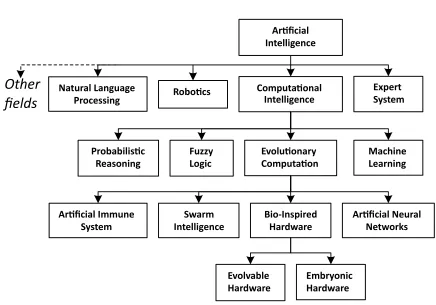
As shown in figure 1.1, computational intelligence is a subfield of artificial intelligence
that studies the mechanisms that enable intelligent behavior in complex and changing
environments [19]. The main focus of computational intelligence is to design and utilize
heuristic algorithms to solve complex real-world problems. The branches of this field
are machine learning, evolutionary computation, fuzzy logic, and probabilistic reasoning.
Evolutionary computation is the field in which the theory of evolution is used in
comput-ing systems. Its main areas are artificial neural networks, bio-inspired hardware, swarm
Ar cial
Intelligence
Computaonal
Intelligence
Expert System
Robocs
Evoluonary
Computaon
Ar cial Neural
Networks Machine Learning Fuzzy
Logic
Probabilisc
Reasoning
Ar cial Immune
System
Evolvable Hardware
Bio-Inspired Hardware
Embryonic Hardware Swarm
Intelligence Natural Language
Processing
Other
elds
Figure 1.1: Evolvable hardware and embryonic hardware are the main branches of bio-inspired hardware.
inspired hardware, is the research domain that relates the natural principles with electronic
systems. Evolvable hardware and embryonic hardware (EmHW) are the two main types of
bio-inspired hardware [20].
Evolvable hardware is defined as a hardware system that is capable of real-time
adapta-tion by reconfiguring internal hardware dynamically and autonomously [21]. Conversely,
EmHW can be defined as a hardware system with self-healing capability. Self-healing
(self-diagnosis, self-repair ability, or self-replication) is accomplished by in-cell failure
detection mechanisms, such as double modular redundancy or triple modular redundancy
[22], or out-of-cell mechanisms, where nearby cells can detect failing cells [20]. Since
discussed here.
1.1
Evolvable Hardware (EHW)
Evolvable hardware1is the field in which biological concepts are implemented in electrical
hardware using computer science algorithms, as shown in figure 1.2.
Figure 1.2: EHW is the field where biology, electrical engineering, and computer science meet.
The applications of EHW are classified into two main categories:
• EHW for Solving Design Problems: For complicated design problems, EHW can be
used to find a solution based on a set of specified criteria. The environment where the
EHW is running is generally fully described, and the output is deterministic. Since
the search space is large (2N, where N >100) and the EHW is often running in an
extrinsic mode (e.g., simulation), finding a solution typically takes a few days up
to weeks depending on the size of the search space, the complexity of the problem,
1Unfortunately, in many studies, evolvable hardware, evolutionary computation, artificial evolution, and
and the objective function. At the end of the evolution, many possible solutions
may be generated, but only one solution must be selected to be implemented on
hardware. Most of the early applications of EHW can be categorized in this category
[23, 24, 25, 26, 27].
• EHW for Online Adaptation: For applications with a changing environment, EHW
can be used to improve adaptivity at different levels, including fault detection and
tolerance. EHW is fast because it is often running in an intrinsic mode (online mode,
i.e., on hardware) and evolution is completely autonomous. Running in this mode
requires reconfigurable hardware platforms, which were not common until recently.
Therefore, many of these implementations are recent, as in [28, 1, 29, 30].
1.2
Main Components of Evolvable Hardware
As shown in figure 1.3, EHW consists of two components: a reconfigurable hardware core
and an evolutionary algorithm – the body and the brain.
Recongurable
Hardware Core
EHW Components
Evoluonary
Algorithm
1.2.1 Reconfigurable Hardware Core
A reconfigurable hardware core is the medium to embody possible solutions generated by
the evolutionary algorithm. The hardware core can be implemented in one of four possible
architectures:
1. Programmable logic devices used for digital designs.
2. Field-programmable analog arrays (FPAAs) used for analog designs.
3. Field-programmable transistor arrays (FPTAs) used for low-level mixed signal
de-signs.
4. Custom hardware architectures used for application-specific digital, analog, or mixed
systems.
Since the focus of our research is digital systems, programmable logic devices,
specif-ically field-programmable gate arrays (FPGAs), and digital custom hardware architectures
will be discussed in Chapter 2 in more detail.
A hardware architecture is considered to be a reconfigurable hardware core if it meets
certain requirements, including the following:
• Supporting reconfiguration multiple times – the architecture can be reconfigured
many or unlimited times.
• Supporting fast reconfiguration – since the search space is vast and millions of
re-configurations are needed, the reconfiguration speed is critical.
• Supporting partial reconfiguration – reconfiguration can occur partially on a
subre-gion of the programmable logic (called dynamic resubre-gion) without the need for
reconfiguration, where small regions of the programmable logic are reprogrammed
independently.
• Supporting dynamic reconfiguration – reconfiguring a (dynamic) region of a system
should not affect other (static) regions.
• Being inexpensive, flexible, and reliable – general requirements for any usable
archi-tecture.
1.2.2 Evolutionary Algorithms (EAs)
In biology literature,evolutionis defined as the change that occurs on inherited
characteris-tics of populations over consecutive generations to better adapt to the environment [31]. In
EHW, the term gene is used to represent a building block of a chromosome that represents
the aggregation of heredity information. Chromosomes are collections of genes, and the
collection of chromosomes of an individual is called a genome. Genomes in EHW can
be represented by integers, real numbers, strings, graphs, or trees and can fully describe
an individual (solution) [13]. Figure 1.4 shows the evolution cycle in biology with the
equivalent cycle in electronics. Evolution is achieved by heuristic algorithms, algorithms
that trade solution optimality for speed – evolutionary algorithms.
Evolutionary algorithmsare bio-inspired computer algorithms that feature natural
evo-lution and self-adaptation. These are search and optimization algorithms that attempt to
find optimal (or at least suboptimal) solutions in a large search space where classical
search methods are too slow. The search process, also known as the evolution process,
is performed iteratively usinggenetic operatorsand one or moreevaluation functions. EAs
Figure 1.4: Evolution cycle between (a) biology and (b) electronics [1].
that re-running the search process results in finding different solutions. The subfunctions
for an EA can be listed as follows:
• Representation: EA has to determine how to represent a hardware solution as a
genome. In other words, a decoding function or criterion needs to be defined that
allows mapping between two domains: the genotype (genome in the solution space)
and phenotype (individual in the problem space). For example, for a digital circuit
design, the genotype – a genome in the EA domain – can be represented by a string of
bits, while the phenotype – an individual in electronics – might be configuration data
for a circuit. Henceforth, genome, individual, and solution will used interchangeably
in this work.
• Population: the collection of individuals in a generation is called population. It is
generally fixed in size during evolution. The EA has to determine how to generate
generational, where a population is erased and recreated after every generation, and
overlapping, where a population is modified after every generation [32]. Population
diversity is a critical aspect of a successful EA.
• Evaluation function(also called fitness function or objective function): the EA has
to determine how to evaluate individuals. In other words, a fitness function needs
to be defined. A fitness function is a gauge of how close an individual is to meeting
the design specifications. In some applications, multiple fitness functions are defined.
Fitness functions are discussed in section 3.3. There are three methods to evaluate the
fitness in EHW: extrinsic [33], intrinsic [34], and mixtrinsic [35], which are discussed
in the following section.
• Genetic operators (also called variation operators): the EA has to determine how
genomes are raised and evolved in generations. These operators are selection,
muta-tion and crossover, and they are discussed in secmuta-tion 3.2.
• Termination condition: the EA has to determine when to stop evolution, e.g., after
evaluating a certain number of genomes or achieving a certain quality goal (i.e.,
fitness value).
Hardware Evolution Types
The type of evolution is determined by where individuals are evaluated, i.e., software and/or
hardware models, and where the EA and fitness function are running. The three types are
described as follows:
Extrinsic evolutionis performed when an individual is modeled and evaluated on
soft-ware. Subsequently, the solution with the best fitness is implemented in hardsoft-ware. The
equally. In digital circuits, the software modeling can represent hardware with almost
complete correctness [36, 37, 38, 39]. An example of this method is using a hardware
description language (HDL) to simulate a circuit; then, based on the simulation results, the
fittest circuit is replicated in hardware.
Intrinsic evolution is performed directly on hardware where a genome is modeled
and evaluated on hardware. This method requires hardware with a fast reconfiguration
time. Intrinsic evolution is fast, and since there is no software modeling, there is no
hardware-to-software functional mismatching. There are four subcategories of intrinsic
EHW, which are based on where the EA and fitness evaluation are performed. These
are intrinsic, complete intrinsic, multi-chip intrinsic, and multi-board intrinsic, which are
summarized in figure 1.5.
Mixtrinsic evolutionis where individual solutions are modeled in a mixture of hardware
and software models. This method solves the extrinsic evolution issue of mismatching by
guaranteeing that a solution behaves well on hardware and during simulation.
Comple-mentary mixtrinsic and combined mixtrinsic are the two modes of operation for mixtrinsic
evolution [35]. Complementary mixtrinsic evolution is where a genome is assigned
ran-domly to a hardware model or software model. Combined mixtrinsic evolution is where
a genome is modeled in software and hardware and an average fitness value is calculated
when the two fitness values are mismatching.
1.3
Applications of EHW
The applications of EHW can be seen in many fields. This is because EHW allows
on-line adaptation to environment changes, solves complex problems, and increases system
Figure 1.5: Intrinsic EHW types based on where the EA is running [2].
[40, 41, 42, 43, 44] and digital circuit design [45, 46, 47, 48, 49, 50, 51]. EHW is also used
in image processing applications, such as developing adaptive filters [30, 52] and pattern
recognition [53, 54, 21, 55]. In other cases, EHW is used to evolve systems with fault
tol-erance capabilities, such as fault-tolerant circuits [56, 57, 58], circuits with fault toltol-erance
using natural redundancy [59], fault-tolerant image processors [60], and high-reliability
space applications [61]. EHW has been used in solving some hard problems, such as
the classical applications in [23] and NP-complete problems [62]. In the communication
systems domain, EHW is used to adapt to different communication protocols [63] and
autonomously optimize signal strength [64]. In computer hardware, EHWs have been used
[67, 68, 15, 69, 70, 71], robotic and control systems [72, 73, 74, 75], data mining [76, 77],
data compression [78, 79], data cryptography [80, 81, 82], medical applications [83], many
analog applications as summarized on page 68 of [13], and many others.
1.4
Motivation and Research Objectives
The objectives and main areas proposed for investigation are summarized as follows:
1. Developing an autonomous system with accelerated evolution: The term accelerated
evolution represents many subgoals, including developing a fast hardware core and
an efficient evolutionary algorithm. In our work, we develop a set of EHWs where
the hardware core and evolutionary algorithm are cooperating to improve evolution.
2. Achieving fast reconfiguration without sacrificing resources: Although this objective
can be a subgoal of the previous one, fast reconfiguration is set as a goal by itself
because reconfiguration with less overhead is a vital goal of EHW. Because there are
advantages and disadvantages for both common types of reconfiguration schemes,
a hybrid scheme is created that combines the merits of both schemes while still
avoiding their drawbacks.
3. Improving reliability by fault detection and tolerance: In general, on an EHW system,
self-adaptation is the main target, which is in contrast to EmHW, where self-healing
is the main goal. The flexibility of the designed system allows for a simple yet
efficient fault detection and tolerance mechanism.
4. Improving genetic algorithm to perform better genetic operations: The genetic
core. Although we believe it is a desirable abstraction, some modifications can still
be made to make them perform better on systolic arrays.
1.5
Contributions
An efficient and complete intrinsic EHW platform is proposed. The system can be enclosed
entirely on a commercial low-cost system-on-chip (SoC). The presented system features
a novel FPGA-based reconfigurable hardware core (called HexArray). HexArray offers a
high level of routing flexibility and combines the merits of the two common reconfiguration
schemes.
In addition, the proposed system also features a novel genome-aware genetic algorithm
(called GAGA), which is a context-aware genetic algorithm designed specifically for
sys-tolic arrays (such as HexArray). Moreover, some of the introduced genetic operations
are applicable to a wide range of evolutionary algorithms and evolvable architectures.
A collection of experiments shows that the proposed GAGA operators truly accelerate
evolution. Additionally, the new architecture supports a simple but robust fault detection
and tolerance mechanism. Moreover, a technique is proposed that allows the system to
evaluate genomes while the arrays are being reconfigured.
In this work, we propose a novel EHW platform based on a new reconfigurable
hard-ware core and evolutionary algorithm. Furthermore, additional features have been proposed
that exploit the features of the new platform. The contributions in this dissertation are
summarized as follows:
1. A novel processing element (called HexCell).
(a) A novel hybrid reconfiguration scheme.
(b) A novel fault detection and tolerance mechanism.
(c) A novel evolve-while-reconfigure technique.
3. A novel evolutionary algorithm (called GAGA) featuring the following:
(a) A novel genome-aware constrained selection (GAC selection).
(b) A novel genome-aware mutation (GAM).
(c) A novel genome-aware crossover (GAX) running in three different modes.
(d) A novel genome-aware pruner (GAP).
1.6
Dissertation Overview
Since an EHW is proposed in this dissertation, the first EHW component is discussed
in Chapter 2. The discussion starts with the properties of reconfigurable hardware cores
followed by the common architectures in the field. The next chapter, Chapter 3, discusses
the other component of an EHW, evolutionary algorithms. This chapter explores the means
of EAs, which are genetic operators and the fitness functions. Different common types of
EAs are then briefly considered, with a special emphasis on genetic algorithms. Different
classifications of EHWs are presented in Chapter 4, along with a variety of FPGA-based
and custom-hardware implementations with a special focus on the systolic arrays.
The contributions of this work are presented in Chapter 5. The discussion starts with
an early implementation of the proposed system in software – HexArray Simulator. The
simulator served as a proof of concept, but discussing it permits a high-level understanding
of the system without involving much complexity. In the next section, section 5.3, the
part (section 5.4) will be dedicated to presenting the GAGA and its utility functions and
genome-aware genetic operators. Additional features enabled by the new system are
pro-vided in section 5.6. A comparison between HexArray and the state-of-the-art systolic
array is presented at the end of the chapter.
Chapter 6 consists of a comprehensive set of experiments to test the new platform;
the discussion in this part of the chapter is limited to the evolution speed (i.e., for a
fixed number of genomes, what is the best fitness achieved). Section 6.3 discusses the
implementation details, timing analysis, and resource utilization.
Finally, we conclude this dissertation by summarizing the contributions of this work.
“What is the value of HexCell, HexArray, GAC Selection, GAM, and GAX?” will also be
CHAPTER 2
RECONFIGURABLE HARDWARE CORE
2.1
Introduction
To develop an EHW system, a reconfigurable architecture and an evolutionary algorithm
are needed. A reconfigurable architecture is a hardware system that can be programmed by
the user or application. The hardware system is used to realize solutions suggested by the
EA.
There are several technologies that enable programmability (and re-programmability).
Early programmable architectures used programmable read-only memory (PROM). Since
PROM was a one-time programmable memory, erasable PROM (EPROM) was introduced
to allow for reprogramming several times. However, EPROM was erasable by long
ex-posure to ultraviolet light, e.g., several minutes using an ultraviolet eraser machine.
Con-sequently, electrically EPROM (EEPROM) was invented, which accelerated the erasing
process and eliminated the need for an external device to erase the memory. Subsequently,
flash memories were used. A flash device is a matrix of EEPROMs that are segmented
into smaller blocks that can be independently erased. One aspect of all previous
non-volatile devices is the limitation on how many times they can be reprogrammed. Another
reconfigurable device is static RAMs (SRAMs), which are volatile devices used for fast
configuration and unlimited reconfigurations. As mentioned previously in section 1.2.1,
reconfigured multiple times.
2.2
Properties of Reconfigurable Hardware Cores
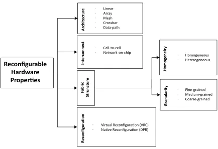
As shown in figure 2.1, there are several ways to characterize reconfigurable
architec-tures, including architecture, interconnect, fabric structure and reconfiguration schemes.
Although these terms are tightly connected, some key differences can still be outlined, as
follows:
Architecture
Recon gurable
Hardware
Proper es
Fabric
Strunctu
re
Inte
rconnect
Homogeneit
y
Granularit
y
Reconfigurati
on
∙ Linear
∙ Array
∙ Mesh
∙ Crossbar
∙ Data-path
∙ Cell-to-cell
∙ Network-on-chip
∙ Homogeneous
∙ Heterogeneous
∙ Fine-grained
∙ Medium-grained
∙ Coarse-grained
∙ Virtual Reconguraon (VRC)
∙ Nave Reconguraon (DPR)
2.2.1 Architecture
Reconfigurable architectures generally have building blocks that are connected in a certain
way – called the architecture of the platform. In other words, the architecture describes
the connectivity scheme of processing elements (PEs) in a reconfigurable architecture.
Common architectures are as follows:
1. Linear: PEs are connected linearly (without any dynamic routing). The connection,
however, does not need to be to the nearest neighboring PEs.
2. Array: PEs are placed and connected in a regular manner.
3. Mesh: Array architectures can be further classified as a mesh architecture when the
neighboring PEs are grouped in “super-blocks” to reduce the routing density. In
this architecture, high-density routing is maintained intra-super-blocks while reduced
inter-super-blocks.
4. Crossbar: Architectures that were classified as mesh can be classified as crossbar
when extra (dynamic) routing resources are available between the super-blocks.
5. Datapath: An architecture is said to be a datapath when the routing of data is
con-trolled at the bus-level rather than at the bit-level. This is typically for course-grained
architectures such as x-bit processors, where the routing is controlled at the x-bit
level.
2.2.2 Interconnect
The interconnect of an architecture describes the mechanism of the data flow. Depending on
(for fine-grained logic) or as complex as a network-on-chip (for coarse-grained logic),
where data are sent as network packets.
2.2.3 Fabric Structure
In terms ofhomogeneity, an architecture is classified as homogeneous when all the
config-urable blocks are identical in function and arranged in a regular manner, or it is classified
as heterogeneous when specialized blocks exist. Conversely, the fabric structure can also
be defined in terms of granularity: fine-grained (e.g., array of transistors or logic gates),
medium-grained (e.g., array of basic processing units such as adder, subtractor, or
multi-plexer) or coarse-grained (e.g., array of DSP cores or processors).
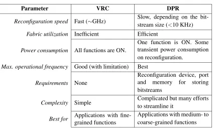
2.2.4 Reconfiguration Schemes
In terms of reconfigurability, the hardware core can be reconfigured in one of two methods:
virtual reconfiguration circuit (VRC) or native reconfiguration (often called dynamic partial
reconfiguration, DPR), as shown in figure 2.2; additionally, a comparison is presented in
table 2.1.
(a)VRC (b)DPR
Virtual Reconfiguration Circuit (VRC)
Virtual reconfiguration circuit is a method where the evolutionary algorithm switches
be-tween a set of existing functions that are physically implemented in hardware. This method
is fast since the delay only depends on the time consumed by switching between functions,
but it is not space or power efficient. Moreover, in some applications, VRC may result in
lowering the maximum operational frequency [84]. Most of the early EHW systems were
VRC-based for three reasons: (1) VRC is a simple method to be implemented. (2) VRC
works well for fine-grained functions. (3) Until recently, the technology did not support
any other way of reconfiguration.
Dynamic Partial Reconfiguration (DPR)
Dynamic partial reconfiguration is the method of reconfiguring or reprogramming a
dy-namic region of an FPGA fabric using a bitstream from a library of pre-compiled
func-tions. Because the dynamic region is relatively large, DPR is fairly slow for the required
speed of most real-world applications. However, DPR is power and space efficient, and it
may be the only practical choice for applications with coarse-grained functions. Initially,
DPR was feasible using low-level bitstream manipulation methods [85, 56] enabled by
open architectures, bitstream reverse engineering and/or some open-source application
programming interfaces (APIs) such as TORC [86] and RapidSmith [87]. A low-level
bitstream manipulation method can be unsafe and complicated, particularly on recent
FP-GAs [45]. Currently, major FPGA vendors support native run-time reconfiguration, but
with some limitations, such as complex design flow and unsupported bitstream relocation.
Despite these limitations, many successful EHW implementations have been proposed
Table 2.1: Comparison of VRC and DPR.
Parameter VRC DPR
Reconfiguration speed Fast (∼GHz) Slow, depending on the
bit-stream size (<10 KHz)
Fabric utilization Inefficient Efficient
Power consumption All functions are ON.
One function is ON. Some transient power consumption on reconfiguration.
Max. operational frequency Good (with limitation) Best
Requirements None
Reconfiguration device, port
and memory for storing
bitstreams
Complexity Simple Complicated but many efforts
to streamline it
Best for Applications with
fine-grained functions
Applications with medium- to coarse-grained functions
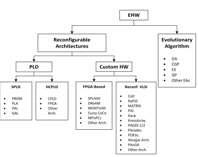
2.3
Reconfigurable Architectures
Reconfigurable architectures can be classified into two categories: commercial and custom
architectures, as shown in figure 2.3. Commercial programmable architectures are
dis-cussed first. Then, custom reconfigurable architectures are disdis-cussed, where some EHWs
utilize FPGAs to realize the final system architecture.
2.3.1 Commercial Simple Programmable Logic Devices
After the birth of PROMs and because of the high demand for compact and flexible “glue
logic” architectures, a new family of devices were created. Programmable logic devices
(PLDs) come in many forms, as shown in figure 2.3, but they all serve one purpose. PLDs
SPLD
PLD
Reconfigurable Architectures
Custom HW
HCPLD FPGA-Based Reconf. VLSI
EHW
Evolutionary Algorithm
· PROM
· PLA
· PAL
· GAL
· CPLD
· FPGA
· Other
Arch.
· SPLASH
· DReAM
· MONTIUM
· Fuzzy CoCo
· MPoPCs
· Other Arch.
· Colt
· RaPiD
· MATRIX
· PIG
· Garp
· KressArray
· PADDI-1/2
· Pleiades
· POEtic
· Alnajjar Arch.
· PAnDA
· Other Arch.
· GA
· CGP
· ES
· GP
· Other EAs
Figure 2.3: Classifications of reconfigurable architectures.
Simple Programmable Logic Devices
Simple programmable logic devices (SPLDs) are the simplest reconfigurable arrays with a
relatively low amount of simple logic (<1000 gates). These devices contain a set of fully
connected macrocells, where each macrocell contains a mix of simple gates and flip-flops,
which are sufficient to realize basic functions in the product-of-sums (or sum-of-products)
canonical form. The SPLD consists of three main blocks: the input block, AND plane, and
...
...
...
InputsIBuffers & Inverters
AND Plane
OR
Plane Outputs
...
Figure 2.4: Simplified SPLD, adapted from [4].
Programmable Read-Only Memory (PROM)
The simplest form of programmable devices is PROM, which is a block of programmable
memory that stores truth table data of the intended logical design. The input to the PROM
works as an address to the memory, and the stored data serves as the output. An example
of a PROM is shown in figure 2.5. For PROMs, the user can only program the content
of the memory and is unable to change the input or output routing. Due to the discussed
limitations, flexibility and scalability are the major drawbacks of PROMs.
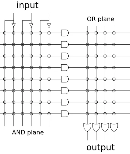
Programmable Logic Arrays (PLAs)
Programmable logic arrays are another type of SPLD. PLAs were introduced in the early
1970s by Texas Instruments based on read-only associative memory (ROAM) to solve the
drawbacks from which PROMs suffered. The main feature of PLAs is that both of their
planes (i.e., AND plane and OR plane) are programmable, as shown in figure 2.6. The
architecture of the input interconnect allows for more flexibility on the input ports. Since
the two programmable links were slow OR gates, PLAs were slower than PROMs and did
not gain popularity.
input
output
AND plane
OR plane
Figure 2.6: PLA has a programmable AND plane and a programmable OR plane.
Programmable Array Logic (PAL)
Programmable array logic was introduced in 1978 by Monolithic Memories Inc. [92]. In
the input connection matrix, as shown in figure 2.7. Since there is a single (AND gate)
link in the PALs compared with two (OR gate) links in the PLAs, PALs were faster than
PLAs. However, PALs were less reprogrammable than PLAs since they had AND-based
programmable links. Although a hardwired output indicates a flexibility limitation on what
logical equations the circuit can represent in comparison with the former PLA devices, the
additional programmable loopback interconnect in PALs improved their flexibility because
it allowed realization of multi-level canonical forms.
Figure 2.7: PAL architecture with loopback wiring to improve flexibility [6].
Generic Array Logic (GAL)
Generic array logic, introduced by Lattice Semiconductor in 1985, was the next generation
of PALs. The main features showcased were the integration of CMOS technology and
improved reconfigurability, where the device can be reconfigured many times using a
2.3.2 Commercial High-Capacity Programmable Logic Devices
Another branch of PLDs consists of high-capacity programmable logic devices (HCPLDs).
HCPLDs include complex programmable logic devices (CPLDs), FPGAs, and other
com-mercial programmable architectures.
Complex Programmable Logic Devices (CPLDs)
A CPLD is a high-density programmable logic device that is more complex (larger) than
PALs but less complex than FPGAs. In contrast to FPGAs, CPLDs have a non-volatile
EEPROM-based configuration memory that makes them fast to boot but slow to be
re-programmed. Due to their simpler architecture, CPLDs have low pin-to-pin delays. A
simplified high-level block diagram for a CPLD is presented in figure 2.8. Macrocells are
the building blocks of CPLDs, which are relatively larger than the building blocks of
FP-GAs. However, a CPLD typically has less than a few hundred macrocells versus more than
ten thousand building blocks for FPGAs. Figure 2.9 shows MAX V, a CPLD manufactured
kc
ol
B
O/
I
Logic Block
Logic Block
Logic Block
Logic Block Interconnection Array
kc
ol
B
O/
I
by Altera. This device (5M40Z specifically) has 24 logic array blocks (LABs) stacked in
a 6x4 array with a MultiTrack interconnect in-between. Each LAB consists of 10 logic
elements (LEs). The structure of an LE is shown in figure 2.10. The typical equivalent
macrocells for 5M40Z is 32 macrocells, indicating that an LAB in this device is larger than
a typical macrocell.
Logic Array BLock (LAB)
MultiTrack Interconnect
MultiTrack Interconnect
Logic Element
Logic Element IOE
IOE
IOE IOE
Logic Element
Logic Element IOE
IOE
Logic Element
Logic Element
IOE IOE
Logic Element
Logic Element
Logic Element
Logic Element
IOE IOE
Logic Element
Logic Element
Figure 2.9: MAX V: a CPLD manufactured by Altera [7].
Field-Programmable Gate Arrays (FPGAs)
FPGAs are integrated circuits designed to be configured by customers in the field. An
dig-DirectLink interconnect from adjacent LAB or IOE
DirectLink interconnect to adjacent LAB or IOE
RowInterconnect
ColumnInterconnect
Local Interconnect LAB
DirectLink interconnect from adjacent LAB or IOE
DirectLink interconnect to adjacent LAB or IOE
Fast I/O connection to IOE(1)
Fast I/O connection to IOE(1)
LE0
LE1
LE2
LE3
LE4
LE6
LE7
LE8
LE9 LE5
LogicElement
Figure 2.10: LABs are the building blocks of CPLDs. Each LAB has 10 LEs [7].
ital signal processor blocks (DSPs), and other hard-cores (occasionally hard-IP cores). The
programmable blocks are arranged in columns with complex intermediate interconnects.
The programmable array is surrounded by programmable input/output blocks (IOBs). A
simplified FPGA layout is shown in figure 2.11.
CLBs are the main building blocks of FPGAs. In the case of the Xilinx 7 series, a CLB,
as shown in figure 2.12, consists of two slices, where each slice has four 6-input look-up
tables (LUTs), eight flip-flops, multiplexers, and arithmetic carry logic. The arrangement
of programmable blocks for this FPGA is called the ASMBL (advanced silicon modular
block) architecture, as shown in figure 2.13.
Most of the FPGAs’ configuration memory is SRAM-based. The configuration of an
I/O Block
Interconnecting Switches
Logic Block
Figure 2.11: Simplified FPGA block diagram [4].
using an HDL, such as VHSIC (very high speed integrated circuit) hardware description
language (VHDL) or Verilog using electronic design automation (EDA) tools provided by
the FPGA vendor. This process includes many subprocesses, such as elaboration, synthesis,
placement, routing, implementation, bitstream generation, and optionally simulation.
There are two types of bitstreams: full-chip bitstream and partial bitstream. The
full-chip bitstream is for configuring the entire chip, where the device functionality is
inter-rupted while it is being programmed. Conversely, partial bitstream is where only a subarray
of the logic (called dynamic partition) is reprogrammed without interrupting the operation
of the remaining part of the array. The size of the partial bitstream depends on the size of the
dynamic partition, which determines the speed of reconfiguration. Xilinx 7 series devices
(specifically Zynq-7000) support several ways to configure the programmable logic, such
as using the processor configuration access port (PCAP), joint test action group (JTAG),
Switch Matrix
Slice(1) COUT COUT
CIN CIN
Slice(0) CLB
Figure 2.12: Two slices per CLB, Xilinx 7 series [8].
module (DevC), which has an embedded direct memory access (DMA) controller capable
of initiating data transfers from the external memory to the fabric configuration memory.
Therefore, PCAP does not need any hardware instantiations on the programmable logic.
The maximum configuration speed achieved by PCAP is 128 MB/sec. ICAP, in contrast,
requires instantiating a Hardware ICAP (HWICAP) module in the programmable logic.
Although the theoretical maximum speed of ICAP is 400 MB/s, the maximum achievable
speed is 67 MB/sec using conventional DMA-dependent transactions. Vipin et al. proposed
an efficient management system, ZyCAP, that increases ICAP performance to 382 MB/sec
[93].
Other Commercial Reconfigurable Platforms
There are many commercial reconfigurable architectures. One example is D-Fabrix
manu-factured by Panasonic, which is a low-power ASIC aimed at embedded multimedia
Column Based ASMBL Architecture
Feature Options
Domain A Domain B Domain C
Applications Applications Applications
Logic(SLICEL)
Logic(SLICEM)
DSP
Memory
Clock Management Tile
Global Clock
High-performance I/O
High-range I/O
Integrated IP
Mixed Signal
Transceivers
Figure 2.13: Variety of programmable logic blocks are arranged in a column-style, ASMBL architecture [8].
on the CHESS reconfigurable platform developed by Hewlett Packard Labs [95]. The
device specifications are not disclosed. Another example of commercial reconfigurable
architectures is the PACT XPP-III architecture used in low-power irregular
control-flow-dominated streaming algorithms [13]. The XPP-III architecture is based on a hierarchical
array of sequential coarse-grained processors optimized to run in different types of
par-allelism [96]. QuickSilver Adapt2400 [97], Coherent Logix HyperX [98], and Adapteva
Parallella [99] are examples of other common commercial reconfigurable architectures.
2.3.3 Custom Architectures
Custom architectures include two branches. The first branch is for FPGA-based
archi-tectures, but here it does not mean using the FPGA fabric (e.g., LUTs or CLBs) as the
![Figure 1.4: Evolution cycle between (a) biology and (b) electronics [1].](https://thumb-us.123doks.com/thumbv2/123dok_us/8919918.1841002/40.612.109.541.100.310/figure-evolution-cycle-biology-b-electronics.webp)
![Figure 1.5: Intrinsic EHW types based on where the EA is running [2].](https://thumb-us.123doks.com/thumbv2/123dok_us/8919918.1841002/43.612.178.466.100.391/figure-intrinsic-ehw-types-based-ea-running.webp)
![Figure 2.9: MAX V: a CPLD manufactured by Altera [7].](https://thumb-us.123doks.com/thumbv2/123dok_us/8919918.1841002/59.612.146.505.226.552/figure-max-v-cpld-manufactured-altera.webp)
![Figure 2.10: LABs are the building blocks of CPLDs. Each LAB has 10 LEs [7].](https://thumb-us.123doks.com/thumbv2/123dok_us/8919918.1841002/60.612.110.539.100.372/figure-labs-building-blocks-cplds-lab-les.webp)
![Figure 2.11: Simplified FPGA block diagram [4].](https://thumb-us.123doks.com/thumbv2/123dok_us/8919918.1841002/61.612.181.465.106.320/figure-simplied-fpga-block-diagram.webp)
