Cryptanalysis of Full RIPEMD-128

Cryptanalysis of Full RIPEMD-128

Franck Landelle

1

_{and Thomas Peyrin}

2

,?

1

_{DGA MI, France}

2

Division of Mathematical Sciences, School of Physical and Mathematical Sciences,

Nanyang Technological University, Singapore

[email protected]

[email protected]

Abstract.

In this article we propose a new cryptanalysis method for double-branch hash functions that we

apply on the standard

RIPEMD-128

, greatly improving over know results. Namely, we were able to build a very

good differential path by placing one non-linear differential part in each computation branch of the

RIPEMD-128

compression function, but not necessarily in the early steps. In order to handle the low differential probability

induced by the non-linear part located in later steps, we propose a new method for using the freedom degrees,

by attacking each branch separately and then merging them with free message blocks. Overall, we present

the first collision attack on the full

RIPEMD-128

compression function as well as the first distinguisher on the

full

RIPEMD-128

hash function. Experiments on reduced number of rounds were conducted, confirming our

reasoning and complexity analysis. Our results show that 16 years old

RIPEMD-128

, one of the last unbroken

primitives belonging to the

MD

-

SHA

family, might not be as secure as originally thought.

Key words:

RIPEMD-128, collision, distinguisher, compression function, hash function.

1

Introduction

Hash functions are among the most important basic primitives in cryptography, used in many applications such as

digital signatures, message integrity check and message authentication codes (MAC). Informally, a hash function

H

is a function that takes an arbitrarily long message

M

as input and outputs a fixed-length hash value of size

n

bits. Classical security requirements are collision resistance and (second)-preimage resistance. Namely, it should

be impossible for an adversary to find a collision (two distinct messages that lead to the same hash value) in less

than 2

n/

2

_{hash computations, or a (second)-preimage (a message hashing to a given challenge) in less than 2}

n

hash computations. More complex security properties can be considered up to the point where the hash function

should be indistinguishable from a random oracle, thus presenting no weakness whatsoever. Most standardized

hash functions are based upon the Merkle-Damg˚

ard paradigm [18, 6] and iterate a compression function

h

with

fixed input size to handle arbitrarily long messages. The compression function itself should ensure equivalent

security properties in order for the hash function to inherit from them.

Recent impressive progresses in cryptanalysis [29, 27, 28, 26] led to the fall of most standardized hash primitives,

such as

MD4,

MD5,

SHA-0

and

SHA-1. All these algorithms share the same design rationale for their compression

functions (i.e. they incorporate additions, rotations, xors and boolean functions in an unbalanced Feistel network),

and we usually refer to them as the

MD-SHA

family. As of today, among this family only

SHA-2,

RIPEMD-128

and

RIPEMD-160

remain unbroken, but the rapid improvement of the attacks decided the NIST to organize a 4-year

SHA-3

competition in order to design a new hash function, eventually leading to the selection of

Keccak

[1]. This

choice was justified partly by the fact that

Keccak

is built upon a completely different design rationale than the

MD-SHA

family. Yet, we can not expect the industry to move quickly to

SHA-3

unless a real issue is identified in

current hash primitives. Therefore, the

SHA-3

competition monopolizing most of the cryptanalysis power during

the last four years, it is now crucial to continue the study of the unbroken

MD-SHA

members.

The notation

RIPEMD

represents several distinct hash functions related to the

MD-SHA-family, the first

represen-tative being

RIPEMD-0

[2] that was recommended in 1992 by the European

RACE Integrity Primitives Evaluation

(RIPE) consortium. Its compression function basically consists in two

MD4-like [20] functions computed in parallel

(but with different constant additions for the two branches), with 48 steps in total. Early cryptanalysis by

Dob-bertin on a reduced version of the compression function [9] seemed to indicate that

RIPEMD-0

was a weak function

and this was fully confirmed much later by Wang

et al.

[26] who showed that one can find a collision for the full

RIPEMD-0

hash function with as few as 2

16

_{computations.}

However, in 1996, due to the cryptanalysis advances on

MD4

and on the compression function of

RIPEMD-0,

the original

RIPEMD-0

was reinforced by Dobbertin, Bosselaers and Preneel [10] to create two stronger primitives

RIPEMD-128

and

RIPEMD-160, with 128

/

160-bit output and 64

/

80 steps respectively (two other less known 256

and 320-bit output variants

RIPEMD-256

and

RIPEMD-320

were also proposed, but with a claimed security level

equivalent to an ideal hash function with a twice smaller output size). The main novelty compared to

RIPEMD-0

is that the two computation branches were made much more distinct by using not only different constants, but

?

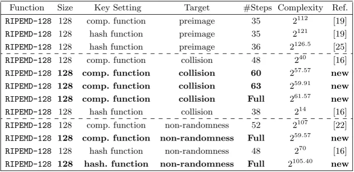
Table 1.

Summary of known and new results on

RIPEMD-128

hash function

Function

Size

Key Setting

Target

#Steps Complexity

Ref.

RIPEMD-128

128

comp. function

preimage

35

2

112

_[19]

RIPEMD-128

128

hash function

preimage

35

2

121

[19]

RIPEMD-128

128

hash function

preimage

36

2

126.5

[25]

RIPEMD-128

128

comp. function

collision

48

2

40

[16]

RIPEMD-128

128

comp. function

collision

60

2

57.57

new

RIPEMD-128

128

comp. function

collision

63

2

59.91

new

RIPEMD-128

128

comp. function

collision

Full

2

61.57

_new

RIPEMD-128

128

hash function

collision

38

2

14

[16]

RIPEMD-128

128

comp. function

non-randomness

52

2

107

_[22]

RIPEMD-128

128

comp. function

non-randomness

Full

2

59.57

new

RIPEMD-128

128

hash function

non-randomness

48

2

70

[16]

RIPEMD-128

128

hash. function

non-randomness

Full

2

105.40

new

also different rotation values and boolean functions, which greatly hardens the attacker’s task in finding good

differential paths for both branches at a time. The security seems to have indeed increased since as of today no

attack is known on the full

RIPEMD-128

or

RIPEMD-160

compression/hash functions and the two primitives are

worldwide ISO/IEC standards [12].

Even though no result is known on the full

RIPEMD-128

and

RIPEMD-160

compression/hash functions yet,

many analysis were conducted in the recent years. In [17], a preliminary study checked up to what extent can

the known attacks [26] on

RIPEMD-0

apply to

RIPEMD-128

and

RIPEMD-160. Then, following the extensive work

on preimage attacks for

MD-SHA

family, [21, 19, 25] describe high complexity preimage attacks on up to 36 steps

of

RIPEMD-128

and 31 steps of

RIPEMD-160. Collision attacks were considered in [16] for

RIPEMD-128

and in [15]

for

RIPEMD-160, with 48 and 36 steps broken respectively. Finally, distinguishers based on non-random properties

such as second-order collisions are given in [16, 22, 15], reaching about 50 steps with a very high complexity.

Our contributions.

In this article, we introduce a new type of differential path for

RIPEMD-128

using one

non-linear differential trail for both left and right branches and, in contrary to previous work, not necessarily located

in the early steps (Section 3). The important differential complexity cost of these two parts is mostly avoided by

using the freedom degrees in a novel way: some message words are used to handle the non-linear parts in both

branches and the remaining ones are used to merge the internal states of the two branches (Section 4). Overall, we

obtain the first cryptanalysis of the full 64-round

RIPEMD-128

hash and compression functions. Namely, we provide

a distinguisher based on a differential property for both the full 64-round

RIPEMD-128

compression function and

hash function (Section 5). Previously best-known results for non-randomness properties only applied to 52 steps

of the compression function, 48 steps of the hash function. More importantly, we also derive a semi-free-start

collision attack on the full

RIPEMD-128

compression function (Section 5), significantly improving the previous

free-start collision attack on 48 steps. Any further improvement of our techniques is likely to provide a practical

semi-free-start collision attack on the

RIPEMD-128

compression function. In order to increase the confidence in our

reasoning, we implemented independently the two main parts of the attack (the merge and the probabilistic part)

and the observed complexity matched our predictions. Our results and previous works complexities are given in

Table 1 for comparison.

2

Description of

RIPEMD-128

RIPEMD-128

[10] is a 128-bit hash function that uses the Merkle-Damg˚

ard construction as domain extension

algorithm: the hash function is built by iterating a 128-bit compression function

h

that takes as input a 512-bit

message block

m

i

and a 128-bit chaining variable

cv

i:

cv

i

+1

=

h

(

cv

i

, m

i)

where the message

m

to hash is padded beforehand to a multiple of 512 bits

3

_{and the first chaining variable is set}

to a predetermined initial value

cv

0

=

IV

(given in Table 2 of Appendix A).

We refer to [10] for a complete description of

RIPEMD-128. In the rest of this article, we denote by [

Z

]i

the

i

-th

bit of a word

Z

, starting the counting from 0.

and

represent the modular addition and subtraction on 32 bits,

and

⊕

,

∨

,

∧

, the bitwise “exclusive or”, the bitwise “or”, and the bitwise “and” function respectively.

3

The padding is the same as for

MD4

: a “

1

” is first appended to the message, then

x

“

0

” bits (with

x

= 512

−

(

|

m

|

+ 1 + 64

2.1

RIPEMD-128

compression function

The

RIPEMD-128

compression function is based on

MD4, with the particularity that it uses two parallel instances

of it. We differentiate these two computation branches by left and right branch and we denote by

X

i

(resp.

Y

i

)

the 32-bit word of left branch (resp. right branch) that will be updated during step

i

of the compression function.

The process is composed of 64 steps divided into 4 rounds of 16 steps each in both branches.

Initialization.

The 128-bit input chaining variable

cv

i

is divided into 4 words

h

i

of 32 bits each, that will be

used to initialize the left and right branch 128-bit internal state:

X

−3

=

h

0

X

−2

=

h

1

X

−1

=

h

2

X

0

=

h

3

Y

−3

=

h

0

Y

−2

=

h

1

Y

−1

=

h

2

Y

0

=

h

3

.

The message expansion.

The 512-bit input message block is divided into 16 words

M

i

of 32 bits each. Each

word

M

i

will be used once in every round in a permuted order (similarly to

MD4) and for both branches. We

denote by

W

_i

l

(resp.

W

_i

r

) the 32-bit expanded message word that will be used to update the left branch (resp.

right branch) during step

i

. We have for 0

≤

j

≤

3 and 0

≤

k

≤

15:

W

_j

l

_·16+

_k

=

M

_π

l

j

(

k

)

and

W

r

j

·16+

k

=

M

π

r j

(

k

)

where permutations

π

l

_j

and

π

r

_j

are given in Table 3 of Appendix A.

The step function.

At every step

i

, the registers

X

i

+1

and

Y

i

+1

are updated with functions

f

j

l

and

f

j

r

that

depends on the round

j

in which

i

belongs:

X

i

+1

= (

X

i

−3

Φ

l

j

(

X

i

, X

i

−1

, X

i

−2

)

W

i

l

K

l

j

)

<<<

s

l i

_,

Y

i

+1

= (

Y

i

−3

Φ

r

j

(

Y

i

, Y

i

−1

, Y

i

−2

)

W

i

r

K

r

j

)

<<<

s

r_i

_,

where

K

l

j

, K

j

r

are 32-bit constants defined for every round

j

and every branch,

s

l

i

, s

r

i

are rotation constants defined

for every step

i

and every branch,

Φ

l

j

, Φ

r

j

are 32-bit boolean functions defined for every round

j

and every branch.

All these constants and functions are given in Appendix A.

The finalization.

A finalization and a feed-forward is applied when all 64 steps have been computed in both

branches. The four 32-bit words

h

0

_i

composing the output chaining variable are finally obtained by:

h

0

₀

=

X

63

Y

62

h

1

h

0

1

=

X

62

Y

61

h

2

h

0

₂

=

X

61

Y

64

h

3

h

0

3

=

X

64

Y

63

h

0

.

3

A new family of differential paths for

RIPEMD-128

3.1

The general strategy

The first task for an attacker looking for collisions in some compression function is to set a good differential path.

In the case of

RIPEMD

and more generally double or multi-branches compression functions, this can be quite a

difficult task because the attacker has to find a good path for all branches at the same time. This is exactly what

multi-branches functions designers are hoping: it is unlikely that good differential paths exist in both branches

at the same time when the branches are made distinct enough (note that the weakness of

RIPEMD-0

is that both

branches are almost identical and the same differential path can be used for the two branches at the same time).

Differential paths in recent collision attacks on

MD-SHA

family are composed of two parts: a low probability

non-linear part in the first steps and a high probability linear part in the remaining ones. Only the latter will be

handled probabilistically and impact the overall complexity of the collision finding algorithm, since during the first

steps the attacker can choose message words independently. This strategy proved to be very effective because it

allows to find much better linear parts than before by relaxing many constraints on them. The previous approaches

for attacking

RIPEMD-128

[17, 16] are based on the same strategy, building good linear paths for both branches,

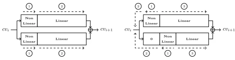
but without including the first round (i.e. the first 16 steps). The first round in each branch will be covered by

a non-linear differential path and this is depicted left in Figure 1. The collision search is then composed of two

subparts, the first handling the low-probability non-linear paths with the message blocks (step

1

and then the

cv

i

cv

i+1

Linear Non

Linear

1 2

Linear Non

Linear

1 2

cv

i

cv

i+1

0 Non Linear

Linear

1 3

2

Linear Non

Linear

1 3

2

Fig. 1.

The previous (left-hand side) and new (right-hand side) approach for collision search on double-branch compression

functions.

This differential path search strategy is natural when one will handle the non-linear parts in a classic way

(i.e. computing only forward) during the collision search, but in Section 4 we will describe a new approach for

using the available freedom degrees provided by the message words in double-branch compression functions (see

right in Figure 1): instead of handling the first rounds of both branches at the same time during the collision

search, we will satisfy them independently (step

1

), then use some remaining free message words to merge the

two branches (step

2

) and finally handle the remaining steps in both branches probabilistically (step

3

). This

new approach broadens the search area of good linear differential parts, and provides us better candidates in the

case of

RIPEMD-128.

3.2

Finding a good linear part

Since any active bit in a linear differential path (i.e. a bit containing a difference) is likely to cause many conditions

in order to control its spread, most successful collision searches start with a low-weight linear differential path,

therefore reducing the complexity as much as possible.

RIPEMD-128

is no exception, and because every message

word is used once in every round of every branch in

RIPEMD-128, the best would be to insert only a single-bit

difference in one of them. This was considered in [16], but the authors concluded that none of all single-word

differences leads to a good choice and they eventually had to utilize one active bit in two message words instead,

therefore doubling the amount of differences inserted during the compression function computation and reducing

the overall number of steps they could attack. By relaxing the constraint that both non-linear parts must necessarily

be located in the first round, we show that a single-word difference in

M

14

is actually a very good choice.

Boolean functions.

Analyzing the various boolean functions in

RIPEMD-128

rounds is very important. Indeed,

there are three distinct functions:

XOR,

ONX

and

IF, with all very distinct behavior. The function

IF

is non-linear

and can absorb differences (one difference on one of its input can be blocked from spreading to the output by

setting some appropriate bit value conditions). In other words, one bit difference in the internal state during an

IF

round can be forced to create only a single bit difference 4 steps later, thus providing no diffusion at all. In the

contrary,

XOR

is arguably to most problematic function in our situation because it can not absorb any difference

when only a single bit difference is present on its input. Thus, one bit difference in the internal state during an

XOR

round will double the number of bit differences every step and quickly lead to an unmanageable amount of

conditions. Moreover, the linearity of the

XOR

function makes it problematic when using the non-linear part search

tool that strongly leverages non-linear behavior to obtain a solution. In between, the

ONX

function is non-linear

for two inputs and can absorb difference up to some extent. We can easily conclude that the goal for the attacker

will be to locate the biggest proportion of differences in the

IF

or if needed in the

ONX

functions, and try to avoid

the

XOR

parts as much as possible.

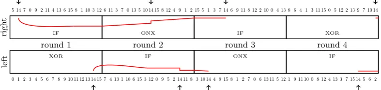
Choosing a message word.

We would like to find the best choice for the single-message word difference

insertion. The

XOR

function located in the 4

th

_{round of right branch must be avoided, so we are looking for a}

message word that is incorporated either very early (so we can propagate the difference backward) or very late

(so we can propagate the difference forward) in this round. Similarly, the

XOR

function located in the 1

st

_round

of left branch must be avoided, so we are looking for a message word that is incorporated either very early (for

a free-start collision attack) or very late (for a semi-free-start collision attack) in this round as well. It is easy to

check that

M

14

is a perfect candidate, being the last inserted in 4

th

round of right branch and the second-to-last

in 1

st

_{round of left branch.}

left

round 1

XOR

0 1 2 3 4 5 6 7 8 9 10 11 12 13 14 15

round 2

IF

7 4 13 1 10 6 15 3 12 0 9 5 2 14 11 8

round 3

ONX

3 10 14 4 9 15 8 1 2 7 0 6 13 11 5 12

round 4

IF

1 9 11 10 0 8 12 4 13 3 7 15 14 5 6 2

righ

t

IF

5 14 7 0 9 2 11 4 13 6 15 8 1 10 3 12

ONX

6 11 3 7 0 13 5 10 14 15 8 12 4 9 1 2

IF

15 5 1 3 7 14 6 9 11 8 12 2 10 0 4 13

XOR

8 6 4 1 3 11 15 0 5 12 2 13 9 7 10 14

Fig. 2.

The shape of our differential path for

RIPEMD-128

. The numbers are the message words inserted at each step and

the red curves represent the rough amount differences in the internal state during each steps. The arrows show where the

bit differences are injected with

M14

.

it might be more interesting to not absorb the difference if it can erase another difference in later steps). We

give the rough skeleton of our differential path in Figure 2. Both differences inserted in the 4

th

_{round of left and}

right branches are simply propagated forward for a few steps and we are very lucky that this linear propagation

leads to two final internal states whose difference can be mutually erased after application of the compression

function finalization and feed-forward (which is yet another argument in favor of

M

14

). All differences inserted in

the 3

rd

and 2

nd

rounds of left and right branches are propagated linearly backward and will be later connected

to the bit difference inserted in the 1

st

round by the non-linear part. Note that since a non-linear part usually

has a low differential probability, we will try to make it as thin as possible. No difference will be present in the

input chaining variable, so the trail is well suited for a semi-free-start collision attack. Following this method and

reusing notations from [4], we eventually obtain the differential path depicted in Figure 5 of Appendix F, the “?”

representing unrestricted bits that will be constrained during the non-linear parts search. We had to choose the bit

position for the message

M

14

difference insertion and among the 32 possible choices, the most significant bit was

selected because it is the one maximizing the differential probability of the linear part we just built (this finds an

explanation by the fact that at the most significant bit position many conditions due to carry control in modular

additions are avoided).

3.3

The non-linear differential part search tool

Our goal starting from Figure 5 of Appendix F is now to instantiate the unconstrained bits denoted by “?” such

that only inactive (“0”, “1” or “-”) or active bits (“n”, “u” or “x”) remain and such that the path contains no

direct inconsistency. This is in general a very complex task, but we implemented a tool similar to [4] for

SHA-1

in

order to perform this task in an automated way. Since

RIPEMD-128

also belongs to the

MD-SHA

family, the original

technique works well, in particular when used in a round with a non-linear boolean function such as

IF.

We have to find one non-linear part in each branch and note that they can be handled independently. We

included the special constraint that the non-linear parts should be as thin as possible (i.e. spreading on the

fewer possible amount of steps), so as to later reduce the overall complexity (linear parts have higher differential

probability than non-linear ones).

3.4

The final differential path skeleton

Applying our non-linear part search tool to the trail given in Figure 5 of Appendix F, we obtain the differential

path in Figure 6 of Appendix F, for which we provide at each step

i

the differential probability P

l

[

i

] and P

r

[

i

] of

left and right branch respectively. Also, we give for each step

i

the accumulated probability P[

i

] starting from last

step, i.e. P[

i

] =

Qj

_j

=

₌₆₃

i

(P

r

[

j

]

·

P

l

[

j

]).

One can check that the trail has differential probability 2

−85

.

09

_(i.e.

Q

63

i

=0

P

l

_[

_i

_{] = 2}

−85

.

09

_{) in the left branch}

and 2

−145

(i.e.

Q

63

i

=0

P

r

_[

_i

_{] = 2}

−145

_{) in the right branch. Its overall differential probability is 2}

−230

.

09

_{and since we}

have 511 bits of message with unspecified value (one bit of

M

4

is already set to “1”), plus 127 unrestricted bits

of chaining variable (one bit of

X

0

=

Y

0

=

h

3

is already set to “0”), we expect many solutions to exist (about

2

407

.

91

_).

In order for the path to provide a collision, the bit difference in

X

61

must erase the one in

Y

64

during the

finalization phase of the compression function:

h

0

₂

=

X

61

Y

64

h

3

. Since the signs of these two bit differences

are not specified, this happens with probability 2

−1

and the overall probability to follow our differential path and

to obtain a collision for a randomly chosen input is 2

−231

.

09

.

4

Utilization of the freedom degrees

can be used to reduce the complexity of the straightforward collision search (i.e. choosing random 512-bit message

values) that requires about 2

231

.

09

_RIPEMD-128

_{step computations. We will utilize these freedom degrees in three}

phases:

•

Phase 1

: we first fix some internal state and message bits in order to prepare the attack. This will allow us

to handle in advance some conditions in the differential path as well as facilitating the merging phase. This

preparation phase is done once for all.

•

Phase 2

: we will fix iteratively the internal state words

X

21

,

X

22

,

X

23

,

X

24

from left branch, and

Y

11

,

Y

12

,

Y

13

,

Y

14

from right branch, as well as message words

M

12

,

M

3

,

M

10

,

M

1

,

M

8

,

M

15

,

M

6

,

M

13

,

M

4

,

M

11

and

M

7

(the ordering is important). This will provide us a starting point for the merging phase and due to a lack

of freedom degrees, we will need to perform this phase several times in order to get enough starting points to

eventually find a solution for the entire differential path.

•

Phase 3

: we use the remaining unrestricted message words

M

0

,

M

2

,

M

5

,

M

9

and

M

14

to efficiently merge the

internal states of the left and right branches.

4.1

Phase 1: preparation

Before starting to fix a lot of message and internal state bit values, we need to prepare the differential path from

Figure 6 of Appendix F so that the merge can later be done efficiently and so that the probabilistic part will not be

too costly. Understanding these constraints requires a deep insight of the differences propagation and conditions

fulfillment inside the

RIPEMD-128

step function. Therefore, the reader not interested in the details of the differential

path construction is advised to skip this subsection.

The first constraint that we set is

Y

3

=

Y

4

. The effect is that the

IF

function at step 4 of the right branch,

IF(

Y

2

, Y

4

, Y

3

) = (

Y

2

∧

Y

3

)

⊕

(

Y

2

∧

Y

4

) =

Y

3

=

Y

4

, will not depend on

Y

2

anymore. We will see in Section 4.3 that

this constraint is crucial in order for the merge to be performed efficiently.

The second constraint is

X

24

=

X

25

(except the two bit positions of

X

24

and

X

25

that contain differences),

and the effect is that the

IF

function at step 26 of the left branch (when computing

X

27

),

IF(

X

26

, X

25

, X

24

) =

(

X

26

∧

X

25

)

⊕

(

X

26

∧

X

24

) =

X

24

=

X

25

, will not depend on

X

26

anymore. Before the final merging phase starts,

we will not know

M

0

, and having this

X

24

=

X

25

constraint will allow us to directly fix the conditions located

on

X

27

without knowing

M

0

(since

X

26

directly depends on

M

0

). Moreover, we fix the 12 first bits of

X

23

and

X

24

to “01000100u001” and “01000011110” respectively because this choice is among the few that minimizes the

number of bits of

M

9

that needs to be set in order to verify many of the conditions located on

X

27

.

The third constraint consists in setting the bits 18 to 30 of

Y

20

to “0000000000000”. The effect is that for

these 13 bit positions, the

ONX

function at step 21 of the right branch (when computing

Y

22

),

ONX(

Y

21

, Y

20

, Y

19

) =

(

Y

21

∨

Y

20

)

⊕

Y

19

, will not depend on the 13 corresponding bits of

Y

21

anymore. Again, because we will not know

M

0

before the merging phase starts, this constraint will allow us to directly fix the conditions on

Y

22

without

knowing

M

0

(since

Y

21

directly depends on

M

0

).

Finally, the last constraint that we enforce is that the first two bits of

Y

22

are set to “10” and the first three

bits of

M

14

are set to “011”. This particular choice of bit values is among the ones that reduces the most the

spectrum of possible carries during the addition of step 24 (when computing

Y

25

) and we obtain a probability

improvement to reach “u” in

Y

25

from 2

−1

to 2

−0

.

25

.

We give in Figure 7 of Appendix F our differential path after having set these constraints (we denote a bit [

X

i]j

with the constraint [

X

i]j

= [

X

i

−1

]j

by “ˆ”). We observe that all the constraints set in this subsection consume

in total 32 + 51 + 13 + 5 = 101 bits of freedom degrees, and a huge amount of solutions (about 2

306

.

91

) are still

expected to exist.

4.2

Phase 2: generating a starting point

Once the differential path properly prepared in phase 1, we would like to utilize the huge amount of freedom degrees

available to fulfill directly as many conditions as possible. Our approach is to fix the value of the internal states

in both the left and right branches (they can be handled independently), exactly in the middle of the non-linear

parts where the number of conditions is important. Then, we will fix the message words one by one following a

particular scheduling, and propagating the bit values forward and backward from the middle of the non-linear

parts in both branches.

Fixing the message words.

Similarly to the internal state words, we randomly fix the value of message words

M

12

,

M

3

,

M

10

,

M

1

,

M

8

,

M

15

,

M

6

,

M

13

,

M

4

,

M

11

and

M

7

(following this particular ordering that facilitates the

convergence towards a solution). The difference here is that the left and right branch computations are no more

independent since the message words are used in both of them. However, this does not change anything to our

algorithm and the very same process is applied: for each new message word randomly fixed, we compute forward

and backward from the known internal state values and check for any inconsistency, using backtracking and reset

if needed.

Overall, finding one new solution for this entire phase 2 takes about 5 minutes of computation on a recent PC

with a naive implementation

4

_{. However, when one starting point is found, we can generate many for a very cheap}

cost by randomizing message words

M

4

,

M

11

and

M

7

since the most difficult part is to fix the 8 first message

words of the schedule. For example, once a solution is found, one can directly generate 2

18

_{new starting points by}

randomizing a certain portion of

M

7

(because

M

7

has no impact on the validity of the non-linear part in the left

branch, while in the right branch one has only to ensure that the last 14 bits of

Y

20

are set to “u0000000000000”)

and this was verified experimentally.

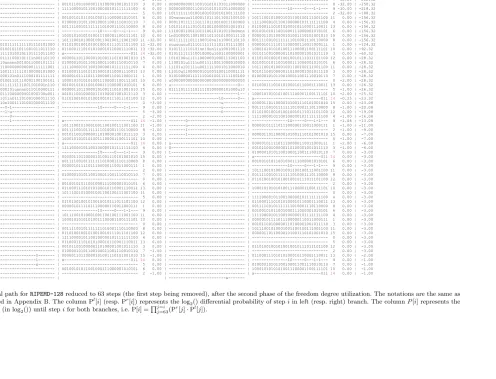
We give an example of such a starting point in Figure 3 and we emphasize that by “solution” or “starting point”

we mean a differential path instance with

exactly

the same probability profile as this one. The 3 constrained bit

values in

M

14

are coming from the preparation in phase 1, and the 3 constrained bit values in

M

9

are necessary

conditions in order to fulfill step 26 when computing

X

27

. It is also important to remark that whatever instance

found during this second phase, the position of these 3 constrained bit values will always be the same thanks to

our preparation in phase 1.

The probabilities displayed in Figure 3 for early steps (steps 0 to 14) are not meaningful here since they assume

an attacker only computing forward, while in our case we will compute backwards from the non-linear parts to

the early steps. However, we can see that the uncontrolled accumulated probability (i.e. step

3

in right side of

Figure 1) is now improved to 2

−29

.

32

, or 2

−30

.

32

if we add the extra condition for the collision to happen at the

end of the

RIPEMD-128

compression function.

4.3

Phase 3: merging left and right branches

At the end of the second phase, we have several starting points equivalent to the one from Figure 3, with many

conditions already verified and an uncontrolled accumulated probability of 2

−30

.

32

_{. Our goal for this third phase is}

now to use remaining free message words

M

0

,

M

2

,

M

5

,

M

9

,

M

14

and make sure that both left and right branches

start with the same chaining variable.

We recall that during the first phase we enforced that

Y

3

=

Y

4

, and for the merge we will require an extra

constraint

X

>>>

5

5

M

4

=

0xffffffff. The message words

M

14

and

M

9

will be utilized to fulfill this constraint, and

message words

M

0

,

M

2

and

M

5

will be used to perform the merge of the two branches only with a few operations,

and with a success probability of 2

−34

.

Handling the extra constraint with

M

14

and

M

9

.

First, let us deal with the constraint

X

5

>>>

5

M

4

=

0xffffffff, which can be rewritten as

X

5

= (0xffffffff

M

4

)

<<<

5

and then

X

9

>>>

11

(

X

8

⊕

X

7⊕

X

6

)

M

8

K

0

l

=

(0xffffffff

M

4

)

<<<

5

by replacing

M

5

using update formula of step 8 in left branch. Finally, isolating

X

6

and

replacing it using update formula of step 9 in left branch we obtain:

M9

=

X

>>>13

10

((

X

9>>>11

M8

K

0l

(

0xffffffff

M4

)

<<<5

)

⊕

X8

⊕

X7

)

K

0l

(

X9

⊕

X8

⊕

X7

)

.

(1)

All values on the right side of this equation are known if

M

14

is fixed. Therefore, so as to fulfill our extra constraint,

what we could do is to simply pick a random value for

M

14

, and then directly deduce the value of

M

9

thanks to

equation (1). However, one can see in Figure 3 that 3 bits are already fixed in

M

9

(the last one being the 10

th

bit

of

M

9

) and thus a valid solution would be found only with probability 2

−3

. In order to avoid this extra complexity

factor, we will first randomly fix the first 24 bits of

M

14

and this will allow us to directly deduce the first 10 bits

of

M

9

that fulfill our extra constraint up to the 10

th

bit (because knowing the first 24 bits of

M

14

will lead to the

first 24 bits of

X

11

,

X

10

,

X

9

,

X

8

and the first 10 bits of

X

7

, which is exactly what we need according to equation

(1)). Once a solution is found after 2

3

tries on average, we can randomize the remaining

M

14

unrestricted bits

(the 8 most significant bits) and eventually deduce the 22 most significant bits of

M

9

with equation (1). With this

method, we completely remove the extra 2

3

factor, because the cost is amortized by the final randomization of the

8 most significant bits of

M

14

.

4

Step X

i

W

li



li

P

l

[i] Y

i

W

ri



ri

P

r

[i] P[i]

-3: --- -2: --- -1: ---

00: ---0--- | --- 0 0.00 | ---0--- | --- 5 -2.00 | -287.32 01: --- | 00000101111011100000110011000111 1 0.00 | ---01--- | x---011 14 -1.00 | -285.32 02: --- | --- 2 0.00 | ---n--- | 01000010101100100011001110010110 7 -32.00 | -284.32 03: --- | 00101100100000110100001001011110 3 0.00 | 00000000001100101010101011000000 | --- 0 -32.00 | -252.32 04: --- | 11110000101100100000101111111100 4 0.00 | 00000000001100101010101011000000 | ---0---1-1--- 9 -31.00 | -220.32 05: --- | --- 5 0.00 | 10111111101001001001010100111100 | --- 2 -32.00 | -189.32 06: --- | 00100101011001000111000001010101 6 0.00 | 00nuuuuuu11000110111011001100100 | 10111001010001001100100111001100 11 0.00 | -157.32 07: --- | 01000010101100100011001110010110 7 0.00 | 00011011111101110110010011100000 | 11110000101100100000101111111100 4 0.00 | -157.32 08: --- | 00111100101111111010001110110000 8 0.00 | 10101101110101010010000001001011 | 01100011101010100010110001110011 13 0.00 | -157.32 09: --- | ---0---1-1--- 9 0.00 | 111000110011011100101010110n0nnn | 00100101011001000111000001010101 6 0.00 | -157.32 10: --- | 10001010101010011100001100111101 10 0.00 | 1n010000110010011011010100011110 | 00000110110000101001110101001010 15 0.00 | -157.32 11: --- | 10111001010001001100100111001100 11 -32.00 | 001111111011100010nu1n1000110110 | 00111100101111111010001110110000 8 0.00 | -157.32 12: 00111010101011111111101110101000 | 01101001001010010010111011101100 12 -32.00 | nuuuuuuu011101111111101101111001 | 00000101111011100000110011000111 1 0.00 | -125.32 13: 01110011001001011011001011011110 | 01100011101010100010110001110011 13 -32.00 | 0101111110101nn10un11u1001001110 | 10001010101010011100001100111101 10 0.00 | -93.32 14: 11110100011110100101101111011100 | x---011 14 -32.00 | 010111111110010000u1001100000001 | 00101100100000110100001001011110 3 0.00 | -61.32 15: 01101010101111000101111n00110110 | 00000110110000101001110101001010 15 0.00 | 1010100u111110000001000111001100 | 01101001001010010010111011101100 12 0.00 | -29.32 16: 01010110010unnnn0010011000101111 | 01000010101100100011001110010110 7 0.00 | 1100101u1111u0011110011000010000 | 00100101011001000111000001010101 6 0.00 | -29.32 17: 0100101n011000000000000111111001 | 11110000101100100000101111111100 4 0.00 | 11101u101111u0011111001011000010 | 10111001010001001100100111001100 11 0.00 | -29.32 18: 10100010110011111110100000101000 | 01100011101010100010110001110011 13 0.00 | 11010u11000000101001100110001111 | 00101100100000110100001001011110 3 0.00 | -29.32 19: 001u10010000101n0111000101111111 | 00000101111011100000110011000111 1 0.00 | 01010000011111101010011111100100 | 01000010101100100011001110010110 7 0.00 | -29.32 20: 01100001101001101110001100100101 | 10001010101010011100001100111101 10 0.00 | u0000000000000000000000000000000 | --- 0 -2.00 | -29.32 21: 1011110100111111111001101001n110 | 00100101011001000111000001010101 6 0.00 | u---0-- | 01100011101010100010110001110011 13 0.00 | -27.32 22: 101110111000101unnnn011010000111 | 00000110110000101001110101001010 15 0.00 | 01111011111011110100000101000u10 | --- 5 -1.00 | -27.32 23: 1011111110111000000001000100u001 | 00101100100000110100001001011110 3 0.00 | ---1-- | 10001010101010011100001100111101 10 -2.00 | -26.32 24: 0100001011011n011101001000011110 | 01101001001010010010111011101100 12 0.00 | ---10---0-- | x---011 14 -0.25 | -24.32 25: 01000010110n10011101001000011110 | --- 0 -3.00 | ---u--- | 00000110110000101001110101001010 15 0.00 | -24.08 26: ---u---0-1--- | ---0---1-1--- 9 -1.00 | ---u--- | 00111100101111111010001110110000 8 -1.00 | -21.08 27: 1---0---1-u--- | --- 5 -3.00 | ---0--- | 01101001001010010010111011101100 12 0.00 | -19.08 28: 0---1---0--- | --- 2 -2.00 | --- | 11110000101100100000101111111100 4 -1.00 | -16.08 29: n---1--- | x---011 14 -1.00 | ---0--- | ---0---1-1--- 9 -1.08 | -13.08 30: u--- | 10111001010001001100100111001100 11 -1.00 | ---u--- | 00000101111011100000110011000111 1 -1.00 | -11.00 31: u--- | 00111100101111111010001110110000 8 -1.00 | ---1--- | --- 2 -1.00 | -9.00 32: 1--- | 00101100100000110100001001011110 3 0.00 | ---1--- | 00000110110000101001110101001010 15 0.00 | -7.00 33: --- | 10001010101010011100001100111101 10 0.00 | --- | --- 5 -1.00 | -7.00 34: --- | x---011 14 0.00 | u--- | 00000101111011100000110011000111 1 -2.00 | -6.00 35: --- | 11110000101100100000101111111100 4 0.00 | 0--- | 00101100100000110100001001011110 3 -1.00 | -4.00 36: --- | ---0---1-1--- 9 0.00 | 1--- | 01000010101100100011001110010110 7 0.00 | -3.00 37: --- | 00000110110000101001110101001010 15 0.00 | --- | x---011 14 0.00 | -3.00 38: --- | 00111100101111111010001110110000 8 0.00 | --- | 00100101011001000111000001010101 6 0.00 | -3.00 39: --- | 00000101111011100000110011000111 1 0.00 | --- | ---0---1-1--- 9 0.00 | -3.00 40: --- | --- 2 0.00 | --- | 10111001010001001100100111001100 11 0.00 | -3.00 41: --- | 01000010101100100011001110010110 7 0.00 | --- | 00111100101111111010001110110000 8 0.00 | -3.00 42: --- | --- 0 0.00 | --- | 01101001001010010010111011101100 12 0.00 | -3.00 43: --- | 00100101011001000111000001010101 6 0.00 | --- | --- 2 0.00 | -3.00 44: --- | 01100011101010100010110001110011 13 0.00 | --- | 10001010101010011100001100111101 10 0.00 | -3.00 45: --- | 10111001010001001100100111001100 11 0.00 | --- | --- 0 0.00 | -3.00 46: --- | --- 5 0.00 | --- | 11110000101100100000101111111100 4 0.00 | -3.00 47: --- | 01101001001010010010111011101100 12 0.00 | --- | 01100011101010100010110001110011 13 0.00 | -3.00 48: --- | 00000101111011100000110011000111 1 0.00 | --- | 00111100101111111010001110110000 8 0.00 | -3.00 49: --- | ---0---1-1--- 9 0.00 | --- | 00100101011001000111000001010101 6 0.00 | -3.00 50: --- | 10111001010001001100100111001100 11 0.00 | --- | 11110000101100100000101111111100 4 0.00 | -3.00 51: --- | 10001010101010011100001100111101 10 0.00 | --- | 00000101111011100000110011000111 1 0.00 | -3.00 52: --- | --- 0 0.00 | --- | 00101100100000110100001001011110 3 0.00 | -3.00 53: --- | 00111100101111111010001110110000 8 0.00 | --- | 10111001010001001100100111001100 11 0.00 | -3.00 54: --- | 01101001001010010010111011101100 12 0.00 | --- | 00000110110000101001110101001010 15 0.00 | -3.00 55: --- | 11110000101100100000101111111100 4 0.00 | --- | --- 0 0.00 | -3.00 56: --- | 01100011101010100010110001110011 13 0.00 | --- | --- 5 0.00 | -3.00 57: --- | 00101100100000110100001001011110 3 0.00 | --- | 01101001001010010010111011101100 12 0.00 | -3.00 58: --- | 01000010101100100011001110010110 7 -1.00 | --- | --- 2 0.00 | -3.00 59: ---0--- | 00000110110000101001110101001010 15 -1.00 | --- | 01100011101010100010110001110011 13 0.00 | -2.00 60: ---1--- | x---011 14 0.00 | --- | ---0---1-1--- 9 0.00 | -1.00 61: ---x--- | --- 5 0.00 | --- | 01000010101100100011001110010110 7 0.00 | -1.00 62: --- | 00100101011001000111000001010101 6 0.00 | --- | 10001010101010011100001100111101 10 0.00 | -1.00 63: --- | --- 2 -1.00 | --- | x---011 14 0.00 | -1.00 64: --- | | ---x---

Fig. 3.

The differential path for

RIPEMD-128

, after the second phase of the freedom degree utilization. The notations are the same as in [4] and are described in Appendix B. The column

P

l

_[

_i

_{] (resp. P}

r

_[

_i

_{]) represents the log}

2

() differential probability of step

i

in left (resp. right) branch. The column

P

[

i

] represents the cumulated probability (in log

2

()) until step

i

for both

branches, i.e. P[

i

] =

Q

j=i

j=63

(P

r

Merging the branches with

M

0

,

M

2

and

M

5

.

Once

M

9

and

M

14

fixed, we still have message words

M

0

,

M2

and

M

5

to determine for the merging. One can see that with only these three message words undetermined,

all internal state values except

X

2

,

X

1

,

X

0

,

X

−1

,

X

−2

,

X

−3

and

Y

2

,

Y

1

,

Y

0

,

Y

−1

,

Y

−2

,

Y

−3

are fully known when

computing backwards from the non-linear parts in each branch.

This is where our first constraint

Y

3

=

Y

4

comes into play. Indeed, when writing

Y

1

from the equation from

step 4 in right branch, we have:

Y

1

=

Y

5

>>>

13

(

Y

4

∧

Y

2

⊕

Y

3

∧

Y

2

)

M

9

K

0

r

=

Y

5

>>>

13

Y

3

M

9

K

0

r

which means that

Y

1

is already completely determined at this point (the bit condition present in

Y

1

in Figure 3

is actually handled for free when fixing

M

14

and

M

9

, since it requires to know the 9 first bits of

M

9

). In other

words, the constraint

Y

3

=

Y

4

allowed

Y

1

to not depend on

Y

2

which is currently undetermined. Another effect of

this constraint can be seen when writing

Y

2

from the equation from step 5 in right branch:

Y

2

=

Y

6

>>>

15

(

Y

5

∧

Y

3

⊕

Y

4

∧

Y

3

)

M2

K

0

r

=

Y

>>>

15

6

(

Y

5

∧

Y

3

)

M2

K

0

r

=

C

0

M2

where

C

0

=

Y

6

>>>

15

(

Y

5

∧

Y

3

)

K

0

r

is a constant.

Our second constraint

X

>>>

5

5

M

4

=

0xffffffff

is useful when writing

X

1

and

X

2

from the equations from

step 4 and 5 in left branch

X2

=

X

6>>>8

(

X5

⊕

X4

⊕

X3

)

M

5

=

C1

M

5

X1

=

X

>>>5

5

(

X4

⊕

X3

⊕

X2

)

M4

=

0xffffffff

(

X4

⊕

X3

⊕

X2

) =

X4

⊕

X3

⊕

X2

=

X4

⊕

X3

⊕

(

C1

M

5

)

where

C

1

=

X

6

>>>

8

(

X

5

⊕

X

4

⊕

X

3

) is a constant.

Finally, our ultimate goal for the merge is to ensure that

X

−3

=

Y

−3

,

X

−2

=

Y

−2

,

X

−1

=

Y

−1

and

X

0

=

Y

0

,

knowing that all other internal states are determined when computing backwards from the non-linear parts in each

branch, except

Y

2

=

C

0

M2

,

X

2

=

C

1

M

5

and

X

1

=

X

4

⊕

X

3

⊕

(

C

1

M

5). We therefore write the equations

relating these eight internal state words:

X0

=

X

>>>12

4

(

X3

⊕

X2

⊕

X1

)

M3

=

X

>>>12

4

X4

M3

=

Y0

=

Y

>>>11

4

(

Y3

∧

Y1

⊕

Y2

∧

Y1

)

M

0

K

0r

=

Y

>>>11

4

(

Y3

∧

Y1

⊕

(

C0

M

2

)

∧

Y1

)

M

0

K

0r

X

−1

=

X

3>>>15

(

X2

⊕

X1

⊕

X0

)

M

2

=

X

3>>>15

(

X4

⊕

X3

⊕

X0

)

M

2

=

Y

−1

=

Y

3>>>9

(

Y2

∧

Y0

⊕

Y1

∧

Y0

)

M7

K

r

0

=

Y

>>>9

3

((

C0

M

2

)

∧

X0

⊕

Y1

∧

X0

)

M7

K

0r

X

−2

=

X

2>>>14

(

X1

⊕

X0

⊕

X

−1

)

M1

= (

C1

M

5

)

>>>14

(

X4

⊕

X3

⊕

(

C1

M

5

)

⊕

X0

⊕

X

−1

)

M1

=

Y

−2

=

Y

2>>>9

(

Y1

∧

Y

−1

⊕

Y0

∧

Y

−1

)

M14

K

0r

= (

C0

M

2

)

>>>9

(

Y1

∧

X

−1

⊕

X0

∧

X

−1

)

M14

K

r0

X

−3

=

X

1>>>11

(

X0

⊕

X

−1

⊕

X

−2

)

M

0

= (

X4

⊕

X3

⊕

(

C1

M

5

))

>>>11

(

X0

⊕

X

−1

⊕

X

−2

)

M

0

=

Y

−3

=

Y

1>>>8

(

Y0

∧

Y

−2

⊕

Y

−1

∧

Y

−2

)

M

5

K

0r

=

Y

>>>8

1

(

X0

∧

X

−2

⊕

X

−1

∧

X

−2

)

M

5

K

0r

If these four equations are verified, then we have merged left and right branch to the same input chaining

variable. We first remark that

X

0

is already fully determined and thus the second equation

X

−1

=

Y

−1

only

depends on

M2

. Moreover, it is a T-function in

M2

(any bit

i

of the equation depends only on the

i

first bits of

M2

) and can therefore be solved very efficiently bit per bit. We give in Appendix C more details on how to solve

this T-function and our average cost in order to find one

M2

solution is one

RIPEMD-128

step computations.

Since

X

0

is already fully determined, from the

M2

solution previously obtained we directly deduce the value of

M

0

to satisfy the first equation

X

0

=

Y

0

. From

M2

we can compute the value of

Y

−2

and we know that

X

−2

=

Y

−2

and we calculate

X

−3

from

M

0

and

X

−2

. At this point, the two first equations are fulfilled and we still have the

value of

M

5

to choose.

The third equation can be rewritten

V

>>>

14

_{= (}

_V

_⊕

_C

2

)

C

3

, where

V

=

X

[2] = (

C

1

M

5) and

C

2

,

C

3

are two

constants. Similarly, the fourth equation can be rewritten

V

>>>

11

_{= (}

_V

C

4

)

⊕

C

5

, where

C

4

,

C

5

are two constants.

Solving either of these two equations with regards to

V

can be costly because of the rotations, so we combine them

to create simpler one: ((

V

⊕

C

2

)

C

3

)

<<<

3

= (

V

C

4

)

⊕

C

5

. This equation is easier to handle because the rotation

coefficient is small: we guess the 3 most significant bits of ((

V

⊕

C

2

)

C

3

) and we solve simply the equation 3-bit

layer per 3-bit layer, starting from the least significant bit. From the value of

V

deduced, we straightforwardly

obtain

M

5

=

C

1

V

and the cost of recovering

M

5

is equivalent to 8

RIPEMD-128

step computations (the 3-bit

guess implies a factor of 8, but the resolution can be implemented very efficiently with tables).

fourth equations will be fulfilled. Moreover, one can check in Figure 3 that there is one bit condition on

X

0

=

Y

0

and one bit condition on

Y

2

and this further adds up a factor 2

−2

. We evaluate the whole process to cost about

19

RIPEMD-128

step computations on average: there are 17 steps to compute backwards after having identified a

proper couple

M

14

,

M

9

, and the 8

RIPEMD-128

step computations to obtain

M

5

are only done 1

/

4 of the time

because the two bit conditions on

Y

2

and

X

0

=

Y

0

are filtered before.

To summarize the merging: we first compute a couple

M

14

,

M

9

that satisfies a special constraint, we find a

value of

M

2

that verifies

X

−1

=

Y

−1

, then we directly deduce

M

0

to fulfill

X

0

=

Y

0

, and we finally obtain

M

5

to satisfy a combination of

X

−2

=

Y

−2

and

X

−3

=

Y

−3

. Overall, with only 19

RIPEMD-128

step computations on

average, we were able to do the merging of the two branches with probability 2

−34

.

5

Results and implementation

5.1

Complexity analysis and implementation

After the quite technical description of the attack in previous section, we would like to rewrap everything to get

a clearer view of the attack complexity, the amount of freedom degrees etc. Given a starting point from phase

2, the attacker can perform 2

26

merge processes (because 3 bits are already fixed in both

M

9

and

M

14

, and the

extra constraint consumes 32 bits) and since one merge process succeeds only with probability of 2

−34

, he obtains

a solution with probability 2

−8

. Since he needs 2

30

.

32

solutions from the merge to have a good chance to verify the

probabilistic part of the differential path, a total of 2

38

.

32

_{starting points will have to be generated and handled.}

The attack starts at the end of phase 1, with the path from Figure 7 of Appendix F. From here, he generates

2

38

.

32

_{starting points in phase 2, that is 2}

38

.

32

_{differential paths like the one from Figure 3 (with the same step}

probabilities). For each of them, in phase 3 he tries 2

26

times to find a solution for the merge with an average

complexity of 19

RIPEMD-128

step computations for each try. The semi-free-start collision final complexity is 19

·

2

26+38

.

32

RIPEMD-128

step computations, which corresponds to (19

/

128)

·

2

64

.

32

= 2

61

.

57

RIPEMD-128

compression

function computations (there are 64 steps computations in each branch).

The merge process has been implemented and we give in Appendix D an example of a message and chaining

variable couple that verifies the merge (i.e. they follow the differential path from Figure 6 of Appendix F until

step 25 of the left branch and step 20 of the right branch). We measured the efficiency of our implementation in

order to confront it to our theoretic complexity estimation. As point of reference, we observed that on the same

computer, an optimized implementation of

RIPEMD-160

(OpenSSL v.1.0.1c) performs 2

21

.

44

_{compression function}

computations per second. With 4 rounds instead of 5 and about 3

/

4 less operations per step, we extrapolated

that

RIPEMD-128

would perform at 2

22

.

17

compression function computations per second. Our implementation

performs 2

24

.

61

merge process (both phase 2 and phase 3) per second on average, which therefore corresponds

to a semi-free-start collision final complexity of 2

61

.

88

RIPEMD-128

compression function computations. While our

practical results confirm our theoretical estimations, we emphasize that the latter are a bit pessimistic, since our

attack implementation is not really optimized. As a side note, we also verified experimentally that the probabilistic

part in both left and right branch can be fulfilled.

A last point needs to be checked: the complexity estimation for the generation of the starting points. Indeed, as

much as 2

38

.

32

_{starting points are required at the end of phase 2 and the algorithm being quite heuristic, it is hard}

to analyze precisely. The amount of freedom degrees is not an issue since we already saw in Section 4.1 that about

2

306

.

91

solutions are expected to exist for the differential path at the end of phase 1. A completely new starting

point takes about 5 minutes to be outputted on average with our implementation, but from one such path we can

directly generate 2

18

equivalent ones by randomizing

M

7

. Using the OpenSSL implementation as reference, this

amounts to 2

50

.

72

RIPEMD-128

computations to generate all the starting points that we need in order to find a

semi-free-start collision. This gross estimation is extremely pessimistic since its doesn’t even take in account the fact

that once a starting point is found, one can also randomize

M

4

and

M

11

to find many other valid candidates with

a few operations. Finally, one may argue that with this method the starting points generated are not independent

enough (in backward direction when merging and/or in forward direction for verifying probabilistically the linear

part of the differential path). However, no such correlation was detected during our experiments and previous

attacks on similar hash functions [13, 14] showed that only a few rounds were enough to observe independence

between bit conditions. In addition, even if some correlations existed, since we are looking for many solutions, the

effect would be averaged among good and bad candidates.

5.2

Collision for the

RIPEMD-128

compression function