VOLUME 37, ARTICLE 15, PAGES 455
,
492
PUBLISHED 22 AUGUST 2017
http://www.demographic-research.org/Volumes/Vol37/15/ DOI: 10.4054/DemRes.2017.37.15
Research Article
Does socioeconomic status matter?
The fertility transition in a northern Italian
village (marriage cohorts 1900‒1940)
Rosella Rettaroli
Alessandra Samoggia
Francesco Scalone
© 2017 Rettaroli, Samoggia & Scalone.
This open-access work is published under the terms of the Creative Commons Attribution NonCommercial License 2.0 Germany, which permits use, reproduction, and distribution in any medium for noncommercial purposes, provided the original author(s) and source are given credit.
1 Adding a piece of the puzzle of Italian fertility transition 456
2 Fertility decline and socioeconomic status 457
3 Reproductive differences in the Italian sharecropping system 461
4 The area 462
5 Data sources 465
6 The fertility transition in Granarolo and SES differentials 467
6.1 Main indicators of reproduction and SES 467
6.2 Event history analysis of birth intervals 473
7 Final remarks 481
Does socioeconomic status matter? The fertility transition in a
northern Italian village (marriage cohorts 1900‒1940)
Rosella Rettaroli1
Alessandra Samoggia2
Francesco Scalone2
BACKGROUND
The paper explores the mechanisms of the European fertility transition in northern Italy by social group.
OBJECTIVE
Our objective is to understand when and in which sectors of a rural society the reduction of family size began. We focus on Emilia-Romagna, a region that in the 1990s had the lowest fertility level in Italy. The core purpose of this paper is the analysis of socioeconomic status (SES) fertility differentials, especially between rural sharecroppers and landless rural workers, as well as other non-agricultural groups. METHODS
Our analysis focuses on the reproductive histories of marriage cohorts in the years 1900‒1940. We perform a micro-level statistical analysis of legitimate births of parity 1+.
RESULTS
In this period fertility decline has just begun, and shows a strong decline in the post-WWI marriage cohorts. Although nonagricultural groups lead the downward trend in family size, the role of socioeconomic status means that the path of sharecropper households is atypical.
CONCLUSIONS
The fertility transition proceeds by means of spacing and stopping, testifying to a new attitude towards birth control, which agricultural and nonagricultural social groups adopted in different ways. Usually, the decline in fertility progresses from nonagricultural to rural classes. In the rural world the path is inverted, going from the lower to the upper groups.
CONTRIBUTION
The paper contributes to the debate on the links between socioeconomic status and fertility transition in Italy. It shows that the link between household economy and control of fertility is specific to SES groups, which can follow atypical paths, compared to the known reference model. The use of microdemographic data provides evidence for the hypothesis that the fertility transition can be shaped by the specific social and economic characteristics of population subgroups.
1. Adding a piece of the puzzle of Italian fertility transition
3Although demographic changes in Italy followed the general pattern of demographic transformation in other European countries, downward fertility started later, with the declines in different regions progressing on unusual paths. Even before the demographic transition the Italian reproductive regime presented significant geographical and social differences. National and subnational aggregative studies on Italian fertility decline have shown that the path and the pace of transition can differ considerably between northern and southern regions. The differences can also be much more intensive within the same region, and explanations mostly refer to the socioeconomic structures of the different areas and the ways in which the different population subgroups experienced downward fertility (Santini 2008; Breschi, Pozzi, and Rettaroli 1994; Breschi et al. 2009, 2010, 2014; Del Panta et al. 1996; Del Panta and Scalone 2002; Dalla Zuanna, Rosina, and Rossi 2004; Ge Rondi, Manfredini, and Rettaroli 2008; Santini and Salvini 2007).
It is therefore interesting to study more thoroughly the socioeconomic reproductive differences in the initial phase of the fertility transition. Our aim is to highlight some
key points of the fertility decline in the first decades of the 20th century in Granarolo, a
north Italian village, using a micro-longitudinal approach and considering socioeconomic status (SES). The case study of Granarolo has significant features which are of interest both historically and theoretically. While in other areas of Italy the steady
decline in marital fertility began in the last decade of the 19th century, in the
Emilia-Romagna region where Granarolo is situated it happened later, roughly during the period 1911‒1921 (Livi Bacci 1977). This was probably due to the relatively high mortality level and to the late economic development of the area, with respect to the
national context.4 The economic immobility of this area resulted in the persistence of
traditional forms of land management, as shown by the presence of numerous sharecropping households, which needed large families and children to employ in agricultural work. The land in Granarolo was shared by two different kinds of agricultural worker, the sharecroppers, who had the highest fertility level, and landless labourers, who had the lowest fertility level. These two social groups lived among other smaller, nonagricultural social classes, some of them traditionally considered forerunners in the fertility decline – typically, in the preindustrial age, rural groups lived in the same villages as more modern and progressive social actors. These characteristics enable a twofold objective: to detect the timing of the fertility decline and to highlight the changes in fertility models by SES and marriage cohort. Analysing the role of socioeconomic status during the transition allows us to reconstruct the fertility path and the structure that links the pretransitional and transitional phases. It is of great interest to understand whether the economic and social transformations that occurred during the period under study slowed down the speed of the fertility transition for sharecroppers, who enjoyed greater material stability than the other rural groups, which were more vulnerable to the economic climate. In the social context of Granarolo there were present social classes with lower fertility such as professionals and skilled workers, which should have acted as forerunners in new fertility behaviours and had already begun to control the size of their families.
In the next section of this paper we briefly review the main studies of historical fertility decline that focus on the role of socioeconomic factors. In sections 3 and 4 we describe the socioeconomic characteristics of the study area and show how the Italian sharecropping system shaped the reproductive behaviour that conditioned the fertility transition in the area. In section 5, sources of data are presented, and the results from both aggregate and micro-level analysis are presented and discussed in section 6.
2. Fertility decline and socioeconomic status
The existing literature shows that the complex mechanisms behind the shaping and timing of the fertility transition in Western countries are still not completely understood, and it is not yet possible to fill the gaps in the history of the generations (Van Bavel 2004; Reher and Sanz-Gimeno 2007). There are many theories and generalisations of empirical evidence concerning the historical passage from high to low fertility, offering many possible explanatory factors. However, population analysts
4 After National Unification (1861), part of the Emilia-Romagna region belonged to the Papal State, whose
do not agree on the relative weight of these different factors. Some previous studies, mainly based on aggregate data, show the relevance of economic development and industrialization (among others: Davis 1945; Notestein 1945; Carlsson 1966; Galloway, Hammel, and Lee 1994), or stress the importance of the increase in child survival (Easterlin 1996; Reher 2004). Others highlight the role that changes in individual ideational values played with respect to family and household formation and fertility (Lesthaeghe 1977; Lesthaeghe and Wilson 1986; Cleland and Wilson 1987).
The decline in infant and child mortality is supposed to have exerted a huge influence on fertility decline (Preston 1978), even if, in some cases, the empirical evidence has not quantified a strong relation between the two variables (Galloway, Lee, and Hammel 1998; Oris 1995; Dyson 2010; Bengtsson and Ohlsson 1994; Perrenoud and Bourdelais 1998). Other studies show that the mortality decrease is often not great enough to account for the entire fertility decline (Haines 1998; Doepke 2005), and sometimes decreasing infant mortality and fertility reduction are strongly lagged.
In the passage from natural to controlled fertility the demand for children is one of the crucial elements that has to be taken into account (Easterlin 1975; Becker 1981; Caldwell 1982; Easterlin and Crimmins 1985; Galloway, Hammel, and Lee 1994; Dribe 2009; Dribe and Scalone 2014). From an economic point of view, this demand is determined by the advantages or disadvantages of having another child. Advantages derive both from children’s contribution to the family economy and from the support they provide to their parents in old age (Easterlin 1975). Measured in relation to family income, the disadvantages of having children depend on the cost of rearing them, compared to the cost of all of the other goods parents want to possess. According to this supply‒demand point of view, the demand for children can be defined as the number of children a couple wants if no costs are involved in fertility limitation (Easterlin and Crimmins 1985).
Over time, other social factors responsible for downward fertility have emerged, such as the diffusion of mass education. Compulsory primary education increased the cost of rearing children, while the prohibition of child labour became another crucial factor in explaining fertility evolution (Becker 1981; Caldwell 1982; Friedlander 1983; Easterlin and Crimmins 1985).
attitudes and enabled couples to make more rational choices (McLaren 1990; Carter 2001). Thus, marriage fertility adjusted to new circumstances (Cleland 2001; Palloni 2001; Van Bavel 2004).
The joint action of adjustment and innovation is also considered by Coale (1973). For fertility to decline, three conditions are necessary: People must be ready, willing, and able to change their fertility behaviours radically. Readiness refers to the fact that the new target family size must be advantageous to the couple in terms of a cost-benefit evaluation. Willingness is about the acceptability (ethical, moral, religious, etc.) of the new pattern of action and refers to the effort to overcome social pressure, moral objections, and traditional norms. Despite the fact that some past populations had contraceptive methods for limiting their fertility, they were not ready to adopt new behaviours that were against common cultural norms. Lastly, ability refers to the accessibility of the new techniques that are essential for the adoption of new behaviours (Lesthaeghe and Vanderhoeft 2001).
Most of these elements are undoubtedly stratified socioeconomically and are connected to the SES of individuals and households. In the past, elite groups had higher fertility levels than those of lower SES, probably due to their higher infant survival and higher marital fertility (Tsuya et al. 2010). During the transition, or even before, this positive relationship reversed, as observed, for example, in Italy (Livi Bacci 1986;
Skirbekk 2008).5 Higher status groups are the first to invest in child quality because a
higher level of education is linked to rewarding occupations and higher social status. A smaller number of highly educated children also means that the children will be more socially mobile (Van Bavel 2006; Van Bavel et al. 2011). Elite groups are more open culturally and more likely to adopt new emerging attitudes towards procreation, as shown by the processes of secularisation and individualisation (Goldscheider 2006; Lesthaeghe and Surkyn 1988; Norris and Inglehart 2004; Surkyn and Lesthaeghe 2004; Peri-Rotem 2016). Higher status groups represent a vanguard in changing family and fertility behaviours and act as forerunners in the fertility decline (Livi Bacci 1986;
Haines 1992; Dribe and Scalone 2014; Dribe, Oris, and Pozzi 2014).6 The motivation of
forerunners in the fertility decline may be to retain acquired social status and avoid downward mobility, and, for landowners, the changed rules of land inheritance (Bengtsson and Dribe 2014). In several preindustrial Italian communities the intention to avoid the dispersion of family wealth has been shown to be behind urban and rural
5 In pretransitional Sicily (Schneider and Schneider 1996), in the French town of Rouen (Bardet 1983), in England and France (Cummins 2009), in the United States (Jones and Terlit 2008), where the higher social groups start the fertility decline before other groups with a lower socioeconomic status, and everywhere before agricultural families (Haines 1992).
social elites acting as forerunners in the fertility decline (Livi Bacci 1986; Kertzer and Hogan 1989; Viazzo 1989; Breschi et al. 2010).
Some studies point out that at the beginning of the transition, fertility SES differentials increased due to greater individual aspiration, economic opportunity, returns on education, and access to information. Only later did a new, rational attitude towards procreation and changed norms concerning fertility regulation spread to the rest of the population through a diffusion process, along with the narrowing of class differentials (Coale 1967, 1969; Lesthaeghe and Wilson 1986). It is also important to underline that even in the central phases of industrialisation, children’s role in the family strongly differs between SES groups. For elite groups, the demand for children competes with other material family aspirations, while for lower classes and rural families, children still represent an asset for household economic resources.
Blended theory (Cleland 2001; Casterline 2001) proposes that the adoption of fertility control may be due not only to structural changes but also to diffusion processes. Thus, elite groups may act as forerunners because they have easier access to communication channels that enable them to learn new behaviours, new reproductive norms, and new practices earlier than other social classes. Other authors have highlighted that, besides SES differentials, differences in the social interaction of individuals and couples can help to explain the diffusion of new fertility behaviours (Bongaarts and Watkins 1996; Watkins 1990). In particular, Bras shows that during the Dutch fertility transition “couples that had networks containing siblings (in-law) and/or age peers, and people from urban backgrounds, practiced significantly more fertility control” (2014: 177). Some researches of current fertility determinants show that peers are the main source of social learning as they share the same socioeconomic contextual conditions, which are often different from those of previous generations (Bernardi 2003; Rossier and Bernardi 2009), while in the past patriarchal families, parents, who controlled family resources, represented the preferred channel for the dissemination of normative behaviour.
The very few microanalyses on Italy have shown that during the first decades of
the 19th century the upper classes and the bourgeoisie (Salvini 1990) acted as
forerunners in fertility decline (Livi Bacci 1986). Based on the microdata of some rural
communities in Northern and Central Italy in the 19th century, recent studies also
clearly show that, household organisation and family structure could shape the reproductive behaviours of couples even before the fertility decline and the diffusion of contraceptive techniques (Breschi, Manfredini, and Rettaroli 2000; Breschi et al. 2010; Kertzer and Hogan 1989; Rettaroli and Scalone 2012; Quaranta 2011).
(Pizzetti, Fornasin, and Manfredini 2012; Rettaroli and Scalone 2009). Breschi et al. (2014) observe this kind of relationship in an urban context in the 1930s.
3. Reproductive differences in the Italian sharecropping system
In many northern and central areas of Italy, such as Emilia-Romagna, two family
systems coexisted until the middle of the 20th century (Poni 1983), that of sharecroppers
and that of landless labourers, shaping the reproductive system in different ways. In the sharecropping system the landowner entered into a formal contract with the head of the sharecropping family for the full-time employment of all adult members of the household. Sharecroppers lived in a farmhouse on the landowner’s property that was often quite large. These families were largely self-sufficient as they produced their own food and wine and some clothing materials. The sharecroppers were the wealthy rural workers, since landless labourers lived in very poor conditions (Gattamorta 1931).
Although the sharecropper signed a one-year contract7 the landowner had absolute
control over the administration of the farm, and his authority often extended to the private affairs of the sharecropping family (Giorgetti 1974; Sereni 1968). The contract bound all members of the household to work on the farm: They could not work even
one day elsewhere without the owner’s approval (Poni 1977; Sereni 1968).8 The greater
the number of persons who worked the land, the larger farm they could get, and the bigger the possible production and benefit they experienced. Therefore, during most of the life cycle, sharecroppers lived in large extended household or multiple households, in which two or three generations coexisted.
When the workforce of the household was insufficient, the sharecropper could employ a landless labourer. Landless labourers were employed on a daily-wage basis during periods when their work was needed. No contracts existed for this kind of rural labourer, and oral agreements could change with each transaction. Therefore the existence of most day labourers was precarious (Preti 1955; Medici and Orlando 1952), and they had to find accommodation for their families in the few poor houses scattered in the countryside (Tanari 1881). Work was assigned on an individual basis, without
7 However, the most productive sharecropping families stayed longer on the same farm (Tanari 1881).
8 Landowners were always interested in the demographics of sharecropping households. When choosing a
involving the family or domestic unit, who generally did not live on the farm. The labourers’ families neither became large families nor featured the command pyramid structure typical of the sharecropper’s household.
Previous research on the decline of fertility in the Emilia-Romagna region has already shown that sharecropper families had the highest fertility until roughly the end
of the 19th century (Rettaroli and Scalone 2012; Kertzer and Hogan 1989; Breschi et al.
2010). Following the supply-demand and innovation-adjustment schemas, and given the general context of declining fertility due to the onset of the demographic transition, we expect that sharecroppers’ fertility decline started later or progressed slower than that of other rural and nonrural workers. Effectively, the particular provisions of sharecroppers’ contracts rewarded high fertility, since children represented an asset to households given their role of performing light agricultural tasks at very young ages (Kertzer and Hogan 1989; Rettaroli and Scalone 2009, 2012). Since land access was determined by the availability of human capital and was managed under temporary contracts, households with a large number of working-age males with solid farming experience were in a better position to get the best and largest farms to cultivate (Doveri 2000). This is the reason the demand for children, who constituted the future household workforce, was a pressing and vital issue for sharecroppers. Here the Easterlin‒ Crimmins theory of fertility (1985) could look for confirmation: Socioeconomic factors can affect reproductive behaviours, influencing the demand for and supply of children as well as the cost of fertility control. It is therefore possible to hypothesize that in sharecroppers’ households the relative cost of children was lower, thus leading to higher demand. In the first phases of transition, sharecroppers’ unchanged economic circumstances did not demand any “adjustment” (Carlsson 1966), or, according to Coale’s (1973) framework, willingness and readiness were less imperative.
4. The area
Figure 1: Geographical position of Emilia-Romagna and Bologna
The Emilia-Romagna region has for centuries been the natural crossing point for people travelling between southern and northern Italy and between east and west. This privileged position has made the area an important centre of commerce and manufacturing. Granarolo was a traditional rural village with close economic ties to the
city of Bologna.9
However, the city of Bologna did not take part in the rapid industrialization
process of the last decades of the 19th century that involved Europe and other northern
Italian cities. Before National Unification (1861) the area was part of the Papal States, whose economic policy was mainly characterized by high customs duties and scarce circulating capital, and where transport was difficult. Bologna's main economic engine is still agriculture, accompanied by some craft activity and the presence of a very few local industries that have survived the strong national and foreign competition.
The agrarian crisis of the 1880s hindered the process of modernization in Bologna and its hinterland. The commercial policy introduced by the agricultural protectionism of 1887 only benefitted the large landowners and agricultural tenants. Small farms struggled to find an autonomous space in the market and the agricultural proletariat progressively incorporated former settlers, sharecroppers, and small farmers who were impoverished by the crisis and forced to join the landless rural labourers. The excess supply of landless rural labourers led to periodic unemployment and the gradual depreciation of workers in the labour market, as witnessed by the great strikes of the
agricultural proletariat in the early years of the 20th century (Kertzer and Hogan 1989).
It was only at the end of the first decades of the 20thcentury that Bologna and its
hinterland were transformed by the socioeconomic processes of urbanisation, the
beginnings of industrialisation, and the development of large-scale capitalist agriculture on the plains to the northeast of the city (Cazzola 1996). However, important contingents of traditional sharecroppers remained in the southern hilly area and in the northern lowland area bordering the city (Kertzer and Hogan 1989).
During the observational period, agriculture still represented the main economic
activity of the Granarolo population. At the beginning of the 20th century (1911 census),
more than 67% of the working population was employed in the agricultural sector, nearly three-quarters of them farmers and sharecroppers. In the middle of the century (1951 census) agriculture was still a crucial sector employing 63% of workers, while less than 20% worked in industry and manufacturing. Despite its proximity to Bologna, Granarolo was barely involved in the urbanisation process, and 80% of its population still lived in scattered houses according to the 1936 census. Only later did the agglomerated population start to increase, reaching 40% in the 1951 census.
Granarolo has always maintained strong relations with the city, exchanging goods
and people.10 A substantial amount of the agricultural and craft products was directed at
the urban market. Those who could not find employment in agriculture moved to the city, mainly to become apprentices or servants (Bellettini 1971). The subordinate role of
this rural area to the city remained almost unchanged until the mid-20th century, when
the process of urbanisation began to spread (Scalone and Del Panta 2008).11
During the first half of the 20th century the population of Granarolo grew more
slowly than the other municipalities around Bologna. The village showed a small increase in the first two decades, was steady at about 5,000 inhabitants until 1931, and decreased slightly thereafter.
Detailed information on the living standards of the rural population in Italy can be
found in two national surveys, the Jacini Survey (Jacini 1882)12 and the Survey on the
Living Conditions of Italian Farmers13 (Confederazione nazionale dei sindacati fascisti
dell’agricoltura 1930). The two reports show clearly that the living conditions of farmers/sharecroppers and landless labourers were very different: food, housing, and
10 The root word of Granarolo means ‘granary’, underlining the ancient role of the village as Bologna’s granary.
11 Ancient walls enclosed Bologna, which represented a separation from the rural hinterland not only symbolically but also administratively and materially. For centuries, the town gates were locked at night, and customs officers strictly controlled people and goods travelling from the countryside to the town. The separation between Bologna and the countryside gradually weakened over time, and at the beginning of the 20th century the ancient walls were torn down.
12 In 1877 the Italian Government commissioned the Jacini survey (Jacini 1882), which was the most complete and detailed study of Italian agriculture at that time. The survey was sent to municipalities, which reported on agrarian property, cultivation methods, and living conditions in the rural populations. The information was collected from 1877‒1879 and edited by Luigi Tanari (1881).
clothing were quite good for the former and significantly worse for the latter (Tanari 1881; Confederazione nazionale dei sindacati fascisti dell’agricoltura 1930).
Education was compulsory and there were enough schools; but school attendance was insufficient, given that parents frequently needed children to help with agricultural work. As a consequence, illiteracy in Granarolo was always higher than in Bologna: 25.7% (21.6% for males, 30.3% for females) in the 1911 census, and 8.7% (5.9% for males, 11.4% for females) in the 1931 census.
In the first half of the 20th century, Emilia-Romagna experienced a remarkable
increase in life expectancy at birth: It grew from 43 years for both genders in 1901 to 68 years in 1951. In the same period, infant mortality showed a steady decline, which was particularly due to a decrease in neonatal mortality (Pozzi 2000). The infant mortality rate declined from 168 per 1,000 in 1881‒1920 to 96 per 1,000 in 1921‒1940, reaching a level that was lower than either regional or national average (Scalone et al. 2013).
5. Data sources
The data used here is based on the village population register (Anagrafe). The register contains information on all of the households of Granarolo, including the names and family names of household members and their professions, paternity and maternity, dates of birth, death, and marriage, and movements into and/or out of the household. After registering each new family on a new file card, municipality officers continuously noted any possible changes and registered when each event occurred. Each year, newborn or immigrant family members were included, while deceased or emigrated individuals were deleted.
To adjust possible under-recording, mainly of deaths of newborn infants, we checked the village population registers against the civil birth and death registers. The reconstitution of the family cards made it possible to reconstruct all individual and female reproductive histories. We know the dates of childbirths and of all the women at risk of giving birth in any given year, with considerable precision.
observation.14 We grouped the marriage cohorts in four groups of 10 years each. The
first group represents fertility histories that start in the pre-World War I period and are the reference category, while the second group concerns couples formed immediately before and during World War I. The third group comprises marriages that took place in a period of great change: post-war reconstruction, industrialisation, expansion of the urban area of Bologna, and the pro-fertility policy of the Fascist Regime. The fascist pro-fertility policies were still in force for the last marriage cohort group.
Based on this data, the reproductive life histories of 1,505 women were reconstituted and 3,732 births were observed. We also used an additional survey on women’s fertility, carried out with the 1931 census (Istituto Centrale di Statistica del Regno d’Italia 1937), which reported the number of dead and surviving children for all women living in Granarolo at the time of census. Thanks to this information and the availability of vital event registers, for the first two decades we could check the reproductive lives that we had identified using the population register information.
To focus on socioeconomic differentials we classified work activities in occupational groups. At the household level, we take into account the SES of the
household head, based on his reported profession in the population register.15
We chose to classify occupation in four broad groups, following the coding system that Bellettini (1971) proposed in his in-depth study of the rural population of Bologna
in the mid-19th century. The first two groups refer to agricultural occupations and the
last two to non-agricultural occupations. We linked this coding to the HISCLASS scheme (van Leeuven and Mass 2011).
Farmers, smallholders, and sharecroppers, who could rely on their close links to a farm, are classified as ‘sharecroppers and farmers’ (corresponding to HISCLASS 8), and rural workers without any form of land tenure form the second category of ‘landless labourers’ (HISCLASS 10 and 12).
We grouped farmers, smallholders, and sharecroppers in the same class because even though these three kinds of agricultural worker differ as to land ownership, they are similar with respect to family structure, size of their plots of land, the nature of their
work, and the markets for their products.16
Among non-agricultural workers we distinguished the more skilled ‘professionals and skilled workers’, including artisans, shopkeepers, traders, clerical workers, and
14 In other words, we considered all of the cases where it was possible to ascertain the end of the couple’s reproductive history with a date and possibly a stable presence in Granarolo. For couples who migrated out of Granarolo before the end of their reproductive age, we censored the biography using the emigration date in the population register.
15 In many cases the occupation of the household head was reported only once, when the family file was created. Therefore, the SES covariate was constructed referring only to the profession at the time the family was registered in the population register. Consequently, SES is considered time-invariant.
teachers (HISCLASS 1, 2, 3, 4, 5, 6 and 7), from the ‘lower-skilled workers’, excluding agricultural workers (HISCLASS 9 and 11).
Univariate and multivariate analyses were carried out starting from first birth and considering separately the transition to second-order birth, third birth, and higher-order births.
We do not analyse the passage from marriage to first birth because it is well known that the interval between marriage and the first birth is influenced by specific
social factors, such as courtship traditions and pre-nuptial conceptions.17
6. The fertility transition in Granarolo and SES differentials
6.1 Main indicators of reproduction and SES
As already mentioned, sharecroppers and farmers have been positively linked to a higher number of children than other social groups. Confirmation of these results comes from another study on semi-urban parishes in Bologna, where sharecroppers still had the highest fertility level during the 1930s (Rettaroli and Scalone 2009, 2012).
We collected other empirical evidence for the same area by applying the own-children method to the 1911 and 1931 Granarolo population censuses. The analysis shows a clear decreasing trend in estimated total fertility rates from the beginning of the
20th century (Figure 2). In the first period, from 1898 to the first decade of the 20th
century, the three-year moving average declines from 5.62 in 1898 to 5.12 in 1910, with a drop of nearly half a child per woman. The differential behaviour by SES is noticeable: At the beginning of the first period the total fertility rate of sharecroppers is around 7.3 and exceeds those of other social groups by nearly 2.7 children on average. Moreover, sharecroppers’ TFR shows a declining trend not shared by the other SES groups, for whom the values of the TFR fluctuate around an average of 4.5 children per woman. In the second period, from 1921 to 1929, the TFR trends are similar for all groups, with smaller differences between their levels. At the end of the third decade of
the 20th century, sharecroppers still showed the highest level of fertility (around 3.5
children on average).
Figure 2: Total fertility rate by socioeconomic status in Granarolo in the periods 1898‒1909 and 1921‒1929 (three-year moving averages), own-children method
Source: Our elaboration from 1911 and 1931 censuses
The new results obtained using our microdata confirm a declining fertility trend, as shown in Table 1, which reports the marital fertility levels from age 20 by marriage
cohort in Granarolo during the first half of the 20th century.
0.0 1.0 2.0 3.0 4.0 5.0 6.0 7.0 8.0 1 89 7 1 89 8 1 89 9 1 90 0 1 90 1 1 90 2 1 90 3 1 90 4 1 90 5 1 90 6 1 90 7 1 90 8 1 90 9 1 91 0 1 91 1 1 91 2 1 91 3 1 91 4 1 91 5 1 91 6 1 91 7 1 91 8 1 91 9 1 92 0 1 92 1 1 92 2 1 92 3 1 92 4 1 92 5 1 92 6 1 92 7 1 92 8 1 92 9 1 93 0
Total Sharecroppers and farmers
Table 1: Total marital fertility rate from age 20 (TMFR20), mean age at first
marriage, mean age at last child, percentage of childbirths before age 25 and average length inter-births by marriage cohort, Granarolo
Marriage cohort
TMFR 20 Mean age at first marriage
Mean age at last child
Percentage of births before 25
Average length inter-births
1900‒1909 5.46 23.56 36.45 21.92 3.08 1910‒1919 4.47 24.05 33.05 32.42 3.23 1920‒1929 3.80 23.55 32.07 40.64 3.45 1930‒1940 3.30 23.71 31.74 44.16 3.72
Total marital fertility rates decrease by 2.16 children per woman, from 5.46 for the first marriage cohort to 3.30 for the last marriage cohort. Consequently, the mean age at last childbirth decreases from 36.45 to 31.74 while the mean age at first marriage shows only slight variation, with a clear reduction in the length of reproductive life. Signs of spacing practices are also detectable: Inter-birth intervals are on average eight months
longer for the last marriage cohort than for the first.18
The percentage of childbirths before age 25 doubled between the 1900 and 1940 cohorts, clearly testifying to a decrease in high parities.
When SES groups are considered, it is possible to confirm most of the differences already observed (Table 2). Sharecropper women have the highest fertility level: The earliest marriage cohort (1900‒1909) shows a TMFR of almost six children per woman, while that of landless labourers is lower by more than half a child per woman. Even smaller levels are registered for professionals and skilled workers, while the group of lower-skilled workers ranks between ‘sharecroppers and farmers’ and ‘landless labourers’. All SES groups show a clear and rapid fertility decline between older and more recent marriage cohorts, although the relative reductions are more consistent for the two agricultural social positions that had higher fertility levels at the beginning. Professionals and skilled workers had in fact already reduced their fertility levels by 1900 and thus their paths of decrease are less extreme. A general pattern of birth intervals lengthening can be detected for all SESs, confirming that the convergence process is at work.
Some differences can be detected in the mean age at marriage, mainly for the two nonagricultural SESs. Even though the average values indicate some variation between cohorts, both ‘professionals and skilled workers’ and ‘lower-skilled workers’ have always had slightly higher mean ages at marriage.
Table 2: Total marital fertility rate from age 20 (TMFR20), mean age at first
marriage, mean age at last child, percentage of childbirths before age 25, and average length inter-births by marriage cohort and SES, Granarolo
Marriage cohort
TMFR 20 Mean age at first marriage
Mean age at last child
Percentage of births before 25
Average length inter-births Sharecroppers and farmers
1900‒1909 5.89 22.96 36.22 21.46 3.01 1910‒1919 4.81 23.19 33.19 30.34 3.07 1920‒1929 3.91 23.01 31.75 41.49 3.48 1930‒1940 3.54 23.86 32.02 40.12 3.58 Landless labourers
1900‒1909 5.25 23.69 36.93 21.67 3.10 1910‒1919 4.29 24.27 33.62 34.90 3.48 1920‒1929 3.87 23.88 32.63 40.31 3.32 1930‒1940 2.97 22.94 31.23 51.19 3.94 Professionals and skilled workers
1900‒1909 4.81 24.88 36.57 22.70 3.34 1910‒1919 4.47 25.42 33.44 29.70 3.45 1920‒1929 3.43 24.71 31.80 39.13 3.83 1930‒1940 2.95 23.34 31.53 51.90 3.91 Lower-skilled workers
1900‒1909 5.02 23.20 34.71 26.00 3.10 1910‒1919 3.51 24.54 28.85 42.37 3.21 1920‒1929 3.62 23.52 31.99 39.31 3.37 1930‒1940 3.37 24.72 31.98 40.18 3.68
Furthermore, some groups (landless labourers and professionals and skilled workers) show a decline in the mean age at marriage for the last cohort
For each SES group and each marriage cohort, Table 3 shows the proportion of
women who have not given birth again 1.5 or 4 years19 after the previous childbirth, for
the first to second childbirth, the second to third, and the third to fourth. The values are the results of a Kaplan‒Meier procedure.
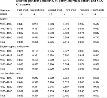
Table 3: Proportion of women who have not given birth again 1.5 and 4 years after the previous childbirth, by parity, marriage cohort, and SES. Granarolo
Marriage cohort
First child – Second child Second child – Third child Third child –Fourth child
1.5 4 1.5 4 1.5 4
All SES
1900‒1909 0.848 0.250 0.903 0.326 0.932 0.414 1910‒1919 0.858 0.331 0.925 0.435 0.931 0.563 1920‒1929 0.892 0.404 0.940 0.583 0.974 0.647 1930‒1940 0.922 0.540 0.969 0.684 0.999 0.740 Total 0.885 0.395 0.935 0.515 0.956 0.569
Sharecroppers and farmers
1900‒1909 0.824 0.194 0.875 0.327 0.899 0.337 1910‒1919 0.856 0.331 0.878 0.290 0.917 0.513 1920‒1929 0.866 0.405 0.930 0.575 0.957 0.650 1930‒1940 0.903 0.535 0.990 0.694 0.974 0.539 Total 0.866 0.384 0.920 0.483 0.935 0.526 Landless labourers
1900‒1909 0.851 0.247 0.939 0.262 0.946 0.536 1910‒1919 0.844 0.326 0.960 0.522 0.906 0.594 1920‒1929 0.904 0.341 0.945 0.507 0.985 0.616 1930‒1940 0.932 0.527 0.935 0.700 0.996 0.711 Total 0.888 0.354 0.945 0.480 0.966 0.597
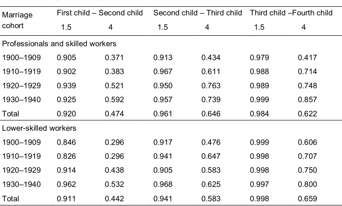
Table 3: (Continued)
Marriage cohort
First child – Second child Second child – Third child Third child –Fourth child
1.5 4 1.5 4 1.5 4
Professionals and skilled workers
1900‒1909 0.905 0.371 0.913 0.434 0.979 0.417 1910‒1919 0.902 0.383 0.967 0.611 0.988 0.714 1920‒1929 0.939 0.521 0.950 0.763 0.989 0.748 1930‒1940 0.925 0.592 0.957 0.739 0.999 0.857 Total 0.920 0.474 0.961 0.646 0.984 0.622 Lower-skilled workers
1900‒1909 0.846 0.296 0.917 0.476 0.999 0.606 1910‒1919 0.826 0.296 0.941 0.647 0.998 0.707 1920‒1929 0.914 0.438 0.905 0.583 0.998 0.750 1930‒1940 0.962 0.532 0.968 0.625 0.997 0.800
Total 0.911 0.442 0.941 0.583 0.998 0.659
Spacing and stopping might both play a role in the length of time between childbirths. Especially in the highest parities, the figures probably represent an increase in the proportion of those stopping their fertility career.
The increase in the postponement of the next birth is evidenced by the growth of the proportion of women who have not given birth again after the previous childbirth, which starts first in the higher-order births, following the classical scheme of fertility transition. Indeed, the biggest increases in the passage from the second to the third child and from the third to the fourth child begin with the 1920 marriage cohorts, while for the transition from the first to the second child the delay is more evident only in the 1930‒1940 marriage cohort.
Overall, the interval between births gets longer as the parity progresses. Differences between marriage cohorts are apparent for all of the transitions. Half of the women in the oldest marriage cohort (1900‒1909) had a second child 2.2 years after the
first birth, 20 whereas in the most recent marriage cohort about 75% of women had not
had a second child by this time. Around 50% of women wait more than 2.5 years to have a third child in the oldest marriage cohort, whereas this percentage rises to above 75% for the most recent marriage cohort.
Data by SES shows a general propensity to delay the time to second or higher-order childbirths for the nonagricultural social strata. This trend is particularly clear for the transition from the second to third child: More than 70% of professionals and skilled workers have not had a third child four years after the second childbirth, while the proportions are lower for agricultural workers. The relationship is less evident for the next parity progression, probably due to low numbers; however, the difference between the rural and nonrural SES groups is still evident.
The analysis of fertility by SES group raises various points of discussion. The indexes show that the fertility transition began with the marriage cohorts formed after
the beginning of the 20th century. The reductions in fertility from cohort to cohort
follow the two well-known paths, a decrease in high parities and an increase in the postponement of births. Some of these delays probably turn into stopping.
There is a general convergence of fertility behaviour downwards, but the decrease is not uniform for all SESs. Nor is the decreasing path uniform by SES: Sharecroppers remain at higher levels and with higher parities while having an earlier-marriage model.
6.2 Event history analysis of birth intervals
In this section we carry out a multivariate analysis to deepen our understanding of the results shown in the descriptive part of the paper.
We use event history methods to estimate the relative risks of having a second birth, a third birth, and other higher-parity births, while taking into account a number of factors that are known to have varied during the analysed period. As covariates, we consider the marriage cohort, the SES of the head of the family, the age of the woman, and the survival of the previous child (Table 4).
To evaluate socioeconomic differences in marital fertility during the fertility transition we estimate a Cox proportional hazards model, controlling for a basic set of
covariates (Therneau and Grambsch 2000).21 The duration variable is the time elapsed
from the previous birth, and we deal with closed intervals from one parity to the next. For the higher-order births we added a frailty term at the woman-level to account for correlation due to repeated events for the same mother (Box-Steffensmeier, De Boef, and Joyce 2006). The frailty term is assumed to follow a Gamma distribution (Therneau and Grambsh 2000).
The age of the woman and the life status of the previous child are time
dependent,22 while marriage cohort and SES are time invariant.
Table 4: Percentage distribution of covariates at marriage and first, second, and third child. Granarolo
Covariate Marriage First child Second child Third child
Age of woman
<25 70.76 64.44 31.98 13.50 25‒29 21.79 27.35 43.99 42.83 >29 7.44 8.21 24.03 43.67
Socioeconomic status
Sharecroppers and farmers 44.52 46.19 47.86 50.33 Landless labourers 28.31 27.86 28.10 29.33 Professionals and skilled workers 14.88 14.44 13.51 10.67 Lower-skilled workers 12.29 11.51 10.53 9.67
Marriage cohort
1900‒1909 17.41 17.60 21.85 29.83 1910‒1919 17.87 17.60 18.97 22.17 1920‒1929 38.87 38.93 38.73 33.67 1930‒1940 25.85 25.88 20.46 14.33
Child death
Alive 97.65 96.13 95.50
Death 2.35 3.87 4.50
N. of women 1,505 1,364 1,007 600
To control for the effect of infant mortality on fertility, a covariate of the life status of the previous child is included in the models. Several studies show that infant mortality can potentially affect natural fertility (Knodel 1988; Preston 1978). Indeed, a positive association between the two variables has been found in many pretransitional
populations, mainly due to biological reasons.23 At the end of the transition, when
couples have already achieved their target family size, a substitution effect still exists as
23 High infant mortality produces a shortening of birth intervals due to the mechanical action of the end of
the consequence of a rational choice. At the beginning of the transition when infant mortality is declining steadily the substitution effect could work differently: Couples could voluntarily react to an unexpected infant death before having achieved their target family size. For our marriage cohorts, infant mortality has already decreased and parents have experienced higher infant survival.
The age of the woman at the birth of her children operates as a control in the model, linked to the physiological and biological capacity of giving birth. We have created a categorical covariate consisting of three age groups, with under-25 as the
reference category. We expect a declining risk of childbirth as age increases.24
With regard to SES, and according to our research hypothesis, a higher probability of birth is expected for women living in sharecropping households, as sharecroppers needed larger household sizes and children represented an asset in their domestic economies. For them, the joint play of adjustment and innovation could result in slower decreasing fertility than for the other SES groups. The sharecropper contract functions as a social barrier, isolating sharecroppers in a more traditional framework of household economics and making this social group less permeable to both innovation and to shock events such as wars and other disasters.
Landless labourers, on the other hand, are expected to have lower fertility, since children did not play the same role in their household organization. The socioeconomic groups not involved in the agricultural sector are expected to be more susceptible to new attitudes concerning fertility, according to their social status. Thus, lower fertility levels are expected for professionals and skilled workers, while the less-skilled are expected to resemble more the landless labourers.
As the demographic transition moves forward, it is expected that behaviours will tend to slowly converge, with the social groups who started later speeding up the decrease in their fertility. The couples belonging to the different SESs begin to adjust their fertility targets, following their own paths according to the socioeconomic changes progressively taking place.
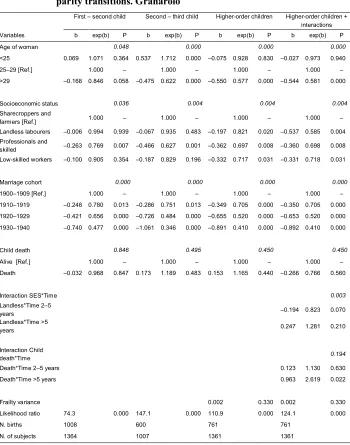
Table 5 shows relative risks deriving from Cox models for intervals between first and second birth, second and third birth, and for parities greater than three. In Tables 5 and 6 we also report the p-value for each variable, obtained by fitting the model with and without the variable under investigation and comparing the maximized log likelihoods.
24 We tested the age of the woman at the beginning of the birth interval as a time-constant variable (e.g., at
Table 5: Cox hazard estimates of having another child. Models for different parity transitions. Granarolo
First ‒ second child Second ‒ third child Higher-order children Higher-order children + interactions
Variables b exp(b) P b exp(b) P b exp(b) P b exp(b) P
Age of woman 0.048 0.000 0.000 0.000
<25 0.069 1.071 0.364 0.537 1.712 0.000 ‒0.075 0.928 0.830 ‒0.027 0.973 0.940
25‒29 [Ref.] 1.000 ‒ 1.000 ‒ 1.000 ‒ 1.000 ‒
>29 ‒0.168 0.846 0.058 ‒0.475 0.622 0.000 ‒0.550 0.577 0.000 ‒0.544 0.581 0.000
Socioeconomic status 0.036 0.004 0.004 0.004
Sharecroppers and
farmers [Ref.] 1.000 ‒ 1.000 ‒ 1.000 ‒ 1.000 ‒
Landless labourers ‒0.006 0.994 0.939 ‒0.067 0.935 0.483 ‒0.197 0.821 0.020 ‒0.537 0.585 0.004 Professionals and
skilled ‒0.263 0.769 0.007 ‒0.466 0.627 0.001 ‒0.362 0.697 0.008 ‒0.360 0.698 0.008
Low-skilled workers ‒0.100 0.905 0.354 ‒0.187 0.829 0.196 ‒0.332 0.717 0.031 ‒0.331 0.718 0.031
Marriage cohort 0.000 0.000 0.000 0.000
1900‒1909 [Ref.] 1.000 ‒ 1.000 ‒ 1.000 ‒ 1.000 ‒
1910‒1919 ‒0.248 0.780 0.013 ‒0.286 0.751 0.013 ‒0.349 0.705 0.000 ‒0.350 0.705 0.000
1920‒1929 ‒0.421 0.656 0.000 ‒0.726 0.484 0.000 ‒0.655 0.520 0.000 ‒0.653 0.520 0.000
1930‒1940 ‒0.740 0.477 0.000 ‒1.061 0.346 0.000 ‒0.891 0.410 0.000 ‒0.892 0.410 0.000
Child death 0.846 0.495 0.450 0.450
Alive [Ref.] 1.000 ‒ 1.000 ‒ 1.000 ‒ 1.000 ‒
Death ‒0.032 0.968 0.847 0.173 1.189 0.483 0.153 1.165 0.440 ‒0.266 0.766 0.560
Interaction SES*Time 0.003
Landless*Time 2–5
years ‒0.194 0.823 0.070
Landless*Time >5
years 0.247 1.281 0.210
Interaction Child
death*Time 0.194
Death*Time 2‒5 years 0.123 1.130 0.630
Death*Time >5 years 0.963 2.619 0.022
Frailty variance 0.002 0.330 0.002 0.330
Likelihood ratio 74.3 0.000 147.1 0.000 110.9 0.000 124.1 0.000
N. births 1008 600 761 761
We preliminary tested proportionality assumptions of the risks, using the Schoenfeld residuals test (Therneau and Grambsh 2000). In the case of the higher order births model only, the tests were statistically significant for the covariates ‘landless labourers’ and ‘death of the previous child’. To properly fit the Cox model we interacted these two variables with a step function defined over three different time
intervals (0‒2 years, 2‒5 years, more than 5 years)25 (Therneau, Crowson, and Atkinson
2017). Consequently, for the higher order parities we show two models, depending on whether only the principal effects or also the interaction with time are considered.
Two aspects are important, the demographic transition shown by the marriage cohorts and the declining fertility shown by the different SES groups, while the other covariates are boundary conditions. It is also necessary to remember that the outbreak of World War I inevitably had a strong influence on the stability of households and could confound the path towards innovation.
The effects of marriage cohort confirm the gradual development of the demographic transition: The coefficients reveal a statistically significant reduction in the risks of having another child for all of the transitions in all models. All of the cohorts show a progressive increase in birth intervals, and the hazard decreases more than 50% between the first cohort and the last. As stated in the descriptive section of this paper, this fact should be read as the joint effect of lengthening and stopping.
The role of SES shows interesting features. Until the birth of the third child, only the behaviour of professionals and skilled workers emerges statistically, across all transitions.
No statistically significant differences exist in the transition to second childbirth among rural SES groups (Table 5), while for higher-than-third-order children, sharecroppers and farmers maintain their primacy in high fertility level. The statistical significance of the parameters for higher-order children establishes a ranking between rural workers and the others, who show a more extreme downward trajectory in the hazard of having another child. These patterns are explained by the decrease in higher parities for all SES groups. This is particularly strong for nonagricultural households, underlining the increasing length of intervals between births, and perhaps more frequent stopping behaviour among nonrural families. Our results confirm previous studies which observe that sharecropper women show higher fertility levels than rural (landless) daily labourers in the pretransitional period (Breschi et al. 2014).
Throughout the first decades of the 20th century the results reveal a stronger link to
traditional reproductive behaviour for agricultural SES, especially for sharecroppers and farmers, while nonagricultural workers in high social classes continue to show lower
fertility. It is useful to remember that in the first marriage cohort the difference between the TMFRs of these SES groups is wide, varying between 5.91 and 4.81. Thus, at the beginning of the observed period the different social classes started at different levels of fertility transition, and at the end of the observation the total marriage fertility rate is 1.1 children lower for sharecroppers and farmers and 0.5 lower for professionals and skilled workers. It is therefore interesting to note that the downward trend in fertility seems to cross all social groups, although there are distinct differences in the quantum of fertility. Indeed, in the more recent marriage cohort, sharecroppers show a higher fertility intensity than the other groups.
No statistical significance is detected for the time-dependent variable ‘death of previous child’ for the first and second parity transitions.
Table 5 compares the results of the two last models and includes the interaction with time. It shows that the risk of having another birth after the last child death
significantly increases for time intervals greater than 5 years.26 Following Knodel’s
theory (1988), the ‘replacement of descendants’ mechanism could result from a reaction to an unexpected infant death in the last phases of couples’ reproductive life.
In Table 5 the last model also includes an interaction term between the ‘landless labourers’ category and the time intervals. The coefficients are statistically significant
for the baseline 0‒2 years and the 2‒5-years interval.27 This result confirms the
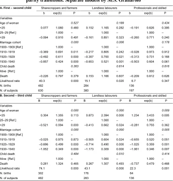
non-proportional decline over time for landless labourers with respect to the other groups. To further examine the relationship between fertility transition, cohort, and SES behaviour, we finally estimated the risk of having another child for each SES category separately. The hazards of the final models are shown in Table 6. We have excluded the SES group of lower-skilled workers because it has a lower number of events and observations than the others.
To solve non-proportional hazard assumptions, proved only for sharecroppers in the higher order parity transitions, we introduced an interaction term with time.
First, the results show the effects of the marriage cohorts on the different SES classes.
26 The net effect is equal to 2.007 [exp(-0.266+0.963)], a twice-higher hazard than the baseline.
Table 6: Cox hazard estimates of having another child. Models for different parity transitions. Separate models by SES. Granarolo
A. First – second child Sharecroppers and farmers Landless labourers Professionals and skilled
b exp(b) P b exp(b) P b exp(b) P
Variables
Age of woman 0.527 0.189 0.434
<25 0.077 1.080 0.480 0.152 1.165 0.282 ‒0.191 0.826 0.395
25‒29 [Ref.] 1.000 ‒ 1.000 ‒ 1.000 ‒
>29 ‒0.094 0.910 0.491 ‒0.161 0.851 0.323 ‒0.260 0.771 0.240
Marriage cohort 0.000 0.006 0.178
1900‒1909 [Ref.] 1.000 ‒ 1.000 ‒ 1.000 ‒
1910‒1919 ‒0.369 0.691 0.011 ‒0.217 0.805 0.242 ‒0.028 0.973 0.912
1920‒1929 ‒0.492 0.611 0.000 ‒0.357 0.700 0.021 ‒0.313 0.731 0.168
1930‒1940 ‒0.857 0.424 0.000 ‒0.653 0.521 0.001 ‒0.503 0.604 0.061
Child death 0.363 0.614 0.616
Alive [Ref.] 1.000 ‒ 1.000 ‒ 1.000 ‒
Death ‒0.226 0.797 0.379 0.153 1.166 0.607 ‒0.209 0.812 0.626
Likelihood ratio 40.3 0.000 15.1 0.020 6.7 0.347
N. births 482 284 136
N. of subjects 630 380 197
B. Second – third child Sharecroppers and farmers Landless labourers Professionals and skilled
B exp(b) P B exp(b) P B exp(b) P
Variables
Age of woman 0.000 0.000 0.009
<25 0.304 1.355 0.113 0.873 2.394 0.000 1.234 3.433 0.005
25‒29 [Ref.] 1.000 ‒ 1.000 ‒ 1.000 ‒
>29 ‒0.521 0.594 0.000 ‒0.413 0.662 0.024 ‒0.281 0.755 0.362
Marriage cohort 0.000 0.000 0.005
1900‒1909 [Ref.] 1.000 ‒ 1.000 ‒ 1.000 ‒
1910‒1919 ‒0.025 0.975 0.873 ‒0.505 0.604 0.024 ‒0.655 0.520 0.051
1920‒1929 ‒0.696 0.499 0.000 ‒0.714 0.490 0.000 ‒1.025 0.359 0.001
1930‒1940 ‒1.052 0.349 0.000 ‒1.173 0.309 0.000 ‒1.061 0.346 0.007
Child death 0.484 0.510 0.414
Alive [Ref.] 1.000 ‒ 1.000 ‒ 1.000 ‒
Death 0.281 1.324 0.465 0.267 1.307 0.493 ‒0.737 0.479 0.468
Likelihood ratio 74.1 0.000 43.1 0.000 22.3 0.001
N. births 302 176 64
Table 6: (Continued)
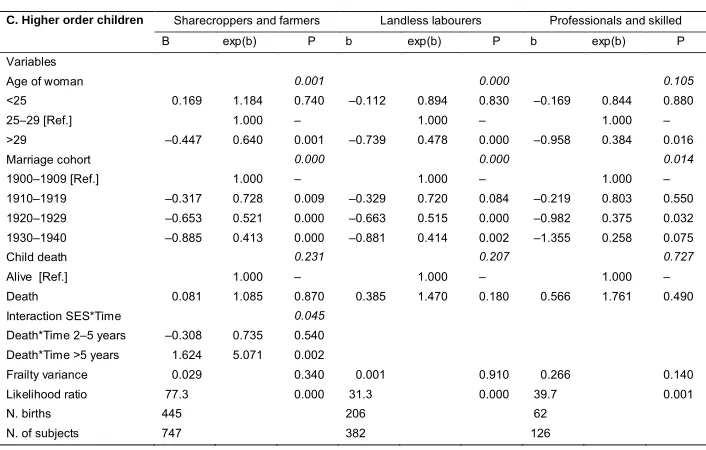
C. Higher order children Sharecroppers and farmers Landless labourers Professionals and skilled
B exp(b) P b exp(b) P b exp(b) P
Variables
Age of woman 0.001 0.000 0.105
<25 0.169 1.184 0.740 ‒0.112 0.894 0.830 ‒0.169 0.844 0.880
25‒29 [Ref.] 1.000 ‒ 1.000 ‒ 1.000 ‒
>29 ‒0.447 0.640 0.001 ‒0.739 0.478 0.000 ‒0.958 0.384 0.016
Marriage cohort 0.000 0.000 0.014
1900‒1909 [Ref.] 1.000 ‒ 1.000 ‒ 1.000 ‒
1910‒1919 ‒0.317 0.728 0.009 ‒0.329 0.720 0.084 ‒0.219 0.803 0.550
1920‒1929 ‒0.653 0.521 0.000 ‒0.663 0.515 0.000 ‒0.982 0.375 0.032
1930‒1940 ‒0.885 0.413 0.000 ‒0.881 0.414 0.002 ‒1.355 0.258 0.075
Child death 0.231 0.207 0.727
Alive [Ref.] 1.000 ‒ 1.000 ‒ 1.000 ‒
Death 0.081 1.085 0.870 0.385 1.470 0.180 0.566 1.761 0.490
Interaction SES*Time 0.045
Death*Time 2‒5 years ‒0.308 0.735 0.540
Death*Time >5 years 1.624 5.071 0.002
Frailty variance 0.029 0.340 0.001 0.910 0.266 0.140
Likelihood ratio 77.3 0.000 31.3 0.000 39.7 0.001
N. births 445 206 62
N. of subjects 747 382 126
When the age of the woman is controlled for, the risks of having a second child (Table 6a) decrease significantly for all marriage cohorts of sharecroppers and farmers, for the last two cohorts of landless labourers, and for the most recent cohort of professionals and skilled workers, revealing a lengthening of birth intervals in each situation. When we also observe the second–third transition (Table 6b) the results are opposite: The hazards decrease in all marriage cohorts of professionals and skilled workers and landless labourers, but only in the two most recent cohorts of sharecroppers and farmers. Finally, considering the transition from the third to highest parity (Table 6c), both agricultural SES groups still show a decreasing risk by marriage cohort, while the effect is significantly weaker for the nonrural social class.
These different effects suggest that the downward trends in fertility by parity and SES are unequal. The lengthening of the interval between first and second childbirth is likely to represent a spacing action, while for the transition to higher births, stopping behaviour probably has a stronger effect.
The decrease in fertility of the professionals and skilled workers is even stronger than for the other SES groups, although without being fully statistically significant.
The interaction of the variable ‘death of the previous child’ with time shows significant values for sharecroppers and farmers when longer than 5 years is considered. Considering this, and going back to the ‘substitution of the last child’ effect previously discussed in connection with Table 5, the significant interaction detected in that table can be mainly attributed to the group of sharecroppers and farmers.
We can summarize the most relevant aspects by combining the model findings with the descriptive statistics. Starting from the 1920‒1929 marriage cohort and for the professionals and skilled workers group, the downward trend in terms of hazards almost certainly is the result of stopping behaviour.
At the beginning of the observation period, professionals and skilled workers have the lowest TMFR20 and sharecroppers and farmers the highest. Sharecroppers and farmers in general start the fertility decline at higher levels but their behaviour tends to converge over time with that of the other social groups. Convergence is not yet reached with the last observed marriage cohort.
The 1920‒1929 cohort dates the beginning of consistent downwards fertility. World War I probably had a destabilizing effect on the path of the fertility transition.
By the last marriage cohort of rural workers the risk of having a higher parity child has almost halved, with even greater reductions for the lowest fertility group of professionals and skilled workers.
On the other hand, sharecroppers and farmers show persistently high fertility and a clear decline in the risk of higher order children after the first post-war marriage cohort, underlying a possible time lag in the fertility transition with respect to the other SES groups.
7. Final remarks
Granarolo is an apposite place to examine the path and structure of the fertility
transition in the first decades of the 20th century. This northern Italian village
maintained its rural character until the middle of the 20th century. In an area inhabited
by various SES groups, we have identified the specific subsystems of a still-rural society.
Using micro-level analysis we studied the fertility decline of the SES groups that lived in the area, in an effort to depict the different behaviours that lie behind the more general process of the demographic and fertility transition.
couples to make rational choices. This new behaviour is then mediated by the readiness of the couple and the household to adopt the new scheme if it is advantageous to the prosperity of the family group (Coale 1973). This readiness is linked to the social and economic background of each social group and to the economic evolution of the context in which it exists.
The results of our analysis can be summarised in some main points.
First, there is a clear drop in fertility from one marriage cohort to the next, which appears to be mainly linked to a decline in higher birth orders. The probability of giving birth progressively falls with each marriage cohort once women reach a high number of children.
The fertility transition proceeds by means of two known techniques, spacing and stopping. The descriptive analysis confirms the downward trend in high parities and shows the decline in age at last childbirth, which falls below 32 years for almost all SES groups. Sharecroppers and farmers show an age slightly higher than 32 years at the birth of the last child.
The propensity to concentrate childbirths at younger ages progressively increases with each new marriage cohort, as shown by the proportion of childbirths before 25 years of age. This is probably the result of women shortening the reproductive interval once they are able to control their fertility, thus reducing higher-order births.
Second, socioeconomic differentials matter. Among the SES categories the social groups ‘sharecroppers and farmers’ and ‘professionals and skilled workers’ stand out in terms of demographic behaviour. The first maintains the highest fertility, the second the lowest. However, there are clear differences between ‘landless labourers’ and ‘sharecroppers and farmers’.
Beyond these differences the data shows a general convergence of behaviours for all social classes, but socioeconomic factors before and during the transition are clearly at play in shaping the different timing and paths in the downward trend of fertility.
Sharecroppers and farmers are characterized by having the highest level of fertility. They exhibit higher fertility in the earliest marriage cohorts, but starting from the 1920‒1929 cohort they experience a decreasing path towards lower levels. However, they continue to have the highest levels and the highest parities, while having an earlier-marriage model.
The landless labourers show a stronger reduction in higher parities and are more susceptible to shock events and changes in the socioeconomic context.
Finally, in a society which is still linked to agricultural and traditional values regardless of the proximity of the city, professionals and skilled workers are the most innovative in terms of number of offspring.
classes to the lower classes. However, this process does not hold in this rural world where the path is reversed from the lower to the upper groups, considering the sharecroppers and farmers as an upper rural social class, compared with landless labourers. For the sharecroppers and farmers the effect of belonging to a relatively well-off class is cancelled out by their unwillingness to reduce their well-offspring (Coale 1973).
Another striking element is that these trends do not lead to a marked widening of the socioeconomic differential during the transition. On the contrary, despite the fact that we cannot affirm that the decreasing trends are totally uniform in level, the convergence seems to happen in an almost homogeneous way. The moment at which all social groups begin to join the movement corresponds to the biographies of the 1930‒ 1939 new couples.
Finally, and going back to the historical period in which the fertility transition was
developing, data shows that in Granarolo fertility decline was an irreversible process28
that did not stop even when the fascist regime promoted a pro-birth campaign (Ipsen 1997).
References
Bardet, J.-P. (1983).Rouen aux XVIIe et XVIIIe siècles: Les mutations d’un espace
social(Vol. 1). Paris: Sedes.
Becker, G.S. (1981).A treatise on the family. Cambridge: Harvard University Press.
Bellettini, A. (1971). La popolazione delle campagne bolognesi alla metà del secolo
XIX. Bologna: Zanichelli.
Bengtsson, T. and Ohlsson, R. (1994). The demographic transition revisited. In:
Bengtsson, T. (ed.).Population, economy, and welfare. Berlin: Springer: 13‒36.
doi:10.1007/978-3-642-85170-4_2.
Bengtsson, T. and Dribe, M. (2014). The historical fertility transition at the micro level:
Southern Sweden 1815‒1939. Demographic Research 30(17): 493‒534.
doi:10.4054/DemRes.2014.30.17.
Bernardi, L. (2003). Channels of social influence on reproduction.Population Research
and Policy Review 22(5‒6): 427‒555.doi:10.1023/B:POPU.0000020892.15221. 44.
Bongaarts, J. (1978). A framework for analyzing the proximate determinants of fertility. Population and Development Review 4(1): 105‒132.doi:10.2307/1972149. Bongaarts, J. and Watkins, S.C. (1996). Social interactions and contemporary fertility
transitions. Population and Development Review 22(4): 639‒682. doi:10.2307/
2137804.
Box-Steffensmeier, J.M., De Boef, S., and Joyce, K.A. (2006). Event dependence and
heterogeneity in duration models: The conditional frailty model. Political
Analysis 15(3): 237‒256.doi:10.1093/pan/mpm013.
Bras, H. (2014). Structural and diffusion effects in Dutch fertility transition, 1870‒
1940. Demographic Research 30(5): 151‒186.doi:10.4054/DemRes.2014.30.5.
Breschi, M., Esposito, M., Mazzoni, S., and Pozzi, L. (2014). Fertility transition and
social stratification in the town of Alghero, Sardinia (1866‒1935).Demographic
Research 30(28): 823‒852.doi:10.4054/DemRes.2014.30.28.
Breschi, M., Fornasin, A., Pozzi, L., Rettaroli, R., and Scalone, F. (2009). The onset of fertility transition in Italy 1800‒1900. In: Fornasin, A. and Manfredini, M.
(eds.).Fertility in Italy at the turn of the 20th century. Udine: Forum: 11‒29.
Breschi, M., Manfredini, M., and Rettaroli, R. (2000). Comportamento riproduttivo e contesto familiare in ambito rurale: ‘Case-studies’ sull’Italia di pre-transizione. Popolazione e storia 1(1‒2): 199‒216.
Breschi, M., Pozzi, L., and Rettaroli, R. (1994). Analogie e differenze nella crescita
della popolazione italiana, 1750,1911. Bollettino di Demografia Storica 20:
41,94.
Caldwell, J.C. (1982).Theory of fertility decline. London: Academic Press.
Carlsson, G. (1966). The decline of fertility: Innovation or adjustment process. Population Studies 20(2): 149‒174.doi:10.1080/00324728.1966.10406092. Carter, A.T. (2001). Social processes and fertility change: Anthropological
perspectives. In: Casterline, J.B. (ed.). Diffusion processes and fertility
transition: selected perspectives. Washington, D.C.: National Academy Press: 138–178.
Casterline, J.B. (2001). Diffusion processes and fertility transition: Introduction. In:
Casterline, J.B. (ed.). Diffusion processes and fertility transition: Selected
perspectives. Washington, D.C.: National Academy Press: 1‒38.
Cazzola, F. (1996). Storia delle campagne padane dall’Ottocento a oggi. Milano:
Mondadori.
Cleland, J. (2001). Potatoes and pills: An overview of innovation-diffusion contributions to explanations of fertility decline. In: Casterline, J.B. (ed.). Diffusion processes and fertility transition: Selected perspectives. Washington,
D.C.: National Academy Press: 39,65.
Cleland, J. and Wilson C. (1987). Demand theories of the fertility transition: An
iconoclastic view. Population Studies 41(1): 5‒30. doi:10.1080/00324720310
00142516.
Coale, A.J. (1967). The voluntary control of human fertility.Proceedings of the
American Philosophical Society 111(3): 164‒169.
Coale, A.J. (1969). The decline of fertility in Europe from the French Revolution to
World War II. In: Behrman, S.J., Corsa, Jr., L., and Freedman, R. (eds.). Fertility