R E S E A R C H A R T I C L E
Open Access
What has driven the evolution of multiple cone
classes in visual systems: object contrast
enhancement or light flicker elimination?
Shai Sabbah
1*and Craig W Hawryshyn
1,2Abstract
Background:Two competing theories have been advanced to explain the evolution of multiple cone classes in vertebrate eyes. These two theories have important, but different, implications for our understanding of the design and tuning of vertebrate visual systems. The‘contrast theory’proposes that multiple cone classes evolved in shallow-water fish to maximize the visual contrast of objects against diverse backgrounds. The competing‘flicker theory’states that multiple cone classes evolved to eliminate the light flicker inherent in shallow-water
environments through antagonistic neural interactions, thereby enhancing object detection. However, the selective pressures that have driven the evolution of multiple cone classes remain largely obscure.
Results:We show that two critical assumptions of the flicker theory are violated. We found that the amplitude and temporal frequency of flicker vary over the visible spectrum, precluding its cancellation by simple antagonistic interactions between the output signals of cones. Moreover, we found that the temporal frequency of flicker matches the frequency where sensitivity is maximal in a wide range of fish taxa, suggesting that the flicker may actually enhance the detection of objects. Finally, using modeling of the chromatic contrast between fish pattern and background under flickering illumination, we found that the spectral sensitivity of cones in a cichlid focal species is optimally tuned to maximize the visual contrast between fish pattern and background, instead of to produce a flicker-free visual signal. Conclusions:The violation of its two critical assumptions substantially undermines support for the flicker theory as originally formulated. While this alone does not support the contrast theory, comparison of the contrast and flicker theories revealed that the visual system of our focal species was tuned as predicted by the contrast theory rather than by the flicker theory (or by some combination of the two). Thus, these findings challenge key assumptions of the flicker theory, leaving the contrast theory as the most parsimonious and tenable account of the evolution of multiple cone classes.
Keywords:Contrast hypothesis, Cone photoreceptors, Critical fusion frequency, Temporal contrast sensitivity, Opponent mechanisms, Color vision, Retina, Fish
Background
Multiple spectral classes of cones are found in the visual system of many vertebrates [1]. Comparison of the outputs of different cone classes enables color vision. Multiple cone classes appeared very early in vertebrate evolution, at least 540 MYA (million years ago) and perhaps as early as 700 MYA, prior to the separation of the jawed (Gnathostomata) and jawless (Agnatha) vertebrate lineages (approximately 485 MYA) [2,3]. This is based on the
presence of five classes of cone-like photoreceptors in the
jawless Southern Hemisphere lamprey, Geotria australis
[4-6], and three cone classes in the jawed cartilaginous fishes (Chondrichthyes) [7-9]. Additionally, cone opsins have been suggested to evolve prior to rod opsins [10], indicating that photopic (bright light) vision preceded scotopic (dim light) vision, and suggesting that these early vertebrates occupied brightly-lit shallow-water environ-ments [11]. However, although the evolution of visual pigments has been studied extensively [1,4,6,10,12-20], the selective pressures that have driven the evolution of multiple cone classes in the eyes of vertebrates remain largely obscure.
* Correspondence:[email protected] 1
Department of Biology, Queen’s University, Kingston, Ontario K7L 3N6, Canada
Full list of author information is available at the end of the article
Two competing theories have been advanced to explain the evolution of multiple cone classes; both assumed that vision in ancestral vertebrates utilized multiple cone photoreceptor classes, with color vision evolving only later
as a byproduct. The ‘contrast theory’ of Munz and
McFarland and McFarland and Munz [13,14] proposed that multiple cone classes evolved in shallow-water fish to maximize the visual contrast between objects and their background. Indeed, a single visual pigment (either rod or cone) may suffice to maximize the visual contrast between a given object and background. However, the need to maximize contrast between diverse objects and back-grounds of varying brightness and spectral characteristics was suggested to favor the appearance of multiple cone
classes. The competing ‘flicker theory’ presented by
Maximov [21] proposed that multiple cone classes have evolved to allow elimination of the flicker (fluctuation in light intensity) produced by variation in the refraction of sunlight at the water surface [22-25]. It was argued that subtraction of the output of one cone class from another through antagonistic (opponent) neural interac-tions would filter out the light flicker, yielding a flicker-free representation of the visual scene and enhancing object detection. The flicker theory has received relatively little attention; however, it has remained a competitor of the contrast theory, leaving the forces that have driven the evolution of multiple cone classes an open question.
Both the contrast and flicker theories assume the presence of at least two cone classes that differ in spectral tuning. The flicker theory rests on three additional as-sumptions, one of which is the presence of antagonistic interactions between the output signals of the available cone classes. This assumption receives support from the presence of color-opponent horizontal cells [26,27] and the concentrically-antagonistic center-surround organization in retinal bipolar [28,29] and ganglion cells [30] in lower vertebrates. At least some of these color opponent mecha-nisms were probably present in early vertebrates that are represented today by the jawless lampreys [31-33]. However, two other critical assumptions of the flicker theory have so far not been seriously examined. First, it is assumed that ‘the [light] fluctuations are colorless, that is, the intensity of light changes synchronously in different parts of the spectrum’[21]. Consequently, despite the strong fluctuations in light over the entire spectrum, the ratio of light intensities in two different parts of a spectrum would remain constant, and would depend only on the spectral properties of the viewed object. Second, the flicker theory assumes that ‘the significant flicker of illumination inherent in the shallow-water environment complicated the visual process in the achromatic case, in particular preventing early detection of enemies’ [21]. Thus, because light flicker would impair object detection, selection would favor removal of light flicker from the
processed visual signal. These critical assumptions of the flicker theory have never been tested.
In this report, we evaluated the relative merits of the contrast and flicker theories. We first focused on the two largely untested assumptions of the flicker theory, and then asked whether the predictions of the two theories regarding the spectral tuning of cone pigments are supported by the evidence. We found that the amplitude and temporal frequency of light flicker are wavelength dependent and that the flicker may actually enhance the detection of objects, thus violating critical assumptions of the flicker theory. While this alone does not support the contrast theory, comparison of the contrast and flicker theories by means of chromatic contrast modeling under flickering illumination revealed that the spectral tuning of cone pigments of a focal cichlid species produced a large chromatic contrast between background and the body pattern of fish, and did not allow elimination of temporal fluctuations in the visual signal. This suggests that the visual system of the focal species is tuned as predicted by the contrast theory rather than by the flicker theory (or by some combination of the two).
Results and discussion
Amplitude and temporal frequency of flicker are wavelength dependent
The first critical assumption of the flicker theory is that
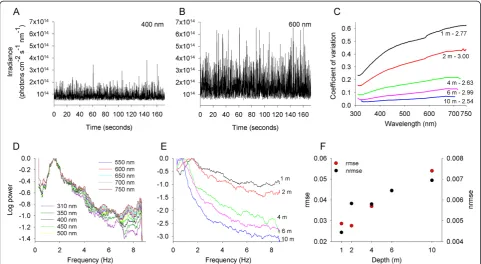
frequency of flicker decreased with increasing depth (Figure 1E). The wavelength dependence of the power distribution of flicker also varied with water depth, such that the wavelength dependence of the power distribution became weaker with increasing depth (Figure 1F). These findings are consistent with variation observed in the wavelength dependence of the power distribution of light flicker across different viewing orientations [34]. (See Additional file 2 for similar analysis for sideward irradiance.) Light flicker is produced by the focusing and defocusing of sunlight rays refracted at the water surface [22,24]. The wavelength dependence of the ampli-tude and temporal frequency of the flicker arises largely from variation in the scattering of light across the spectrum. Scattering at short wavelengths by molecules and small particles in the atmosphere and water is generally more pronounced than at long wavelengths. This causes short-wavelength light to be more diffused and conse-quently less affected by the wave-focusing phenomenon
than long-wavelength light. Therefore, our results demonstrate that the amplitude of the flicker and the distribution of its power across temporal frequencies vary across the light spectrum, violating the flicker theory’s first assumption.
Subtraction of cone outputs through opponent channels does not produce a flicker-free visual signal
We examined the effect of the wavelength depend-ence of light flicker on the output of cones and on the capacity of a simple subtraction of cone outputs to eliminate the flicker from the processed signal. To this end, we calculated the cone output (estimated by the quantum catch of cone pigments) when viewing an achromatic target (reflectance = 50% across the spectrum) under flickering illumination in a focal
spe-cies, Metriaclima zebra (a Lake Malawi cichlid). The
cone pigment complement found in adult M. zebra
includes the SWS1 (368 nm), Rh2b (484 nm), and
Figure 1Amplitude and temporal frequency of the light flicker of downward irradiance are wavelength dependent. (A,B)Examples of light flicker time series of downward irradiance at 1 m depth and light wavelengths of 400 and 600 nm. Each time series constitutes of 3,000 measurements acquired over 173 s. The amplitude of the light flicker at 600 nm is larger than at 400 nm.(C)The amplitude (estimated as the coefficient of variation) of light flicker of downward irradiance decreased with growing water depth (across the 1 to 10 m depth range), and increased monotonically toward longer light wavelengths. The ratio between the amplitude at the longest and shortest wavelengths was calculated for each depth. This ratio did not vary considerably across depths, and ranged between 2.5 and 3.0 (presented next to each spectrum).
Rh2a (523 nm) pigments (wavelength values represent
the wavelength of maximum absorbance of cones, λmax)
[36]. The target viewed was assumed to be illuminated by flickering sideward irradiance at a depth of 1 m, and cones were assumed to be adapted to the mean sideward irradi-ance at the same depth. (See the Methods section for de-tailed description of how cone and opponent channel outputs were calculated).
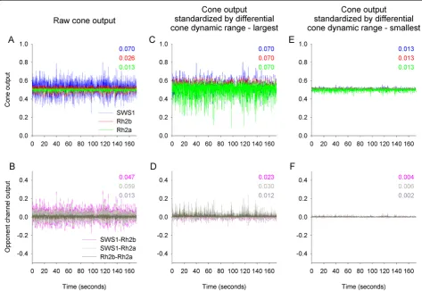
Cone output varied considerably over time under flickering illumination, with the variation in cone output (estimated as the standard deviation over time) decreasing when moving from SWS1 (0.070), through Rh2b (0.026), and to Rh2a (0.013) (cone output is unitless because it is normalized by the adapting light) (Figure 2A). The output among the three cones varied because long wavelength pigments such as Rh2b and Rh2a show broad sensitivity
functions, with both the α- and β-absorption bands in-cluded in the 300 to 800 nm spectrum that might be used for vision. By sampling the light flicker across the spectrum, the broad sensitivity functions act to reduce the variation of cone output produced under wavelength-dependent flickering illumination. In contrast, short wave-length pigments such as SWS1 show narrow sensitivity functions, with only the α-absorption band included in the 300 to 800 nm spectrum. These narrow sensitivity functions act to increase the variation in cone output.
The configuration of color opponent channels in M.
zebra is currently unknown. Thus, we modeled three possible opponent channels, that is, Rh2b, SWS1-Rh2a, and Rh2b-Rh2a. Output of opponent channels subjected to flickering illumination varied over time, showing variation largely comparable to that in the
output of cones (SWS1-Rh2b, 0.047; SWS1-Rh2a, 0.059; and Rh2b-Rh2a, 0.013) (Figure 2B). Therefore, contrary to the prediction of the flicker theory, simple subtraction of the output of one cone class from that of another through opponent interactions would not produce flicker-free output signal.
Certain modifications to the flicker theory would potentially allow the intended generation of flicker-free visual signals. An obvious way to generate a flicker-free visual signal would be to route the cone output through a low pass filter. This would attenuate any high frequency components in the signal, possibly producing flicker-free opponent channel signals. Such filtration, however, would inevitably reduce the temporal resolution by which the animal is sampling the environment, compromising the animal’s ability to detecting fast moving and changing stimuli, and reacting to them. Furthermore, considering the wavelength dependence of the power distribution of flicker (discussed above), even the low frequency components that are allowed to pass the filter would differ slightly between different cone classes; that is, even opponent channels that only use the low frequency com-ponents would not produce a flicker-free signal. Therefore, the use of low pass filtration for generating flicker-free visual signals comes with high cost, and is unlikely to provide a selective advantage.
Adjusting the dynamic range of cones would also potentially allow generation of flicker-free opponent channel output. For example, if the dynamic range of cones were to vary such that variation in cone output across the three cone classes was equalized over time, then subtraction of cone output through opponent channels would potentially produce a flicker-free signal. To test this possibility, we artificially adjusted the dynamic range of cones so that the variation over time in cone output was similar for all cone classes and equaled that of the SWS1 cone that exhibited the largest variation (Figure 2C). Following the dynamic range adjustment, the variation in opponent channels’output decreased only slightly, and did not produce flicker-free visual signals (SWS1-Rh2b, 0.023; SWS1-Rh2a, 0.030; and Rh2b-Rh2a, 0.012) (Figure 2D). Additionally, such differential adjustment of the dynamic range of cones would reduce the resolution in which the incident color signals (radiance) that vary in intensity are being sampled, potentially compromising the discrimination between targets of relatively close spectral reflectance characteris-tics. We also artificially adjusted the dynamic range of cones such that the variation in cone output over time was similar for all cone classes, but now, equaled to that of the Rh2a cone that exhibited the smallest variation (Figure 2E). Following this second dynamic range
ad-justment, the variation in opponent channels’ output
decreased by an order of magnitude, producing a visual
signal that is almost flicker-free (SWS1-Rh2b, 0.004; SWS1-Rh2a, 0.006; and Rh2b-Rh2a, 0.002) (Figure 2F). Thus, such a mechanism may theoretically generate a flicker-free output of opponent channels. Note however, that such differential adjustment of the dynamic range of cones to span the dynamic range of the cone that shows the narrowest dynamic range would result in failure to sample many incident color signals that fall outside of this narrow dynamic range. This would substantially com-promise the detection of targets of various spectral reflect-ance characteristics, which are illuminated by a range of irradiance levels. Therefore, this possibility is also highly unlikely to have a selective advantage.
Nevertheless, the implementation of complex antag-onistic interactions between cone classes (for example, SWS1 + Rh2b - Rh2a), may potentially allow the intended generation of flicker-free visual signals. However, as our light flicker measurements show, the dominant fre-quency, the frequency distribution of flicker, and the wavelength dependence of the power distribution of flicker all vary with water depth. This suggests that a fixed,‘wired’compensation for the wavelength depend-ence of flicker would fail when an animal moves in the water column or views objects at different lines of sight; behaviors that are common to many fish. In sum-mary, contrary to the prediction of the flicker theory, sim-ple subtraction of the output of one cone class from that of another through opponent interactions would not pro-duce a flicker-free output signal. Moreover, neither fixed low pass filtration nor adjustment of the dynamic range of cones would likely to be favored. Thus, although there might be a mechanism by which flicker-free visual signals would be generated under flickering illumination, the like-lihood of such a possibility is low, and the likelike-lihood that such a possibility would be favored either by natural or sexual selection is even lower.
Temporal frequency of light flicker matches the frequency where maximum contrast sensitivity in fish is attained
A second assumption of the flicker theory is that flicker interferes with object detection. However, by generating periodic changes in the retinal image, flicker may enhance perception [37] and detection of coarse (low spatial frequency) patterns [38]. The flicker is analogous to the flashing of an artificial light, such as a turn signal on a car; it is visually prominent because of the extreme brightness change, and possibly because of an unknown visual alertness system. This enhancement of object appearance would be most efficient if the temporal frequency of the flicker matched the frequency where maximum contrast sensitivity (Fmax) is attained [35,39,40].
species, the goldfish (Carassius auratus) [41], while the temporal contrast sensitivity of fish has often been studied through the measurement of the critical fusion frequency (CFF), the frequency at which temporally modulated light stimuli appear to fuse and have constant brightness. The temporal contrast sensitivity function varies with the adaptation state of the eye, the mean intensity of the modulated light stimulus, the visual angle subtended by the stimulus beam, and the temperature. Nevertheless, it still takes on a rather simple and easily modeled function [42-44], where Fmaxtypically ranges between 10% and 20%
of CFF [41,45-48]. Thus, to accommodate comparison between the frequency of wave-induced light flicker and the Fmaxof various fish species, as a first-order approximation,
Fmaxwas estimated as 15% of CFF, and then as either 10%
or 20% of CFF, covering the possible realistic range of relationships between Fmaxand CFF.
We compiled CFF data for 47 fish species, representing 41 genera, 34 families, and 14 orders, including both bony and cartilaginous fishes. See Additional file 3 for compil-ation of CFF data and Fmaxestimates with reference to the
light adaptation regime and temperature used during experiments, as well as the habitat and depth distribution of each species. Fmaxvaried with stimulus intensity, light
adaptation regime, and temperature. Nonetheless, with Fmax estimated as 15% of CFF, the distribution of Fmax
values across frequency corresponded well to the power spectrum of the light flicker, being highest at the domin-ant frequency of the flicker (Figure 3A). To support our findings further, we calculated the cumulative power of the flicker across temporal frequencies, which, unlike the dominant frequency of the flicker, is rather robust to
variation in surface wave conditions. The median Fmax
for dim stimuli, 1.8 Hz, matched the frequency below which close to 50% of the cumulative power of flicker
was found at 1 m depth. The median Fmax for bright
stimuli, 3.5 Hz, matched the frequency below which between 50% and 90% of the cumulative power of flicker was found at 1 m depth (Figure 3B). The relative power at high frequencies decreased with increasing depth.
Yet, the median Fmax for both dim and bright stimuli
matched the frequency below which 99% of the cumula-tive power was found at 10 m depth, for which the relacumula-tive power at high frequencies was the lowest (Figure 3B; Additional file 1E-G). A similar trend was observed
when Fmaxwas estimated as either 10% or 20% of CFF
(Additional file 4). Therefore, these findings suggest that light flicker may enhance the detection by fish of under-water objects under a range of light intensities and under-water depths, violating the flicker theory’s second assumption.
Note that the correspondence between the Fmaxof fish
and the frequency of flicker might potentially break if the fish species included in the analysis were to change.
This is especially important if Fmax varied across
environmental categories such as habitat type and depth. Species were classified based on their habitat type as being either ‘benthic’,‘benthopelagic’, or ‘pelagic’species. Species were also classified as inhabiting either ‘deep’ (typically found in depths >30 m), ‘shallow’ (typically found in depths <30 m), or both deep and shallow (‘shallow-deep’) habitats. As for the comparison be-tween Fmax and flicker frequency, the analysis included
all 35 fish species for which Fmaxdata were available for
both dim/natural and bright light stimuli (75% of cases) and were obtained under dark adaptation (80% of eligible pairs). The percentage of species inhabiting shallow (40%) and shallow-deep (46%) habitats was similar, whereas the percentage of strictly deep-water species was lower (14%). Moreover, the percentage of benthopelagic species (63%) was higher than those of either benthic (17%) or pelagic (20%) species (Figure 3C). Thus, if Fmaxdiffers between habitat or depth categories,
this may bias the comparison between Fmax and flicker
frequency. To test this possibility, we examined the effect of water depth and habitat type on the Fmaxof fish. Fmax
for bright stimuli differed significantly across habitat types
(randomization test (RT), df = 2, N = 35, P = 0.0098)
(Figure 3D). Post-hoc analysis revealed that Fmax in
benthic species was significantly lower than in either benthopelagic (P= 0.0095) or pelagic (P= 0.0012) species; Fmax in benthopelagic and pelagic species did not differ
significantly (P= 0.272). Moreover, Fmaxfor bright stimuli
did not differ significantly across depth categories (RT,
df = 2, N = 35, P = 0.4472) (Figure 3E). Fmax did not
differ significantly across depth categories also when fish from the‘shallow-deep’depth category were pooled with those from the‘shallow’category (RT, df = 1,N= 35, P= 0.6676) or with the‘deep’category (RT, df = 1,N= 35, P = 0.3231). Therefore, Fmax of fish does not vary with
habitat depth; however, Fmax of benthic species is lower
than in the other habitats. Consequently, if benthic species, that represent only 17% of the species analyzed, were to be represented better in the analysis, this would shift the distribution (and median) of Fmaxvalues toward
lower frequencies. Interestingly, inspection of Figure 3A,B reveals that this would actually improve the correspondence between Fmax of fish and the frequency of flicker, further
supporting our conclusions regarding a correspondence between the Fmaxof fish and flicker frequency.
Contrast theory versus flicker theory: a comparative analysis
multiple cone classes to increase the contrast of objects would have favored cone classes whose peak sensitivities are far apart. By contrast, using multiple cone classes to eliminate the light flicker would have favored cone classes whose peak sensitivities are the closest possible to each other. Nonetheless, providing conclusive evidence for the dominance of a given evolutionary pathway would require comparing the specific spectral locations of cone pigments of every fish species to the spectrum of ambient light under various conditions and for various behavioral contexts. Such a task is clearly impossible. Here instead, we chose to use a case study, a Lake Malawi cichlid, to as-sess whether the spectral location of cone pigments has
been shaped as predicted by the contrast theory or by the flicker theory, or by both.
For each opponent channel, we calculated responses to a range of naturally occurring body color patterns of fish (measured as diffused spectral reflectance) and the backgrounds against which the fish might be viewed under flickering illumination. The difference between these responses (ΔC) is a measure of the chromatic contrast of the particular opponent channel under these specific conditions. The model assigned spectral sensitivities to the cones based on the known characteristics of the cone
pigments in this fish. The cichlid Metriaclima zebra
belongs to the rock-dwelling Mbuna clade. In these
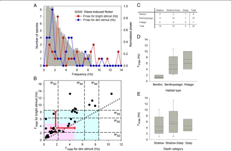
Figure 3Light flicker can enhance the detection of underwater objects. (A)Comparison between the frequency of light flicker in downward irradiance and the Fmaxof fish for dim and bright stimuli. The distribution of Fmaxvalues across frequency corresponded well to the
power spectrum of flicker across depths. Depicted power spectrum (gray shaded area) represents the envelope of flicker power across the 1 m and 10 m depth range.(B)Comparison between the cumulative power of the flicker and Fmaxfor dim and bright stimuli (closed circles). The
indices fP50, fP90, and fP99stand for the frequencies that correspond to 50, 90, and 99 percent of the cumulative power of flicker across
frequencies, averaged across the light spectrum. Vertical and horizontal dashed lines represent the fP50, fP90, and fP99values at 1 m depth. Gray
and pink shaded areas represent the frequency range enclosed by the 99% cumulative power bounds at 1 m and 10 m depth, respectively. (See Additional file 1E-G for the cumulative power indices as a function of light wavelength.) Fmaxdata points typically fell above the identity (dotted)
line, indicating larger Fmaxvalues for bright stimuli. The median Fmaxequaled 1.8 and 3.5 Hz, for dim and bright stimuli, respectively (open circle;
bidirectional red error bars represent the 25th and 75th percentiles).(C)Summary of the number of species inhabiting the various habitats and depths examined.(D,E)Association between the Fmaxof fish for bright stimuli and the habitat type (D) and water depth (E). Box specifications:
mean (dashed), median (solid), 25th and 75th percentiles; whiskers: 10th and 90th percentiles. For consistency, all analyses included only fish species for which Fmaxdata were available for both dim/natural and bright light stimuli (75% of cases), and were obtained under dark adaptation
species, males defend a territory in between rocks and perform elaborate displays to approaching females against the background of a vertical rock. Thus, following the contrast theory, the visual system would be designed to
ensure largeΔCmagnitude between the body patterns of
males and the background of rocks. However, following the flicker theory, the visual system would be structured to ensure smallΔCvariation under flickering illumination. The prediction regarding the contrast theory follows from the notion that the spectral location of visual pigments has evolved to maximize the chromatic contrast between the color pattern of males and their background. However, at least another possibility exists. That is, that the spectral location of visual pigments in females has been shaped by natural selection, and that males evolved body color patterns to maximize the chromatic contrast against their background, under those pre-existing visual system char-acteristics of females (‘sensory bias’hypothesis) [49]. The specific selection forces that have driven the spectral diversification of visual pigments in Lake Malawi cichlids are currently largely unknown [50].
ΔCwas calculated for two putative types of opponent
channels: (i) a channel that compares the outputs of one single cone and one double cone, and (ii) a channel that compares the outputs of two double cones. Lake Malawi cichlids typically display three cone pigments (but see [36,51]), with short-wavelength sensitive pigments (typically
λmax <456 nm; SWS1, SWS2b, and SWS2a) occupying
single cones, and longer-wavelength sensitive pigments (typically 456 <λmax< 560 nm; Rh2b, Rh2a,and LWS)
oc-cupying double cones [18,52-54]. Accordingly, λmax of
modeled pigments in single cones ranged between 365 and 455 nm (every 5 nm), whereasλmaxof modeled pigments in
double cones ranged between 460 and 560 nm (every 5
nm). For each modeled pigment pair, ΔC was calculated
for every single combination of fish body pattern (n= 87) and rock background (n = 8). Thereafter, we determined
the pigment pairs that produced the largest ΔC
magni-tude (‘maxΔCmag’; estimated as the time average ΔC) and the smallest ΔC variation (‘minΔCvar’; estimated
as the standard deviation in ΔC over time) over 100
consecutive high-temporal resolution sideward irradi-ance measurements (total duration = 6 s). The larger
the ΔCmagnitude, the larger are the chances that the
chromatic contrast between object and background
would exceed threshold (as soon as ΔC exceeds the
threshold, objects can be detected with nearly 100%
probability). The smaller the ΔC variation, the more
efficient is the elimination of flicker from the output of opponent channels. This analysis was repeated for the two most extreme water depths examined in this study, 1 m and 10 m. (See Methods for detailed de-scription of the modeling procedure and Additional file 5 for data used for modeling.)
The variation and magnitude of ΔC for an opponent
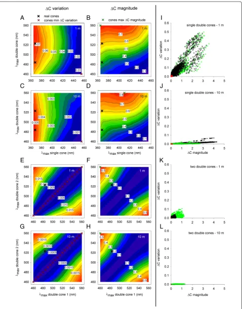
channel formed by one single cone and one double cone located at a depth of 1 m are plotted for various cone pigment pairs in Figure 4A and B, respectively. Calculated values are displayed in the white tags on the isovalue contours across the various pigment combinations. Values rise from blue to red regions on the plots. Figure 4C,D presents findings for the same model channel located at a depth of 10 m. Results for similar analysis of an opponent pair of double cones are plotted in Figure 4E-H. For the opponent channel formed by comparison of one single
cone and one double cone, the maxΔCmag pigment pair
constituted of pigments with λmax that were far apart
(365 and 560 nm for 1 m depth; 410 and 560 for 10 m depth; Figure 4B,D, green X symbols), while the minΔCvar pigment pair constituted of pigments withλmaxthat were
closer together (455 and 460 for both 1 and 10 m depth; Figure 4A,C, red X symbols). Similarly, for the opponent channel formed by comparison of two double cones, the
maxΔCmag pigment pair constituted of pigments with
λmaxthat were far apart (460 and 560 nm for both 1 and
10 m depth), while the minΔCvar pigment pairs consti-tuted of two identical pigments with λmax spanning the
realistic range for double cones (460 to 560 nm), for both 1 and 10 m depth (Figure 4E-H). Thus, theλmaxof the real
pigments inM. zebra(368, 484, and 523 nm; black X sym-bols),and the spectral separation between the pigments,
re-semble those of the maxΔCmag pigments more than they
resemble those of the minΔCvar pigments.
Next, we examined quantitatively how theΔC
magni-tude produced by the actual cone pigments in M. zebra
corresponds to the ΔC magnitudes produced by the
maxΔCmag and minΔCvar pigments. Because of the
large sample size (n = 696 for each of the groups, 87
body patterns × 8 rock substrates), slight differences between treatment groups most often resulted in statisti-cally significant differences between groups (P <0.05). We therefore chose to report observed effect size (that is, η2 values) to allow evaluation of the magnitude of difference between groups. The larger the effect size, the larger is the difference between treatment groups. Unless specified differently,Pfor all comparisons was <0.05.
For the opponent channel formed by one single cone and one double cone (Figure 4I,J),ΔCmagnitude differed between the real (black), minΔCvar (red), and maxΔCmag (green) pigment pairs (RT, df = 3,N= 696 for each group,
η2
= 0.243 and 0.186 for 1 and 10 m depth). Post-hoc
analysis revealed that ΔC magnitude for the minΔCvar
pigment pair was smaller than for either the real pigment pairs (SWS1-Rh2b, df = 1,η2= 0.312 and 0.253 for 1 and
10 m depth; SWS1-Rh2a, df = 1, η2 = 0.362 and 0.289
for 1 and 10 m depth) or the maxΔCmag pigment pair
(df = 1,η2= 0.422 and 0.446 for 1 and 10 m depth). In
pigment pairs differed only slightly (RT, df = 2,η2= 0.027 and 0.005 for 1 and 10 m depth), as did theΔCmagnitude for the real pigment pairs (RT, df = 1, η2 = 0.013 and 0.006 for 1 and 10 m depth). Therefore, theΔCmagnitude
produced by the real and maxΔCmag pigment pairs is
largely similar, but considerably larger than theΔC magni-tude produced by the minΔCvar pigment pair.
For the opponent channel formed by two double cones
(Figure 4K,L), ΔC magnitude differed between the real,
minΔCvar, and maxΔCmag pigment pairs (RT, df = 2,
N= 696 for each group,η2= 0.555 and 0.556 for 1 and 10 m depth).Post-hocanalysis revealed thatΔCmagnitude for the minΔCvar pigment pair was smaller than for either the real pigment pair (Rh2b-Rh2a, df = 1,η2= 0.555 and
0.556 for 1 and 10 m depth) or the maxΔCmag pigment
pair (df = 1,η2= 0.585 and 0.585 for 1 and 10 m depth).
In contrast, ΔC magnitude for the real and maxΔCmag
pigment pairs differed less considerably (RT, df = 1,
η2
= 0.315 and 0.316 for 1 and 10 m depth). Thus, theΔC magnitude produced by the real pigment pair resembles
the ΔC magnitude produced by the maxΔCmag pigment
pair better than it resembles theΔCmagnitude produced by the minΔCvar. Therefore, at both 1 and 10 m depth, the real and maxΔCmag pigment pairs are more effective
than the minΔCvar pigment pair in producing large ΔC
magnitude. These results suggest that the spectral location of pigments inM. zebrais almost optimally tuned to allow
the largest possible ΔC magnitude between fish pattern
and background, as predicted by the contrast theory.
Figure 4I-L allows comparison of the ΔC variation
produced by the real cone pigments in M. zebra with
that produced by the maxΔCmag and minΔCvar pigments. For the opponent channel formed by one single cone and one double cone (Figure 4I,J), the flicker-induced
variation in ΔC differed between the real, minΔCvar,
and maxΔCmag pigment pairs (RT, df = 3,N= 696 for
each group,η2= 0.189 and 0.197 for 1 and 10 m depth). Post-hoc analysis revealed that ΔC variation for the
minΔCvar pigment pair was smaller than for either
the real pigment pairs (SWS1-Rh2b, df = 1, η2= 0.314
and 0.269 for 1 and 10 m depth; SWS1-Rh2a, df = 1,
η2
= 0.319 and 0.263 for 1 and 10 m depth) or the maxΔCmag pigment pair (df = 1,η2= 0.318 and 0.372 for 1 and 10 m depth). However,ΔCvariation for the real and maxΔCmag pigment pairs did not differ significantly at 1 m depth (RT, df = 2,P= 0.257,η2= 0.001), but did differ at 10 m depth (RT, df = 2,P<0.001,η2= 0.071); At both
1 and 10 m depth, ΔC variation for the real pigment
pairs did not differ significantly (RT, df = 1, P = 0.798 andη2= 0.0008 for 1 m depth,P= 0.666 andη2<0.0001 for 10 m depth).
For the opponent channel formed by two double cones (Figure 4K,L), the flicker-induced variation inΔCdiffered
between the real, minΔCvar, and maxΔCmag pigment
pairs (RT, df = 2,N= 696 for each group,η2= 0.458 and 0.563 for 1 and 10 m depth). Post-hoc analysis revealed
that ΔC variation for the minΔCvar pigment pair was
smaller than for either the real pigment pair (Rh2b-Rh2a, df = 1,η2= 0.458 and 0.563 for 1 and 10 m depth) or the maxΔCmag pigment pair (df = 1,η2= 0.488 and 0.598 for 1 and 10 m depth). In contrast,ΔCvariation for the real and maxΔCmag pigment pairs differed less substantially (RT, df = 1,η2= 0.023 and 0.318 for 1 and 10 m depth). Therefore, the real pigment pairs are often slightly more effective than the maxΔCmag pigment pairs in eliminating
the variation in ΔC. Nevertheless, at both 1 and 10 m
depth, the real and maxΔCmag pigment pairs are consid-erably less effective than the minΔCvar pigment pairs in eliminating the variation inΔC. These results suggest that the spectral location of pigments in M. zebra is poorly tuned to allow elimination of temporal fluctuations in the visual signal, in contrast to the prediction of the flicker theory.
Taken together, three lines of evidence suggest that the spectral location of cone pigments inM. zebrahas been shaped as predicted by the contrast theory rather by the flicker theory. These are: (i) similarity in cone spectral
locations between the maxΔCmag pigments and the real
pigments in M. zebra, (ii) greater efficiency of the real
and maxΔCmag pigment pairs in producing large ΔC
magnitude as compared to the minΔCvar pigment pair,
and (iii) lower efficiency of the real and maxΔCmag
(See figure on previous page.)
Figure 4Spectral location of pigments inMetriaclima zebrais tuned to allow large chromatic contrast between fish pattern and background. (A-H)MedianΔCbetween fish pattern and background.ΔCwas modeled for opponent channels that compare the outputs of one single cone and one double cone(A-D), and channels that compare the outputs of two double cones(E-H). The various colors and tags in the contour plots represent different medianΔCvalues. The maxΔCmag pigment pairs comprised pigments withλmaxthat were far apart, and
resembled theλmaxof the real pigments inM. zebra(368, 484, and 523 nm). In contrast, the minΔCvar pigment pairs consisted of pigments with
λmaxthat were closer together. This trend held for both opponent channel types and for both 1 m and 10 m depth.(I-L)Scatterplots illustrating
the relationship betweenΔCmagnitude andΔCvariation for the real (black), minΔCvar (red), and maxΔCmag (green) pigment pairs.ΔC magnitude produced by the real pigment pair resembled theΔCamplitude produced by the maxΔCmag pigment pair better than it resembled theΔCamplitude produced by the minΔCvar. This was observed at both 1 m and 10 m depth, and for both opponent channel types
pigment pairs in eliminating the variation in ΔC, as
compared to the minΔCvar pigment pair. Thus, the
spectral location of pigments in M. zebra is tuned to
produce large ΔC magnitude between fish pattern and
background, and is poorly tuned to allow elimination of temporal fluctuations in the visual signal. That is, the
visual system of M. zebra is tuned as predicted by the
contrast theory rather than by the flicker theory (or by both theories).
Conclusions
Our results show that the amplitude of the light flicker and the distribution of its power across temporal fre-quencies vary across the light spectrum, violating the flicker theory’s first assumption. We examined the effect of the wavelength dependence of light flicker on the out-put of cones and found that, contrary to the prediction of the flicker theory, simple subtraction of the output of one cone class from that of another through opponent interactions would not produce a flicker-free output signal. Moreover, neither fixed low pass filtration nor adjustment of dynamic range of cones would likely to be favored. Thus, although there might be a mechanism by which flicker-free visual signals would be generated under flickering illumination, the likelihood of such a possibility is low. Importantly, even if such generation of a flicker-free visual signal would prove possible, our results show that the temporal frequency of flicker matches the frequency where sensitivity is maximal in a wide range of fish species, suggesting that the flicker may potentially enhance the detection of objects. Thus, there appears to be no real need to eliminate the flicker, because, in contrast to the accepted belief and the second assumption of the flicker theory, the flicker can most likely improve the detection of objects rather than degrade it. The violation of its two critical assumptions suggests little support for the flicker theory as originally formulated. While this alone does not support the contrast theory, comparison of the contrast and flicker theories by means of chromatic contrast modeling under flickering illumination revealed that the visual system of our focal species was tuned as predicted by the contrast theory rather than by the flicker theory. This suggests that the main factor that has tuned the spectral locations of cone pigments is the optimization of visual contrast. Thus, we propose that the contrast theory, stating that multiple cone classes evolved to maximize the visual contrast between objects and backgrounds, is the most parsimonious at present. This result may have important implications for our understanding of the adaptive significance of the number and spectral tuning of cone pigments and the characteristics of retinal networks in vertebrate visual systems.
Methods
Measurement of underwater light flicker
The study was conducted on 21 July 2008 at a near-shore site at Cape Maclear, Nankumba Peninsula, Lake Malawi. The sampling site (14° 01’ 26.42”S 34° 49’ 25.91”E) was located on the southern shore of Thumbi West Island. This site is exposed to wind and wave action [55] and has a rock-sand transition depth of approximately 12 m.
To study the light flicker characteristics, downward and sideward irradiance was measured at a high sampling rate. Irradiance was measured using a thermoelectrically cooled spectroradiometer (QE65000, Ocean Optics, Dunedin, FL, USA) connected to a 30 m optical fiber (ZPK600-30 Ultra-violet–visible, Ocean Optics) that was fitted with a cosine corrector (diameter = 3.9 mm; CC-3-Ultraviolet, Ocean Optics). This diameter of the cosine corrector was expected to accurately capture the irradiance fluctuations at near-surface depths. However, we cannot exclude the possibility of miscapturing fluctuations of small spatial scale, typically encountered at depths smaller than 1 m [22]. The spec-troradiometer employed a 1,024 × 58-element square silicon charge-coupled device (CCD) array, configured with a 25μm slit and a variable blaze wavelength grating
(HC-1, groove density = 300 mm-1, Ocean Optics),
resulting in an effective spectral resolution of 1.9 nm‘Full
Width at Half Maximum’(FWHM) between 200 and 950
nm. The spectroradiometer’s integration time was set to 25 ms (theoretical sampling frequency = 40 Hz) to allow for the highest possible sampling rate while ensuring sufficiently high signal-to-noise ratio. In practice, however, due to a time constant between successive readings, the actual sampling frequency was 17.34 Hz. Thus, 3,000 measurements were saved over 173 s, constituting a measurement time series. The spectroradiometer setup was calibrated for absolute irradiance prior to measurement using a calibrated halogen-deuterium dual light source (200 to 1,000 nm, DH-2000-CAL, Ocean Optics). The optical fiber head was mounted on a 1 m tall tripod, 1, 2, 4, 6, and 10 m below the water surface, and readings were saved on a laptop computer placed on a boat. To prevent shading, the boat was positioned as far as possible from the tripod and never between the tripod and the sun. Irradiance measurements were conducted under clear blue sky, at 12:20 to 14:09 (local time), with solar zenith angles of 46° to 55°, and under light winds of 1.8 m/s.
fiber optic and cosine corrector) for absolute irradiance. Therefore, spectrally-specific differences in the design of the spectroradiometer setup likely had little effect (if any) on the observed wavelength dependence of light flicker.
Although vision is essentially a task of low spectral reso-lution and high temporal resoreso-lution radiance detection, we have chosen to measure irradiance at a relatively low temporal resolution for several reasons. First, we aimed at investigating the wavelength dependence of light flicker, so we chose to sacrifice some temporal resolution while ensuring precise representation of irradiance across the spectrum. Second, we chose to focus on characterization of light flicker at temporal frequencies corresponding to the Fmax of fish;, typically ranging between 2 and 4 Hz
(Figure 3). Third, the power of light flicker typically declines steeply with increasing temporal frequency. For example, the power of light flicker at a frequency of 8.67 Hz (our frequency limit considering a sampling frequency of 17.34 Hz) was reported to be approximately 5 to 200 fold smaller than that at the dominant frequency at depths of 0.86 to 2.84 m [56]. Indeed, to fully capture the highest-frequency irradiance fluctuations, it would be necessary to use a high rate (for example, 1 kHz) radiometric measure-ment system [22]. However, the relatively low frequency of Fmaxin fish as well as the steep decline of light flicker’s
power with increasing frequency, suggest a limited effect of high-frequency irradiance fluctuations on the appearance of objects.
Analysis of amplitude and temporal frequency of light flicker
To standardize the 3,000 readings included in each irradi-ance time series, the noise level (measured with the tip of the cosine corrector blocked) was subtracted from each spectroradiometer reading, and the resulting reading in relative counts was converted into photon irradiance. Wavelengths at which irradiance was lower than 3 × 10¹¹
photons cm2/s/nm were designated as unreliable and
removed from further analysis. To estimate the amplitude of the light flicker, we calculated the CV of each irradiance time series. CV is commonly used in describing the variation in irradiance and radiance flicker [22,34,35,57]. To study the frequency characteristics of the wave-induced light flicker, we calculated the power spectrum of temporal frequencies for each irradiance time series at a light wave-length resolution of 1 nm. Specifically, the discrete Fourier transform (DFT) was calculated for each time series by using the fast Fourier transform (FFT) algorithm, and while applying a Hamming frequency window that is appropriate for analyzing closely spaced sine waves [58]. Additionally, as indices of the distribution of power across frequencies, we calculated the fP50, fP90, fP99 that stand
for the frequencies corresponding to 50, 90, and 99 percent of the cumulative power of the light flicker.
Although dependent on the frequency range examined, the fP indices describe the modulations experienced by an observer reasonably well [40]. Finally, to assess the wave-length dependence of the power distribution of light flicker, we calculated the root mean square error (RMSE) and the normalized RMSE (NRMSE) between the power distribution at 500 and 550 nm. Irradiance at these wavelengths is highest and most reliable, and thus, the calculated RMSE and NRMSE are likely to serve as good estimates for wavelength dependence. NRMSE equaled RMSE divided by the difference between the maximum and minimum power across the spectrum.
Modeling the magnitude and variation of chromatic contrast under flickering illumination
Chromatic contrast modeling was performed following
Kelber et al. [59] and Cummings [60]. The quantum
catch of each cone photoreceptor, Qi, when viewing a
given color patch of the fish was calculated according to:
Qi¼ Z800
300
Rtð ÞEhλ ð ÞAiλ ð ÞTλ ð Þdλ λ ð1Þ
where Rt(λ) is the spectral reflectance of the target
(ranging 0 to 1),Eh(λ) is the normalized sideward
spec-tral irradiance incident on the object (ranging 0 to 1),Ai
(λ) is the normalized absorbance of cone photoreceptori (ranging 0 to 1), and T(λ) is the normalized spectral transmission of the ocular media (ranging 0 to 1). Simi-larly, the quantum catch of each photoreceptor when viewing the background of a rock substrate (the stimulus fish might be viewed against) was calculated using Equa-tion 1 whereRt(λ) was substituted by the spectral
reflect-ance of the substrate, Rb(λ). The absorbance of
photoreceptors was estimated as the empirical absorbance templates of visual pigments given by Govardovskiiet al. [61]. See below detailed procedures for the measurement of spectral reflectance of the body pattern of fish and rock substrate (approximated by diffuse reflectance [62]), and spectral transmission of the ocular media (approximated by the transmission of the lens [63]). The quantum catch of photoreceptors should ideally be estimated using absorbtance rather than absorbance spectra, with the former depending on the transverse specific density of pigments and the outer segment length of photoreceptors. However, transverse specific density and outer segment length data inM. zebra(our focal species) and in African cichlids as a whole is largely unexplored, with the few available reports providing incomplete and contradicting values [64-66]. Thus, photoreceptor quantum catch was estimated using absorbance spectra.
To account for the light adaptation properties of
normalized to the adapting background irradiance by the von Kries coefficients,Ki:
qi¼Ki Qi ð2Þ
TheseKicoefficients were chosen so that the quantum
catches for the adapting irradiance is constant, that is:
Ki¼1= Z800
300
Ehð ÞAiλ ð ÞTλ ð Þdλ λ ð3Þ
whereEhð Þλ is the normalized mean sideward spectral ir-radiance that was assumed to adapt the fish eye, calculated as the time-average of 3,000 consecutive sideward irradi-ance measurements. We modeled two types of opponent channels: (i) a channel that compares the outputs of one single cone and one double cone [Csd], and (ii) a channel
that compares the outputs of two double cones [Cdd]:
Csd¼qs−qd
Cdd¼qd1−qd2 ð4Þ
Thereafter, we calculated the chromatic contrast (ΔC), formed by comparison of the output of a given opponent channel when viewing the body color pattern of fish and the background against which it might be viewed:
ΔC¼Ct−Cb ð5Þ
where Ct and Cb represent the output of a given
opponent channel when viewing the object and the
background, respectively. ΔC amplitude was estimated
as the time average of ΔC over 100 consecutive
high-temporal resolution sideward irradiance measurements (total duration = 6 s), andΔCvariation was estimated as
the standard deviation in ΔC over time. The use of
standard deviation, rather than coefficient of variation,
to estimate the variation in ΔC is appropriate because
the quantum catches of photoreceptors were already normalized to the mean adapting irradiance; this effectively rendered the quantum catches of the different cones to be of the same magnitude.
Measurement of spectral reflectance of the body pattern of fish
Diffuse spectral reflectance of the body pattern of M.
zebra (n = 87) was measured at 1-nm intervals using a spectroradiometer (effective spectral resolution = 2.06 nm FWHM for 200 to 950 nm; USB2000, Ocean Optics) connected to one arm of a 2 m bifurcated optical fiber (BIF600-2 Ultraviolet–visible, Ocean Optics). The other arm of the fiber was connected to a high output light source (200 to 1,000 nm; DH-2000-BAL, Ocean Optics). The common end of the bifurcated fiber was fitted with a flat black reflectance probe that showed a 3 mm diameter tip, cut at an angle of 45°. A measurement of a Spectralon
diffuse reflectance standard (WS-1-SL, Ocean Optics) was taken as 100% reflectance, and a dark measurement was taken as zero reflectance. Fish were immersed in 500 ml water containing 2 ml of 1:10 clove oil:ethanol solution immediately after capture until the fish reached stage III anesthesia [67]. Reflectance was measured at 16 to 23 different points across the submerged fish body of 5 indi-viduals. All experimental and animal care procedures were
approved by Queen’s University Animal Care Committee
under the auspices of the Canadian Council for Animal Care.
Measurement of spectral reflectance of rock substrate
Diffuse spectral reflectance of rock substrate (n= 8) was
measured at a near-shore site in Lake Malawi (14° 00’
58.02” S 34° 48’ 33.29” E) [68]. Rock reflectance was measured using a custom-built probe that included a diving flashlight (mini Q40, Underwater Kinetics, Poway, CA, USA) and a fiber-coupled spectroradiometer (Jaz, Ocean Optics). The tip of the flashlight was fitted with an adaptor that held the optical fiber (QP600-2 Ultravio-let–visible, Ocean Optics) oriented at an angle of 45° to the examined surface. The far side of the adaptor included a ring of black foam that sealed the reflectance probe against the surface examined. A SCUBA diver held the reflectance probe against rock substrates while readings were acquired and saved on a laptop computer in a boat. The irradiance spectrum of the flashlight allowed reliable reflectance measurements between 370 and 800 nm, and the spectroradiometer configuration resulted in an effective spectral resolution of 2.06 nm (FWHM) across this range. A measurement of a Spectralon diffuse reflectance standard was taken as 100% reflectance, and a dark measurement was taken as zero reflectance.
Measurement of spectral transmission of fish lens
Spectral transmission of the fish lens was measured following a protocol described elsewhere [69,70]. Lenses were surgically removed from the eyes and were mounted in a hole that was drilled in a black plastic block fitted inside a standard sample cuvette. Transmission measure-ments between 300 and 750 nm were carried out using a bench-top spectrophotometer (Cary 300; Varian, Palo Alto, CA, USA) and were normalized between 0 and 1. For each fish (n = 3), six to ten transmission measure-ments were acquired from both lenses and averaged.
Statistical analysis
Fmax of fish from different water depth categories and
habitat types did not follow normal distribution (Kolmo-gorov-Smirnov test) and differed in variance (Leven’s test). Thus, to test the effect of water depth and habitat
type on Fmax, we used ANOVA permutation tests, with
categories and habitat types as a test statistic (R package
‘lmPerm’, maximum number of iterations = 50,000, α = 0.05) [71]. Similarly, chromatic contrast (ΔC) between fish pattern and background for the real, minΔCvar, and
maxΔCmag pigment pairs did not follow normal
distri-bution and their variance differed between groups. Thus, permutation tests were used also to test the effect of pig-ment pair onΔCamplitude and variation. To allow evalu-ation of the magnitude of difference inΔCamplitude and variation between pigment pair treatments, effect size was estimated asη2(= sum of squares treatment/sum of squares total). Statistical analysis was performed using R 3.0.0 (The R Foundation for Statistical Computing).
Additional files
Additional file 1:Temporal frequency of light flicker is wavelength dependent across various water depths. (A-D)The frequency distribution of the flicker in downward irradiance at a depth of 2 m (A), 4 m (B), 6 m (C), and 10 m (D) differed across the light spectrum. For clear graphical presentation, the power spectrum of light flicker, normalized to the dominant frequency (1.54 Hz for 2 m, 0.83 Hz for 4 m, 0.80 Hz for 6 m, 0.67 Hz for 10 m) is presented for different wavelengths at 50 nm intervals.(E-G)Cumulative power of wave-induced flicker across wavelengths and water depths. As indices of the distribution of flicker power across temporal frequencies, we calculated the fP50, fP90, and fP99
that stand for the temporal frequencies that correspond to 50, 90, and 99 percent of the cumulative power of wave-induced flicker. fP50, fP90, and
fP99increased toward longer light wavelengths, further supporting the
wavelength dependence of the temporal frequency structure of flicker. Note that deeper in the water column, the irradiance at both ends of the spectrum was too low to be considered reliable (see Methods for criteria for excluding data points); therefore, the spectral range presented narrows with depth.
Additional file 2:Amplitude and temporal frequency of the light flicker in sideward irradiance are wavelength dependent. (A,B)
Examples of light flicker time series of sideward irradiance at 1 m depth and light wavelengths of 400 and 600 nm. The amplitude of the light flicker at 600 nm is larger than at 400 nm.(C)The amplitude of light flicker in sideward irradiance decreased with growing water depth, and increased monotonically toward longer light wavelengths. The ratio between the amplitude at the longest and shortest wavelengths did not vary considerably across depths, and ranged between 2.26 and 2.79 (presented next to each spectrum).(D)The frequency distribution of the flicker at a depth of 1 m differed across the light spectrum. The power spectrum of light flicker, normalized to the dominant frequency (1.69 Hz), is presented for different wavelengths at 50 nm intervals. The frequency distribution of flicker at 2, 4, 6, and 10 m depth also differed between wavelengths (not presented).(E)The frequency distribution of light flicker at 500 nm differed across water depths, with the dominant frequency (1 m, 1.69 Hz; 2 m, 1.30 Hz; 4 m, 0.83 Hz; 6 m, 0.78 Hz; 10 m, 0.59 Hz) and the relative power at high frequencies decreasing with growing depth.(F)The wavelength dependence of light flicker became weaker with growing depth.
Additional file 3:Compilation of critical fusion frequency (CFF) and the frequency at which maximum contrast sensitivity is attained (Fmax, estimated as 15% of CFF) in fish.Frequencies are given in Hz. Additional file 4:Comparison between the frequency of light flicker in downward irradiance and two realistic estimates of Fmax.
Fmaxwas estimated as either 10%(A,B)or 20%(C,D)of CFF. (A,C) The
distribution of Fmaxvalues across frequency corresponded well to the
power spectrum of flicker across depths. Note, however, that estimation of Fmaxas 20% of CFF resulted in Fmaxvalues that often exceeded the
sampling frequency limit of light flicker. Depicted power spectrum
(shaded gray) represents the envelope of flicker power across the 1 m and 10 m depth range. (B,D) Comparison between the cumulative power of the flicker and Fmaxfor dim and bright stimuli (closed circles).
Conventions for the indices of the distribution of power of flicker across frequencies (fP50, fP90, and fP99), plot specifications, and species included
in the analysis are the same as in Figure 3A,B. For estimation of Fmaxas
10% of CFF, the median Fmaxequaled 1.2 and 2.3 Hz, for dim and bright
stimuli, respectively (open circle; red error bars represent the 25th and 75th percentiles). The median Fmaxfor dim and bright stimuli matched
the frequency below which approximately 50% of the cumulative power of flicker was found at 1 m depth. For estimation of Fmaxas 20% of CFF,
the median Fmaxequaled 2.4 and 4.6 Hz, for dim and bright stimuli,
respectively. The median Fmaxfor dim and bright stimuli matched the
frequency below which between 50% and 90% of the cumulative power of flicker was found at 1 m depth. For both Fmaxestimates, the median
Fmaxfor dim and bright stimuli matched the frequency below which 99%
of the cumulative power at 10 m depth was found.
Additional file 5:Spectra used for chromatic contrast modelling.
(A,B)A total of 100 spectra of sideward irradiance at a water depth of 1 m (A) and 10 m (B). These spectra were taken as the irradiance that illuminated the stimulus fish and the vertical rock substrate.(C,D)Mean spectral sideward irradiance at a depth of 1 m (C) and 10 m (D) that was taken as the irradiance that adapted the viewer fish eye.(E)Spectral reflectance of the body pattern of fish (n= 87).(F)Spectral reflectance of diverse rock substrates (n= 8).(G)Spectral transmission of the lens in Metriaclima zebra.(H)Spectral absorbance templates for visual pigments of A1chromophore constructed based on the cone pigments typically found
in adultM. zebra: a single cone-occupying pigment (SWS1,λmax= 368 nm)
and two double cones-occupying pigments (Rh2b,λmax= 484 nm; Rh2a,
λmax= 523 nm). For graphical presentation only, each of the spectra
presented in (A-F) was normalized by its norm.
Competing interests
The authors declare that they have no competing interests.
Authors’contributions
SS conceived and designed the study, analyzed the data, and wrote the manuscript; SS and CWH performed all the experiments. Both authors have read and approved the final manuscript.
Acknowledgements
We thank James McIlwain, David Berson and Daryl Parkyn for comments on the manuscript, and Suzanne Gray for assistance with underwater light flicker measurements. This research was supported by a Natural Sciences and Engineering Research Council of Canada (NSERC) Discovery Grant (106102– 07), NSERC Research Tools and Instrumentation Grant (359714–2008), Canada Foundation for Innovation, Ontario Innovation Trust (202821), and the Canada Research Chair Program to CWH. SS was supported by a Vanier Canada Graduate Scholarship from NSERC.
Author details
1Department of Biology, Queen’s University, Kingston, Ontario K7L 3N6,
Canada.2Centre for Neuroscience Studies, Queen’s University, Kingston, Ontario K7L 3N6, Canada.
Received: 10 June 2013 Accepted: 27 June 2013 Published: 4 July 2013
References
1. Bowmaker JK:Evolution of vertebrate visual pigments.Vision Res2008, 48:2022–2041.
2. Hou XG, Aldridge RJ, Siveter DJ, Feng XH:New evidence on the anatomy and phylogeny of the earliest vertebrates.P Roy Soc B-Biol Sci2002, 269:1865–1869.
3. Shu DG, Morris SC, Han J, Zhang ZF, Yasui K, Janvier P, Chen L, Zhang XL, Liu JN, Li Y, Liu HQ:Head and backbone of the Early Cambrian vertebrate Haikouichthys.Nature2003,421:526–529.
5. Collin SP, Trezise AEO:The origins of colour vision in vertebrates.Clin Exp Optom2004,87:217–223.
6. Collin SP, Davies WL, Hart NS, Hunt DM:The evolution of early vertebrate photoreceptors.Philos Trans R Soc Lond B2009,364:2925–2940. 7. Hart NS, Lisney TJ, Marshall NJ, Collin SP:Multiple cone visual pigments
and the potential for trichromatic colour vision in two species of elasmobranch.J Exp Biol2004,207:4587–4594.
8. Theiss SM, Lisney TJ, Collin SP, Hart NS:Colour vision and visual ecology of the blue-spotted maskray,Dasyatis kuhliiMuller & Henle, 1814.J Comp Physiol A2007,193:67–79.
9. Davies WL, Carvalho LS, Tay B-H, Brenner S, Hunt DM, Venkatesh B:Into the blue: gene duplication and loss underlie color vision adaptations in a deep-sea chimaera, the elephant sharkCallorhinchus milii.Genome Res 2009,19:415–426.
10. Yokoyama S, Yokoyama R:Adaptive evolution of photoreceptors and visual pigments in vertebrates.Annu Rev Ecol Syst1996,27:543–567. 11. Walker KR, Laporte LF:Congruent fossil communities from Ordovician and
Devonian carbonates of New York.J Paleontol1970,44:928–944. 12. Chang BS, Crandall KA, Carulli JP, Hartl DL:Opsin phylogeny and evolution:
a model for blue shifts in wavelength regulation.Mol Phylogen Evol1995, 4:31–43.
13. McFarland WN, Munz FW:Evolution of photopic visual pigments in fishes III.Vision Res1975,15:1071–1080.
14. Munz FW, McFarland WN:Evolutionary adaptations of fishes to the photic environment.InHandbook of Sensory Physiology. Volume VII/5.Edited by Crescitelli F. Berlin, Germany: Springer-Verlag; 1977:193–274.
15. Neumeyer C:Evolution of color vision.InVision and Visual Dysfunction. Edited by Cronly-Dillon JR, Gregory RL. London, UK: Macmillan, Houndsmills; 1991:282–305.
16. Osorio D, Vorobyev M:A review of the evolution of animal colour vision and visual communication signals.Vision Res2008,48:2042–2051. 17. Sabbah S, Troje NF, Gray SM, Hawryshyn CW:High complexity of aquatic
irradiance may have driven the evolution of four-dimensional colour vision in shallow-water fish.J Exp Biol2013,216:1670–1682. 18. Spady TC, Parry JWL, Robinson PR, Hunt DM, Bowmaker JK, Carleton KL:
Evolution of the cichlid visual palette through ontogenetic subfunctionalization of the opsin gene arrays.Mol Biol Evol2006, 23:1538–1547.
19. Ward MN, Churcher AM, Dick KJ, Laver CRJ, Owens GL, Polack MD, Ward PR, Breden F, Taylor JS:The molecular basis of color vision in colorful fish: four long wave-sensitive (LWS) opsins in guppies (Poecilia reticulata) are defined by amino acid substitutions at key functional sites.BMC Evol Biol 2008,8:210.
20. Yokoyama S:Molecular evolution of vertebrate visual pigments.Prog Retin Eye Res2000,19:385–419.
21. Maximov VV:Environmental factors which may have led to the appearance of colour vision.Philos Trans R Soc Lond B2000, 355:1239–1242.
22. Darecki M, Stramski D, Sokolski M:Measurements of high-frequency light fluctuations induced by sea surface waves with an underwater porcupine radiometer system.J Geophys Res2011,116:C00h09. 23. Schenck H:On the focusing of sunlight by ocean waves.J Opt Soc Am
1957,47:653–657.
24. Snyder RL, Dera J:Wave-induced light-field fluctuations in the sea.J Opt Soc Am1970,6:1072–1079.
25. Stramski D, Dera J:On the mechanism for producing flashing light under a wind-disturbed water surface.Oceanologia1988,25:5–21.
26. Kamermans M, Spekreijse H:Spectral behavior of cone-driven horizontal cells in teleost retina.Prog Retin Eye Res1995,14:313–360.
27. Svaetichin G, MacNichol EF:Retinal mechanisms for chromatic and achromatic vision.Ann N Y Acad Sci1958,74:385–404.
28. Kaneko A, Tachibana M:Retinal bipolar cells with double colour-opponent receptive fields.Nature1981,293:220–222.
29. Kaneko A, Tachibana M:Double color-opponent receptive fields of carp bipolar cells.Vision Res1983,23:381–388.
30. Daw NW:Colour-coded ganglion cells in the goldfish retina: extension of their receptive fields by means of new stimuli.J Physiol (Lond)1968, 197:567–592.
31. Fritzsch B, Collin SP:Dendritic distribution of two populations of ganglion-cells and retinopetal fibers in the retina of the silver lamprey (Ichthyomyzon unicuspis).Vis Neurosci1990,4:533–545.
32. Reichenbach A, Robinson SR:Phylogenetic constraints on retinal organisation and development.Prog Retin Eye Res1995,15:139–171. 33. Holmberg K:The cyclostome retina.InHandbook of Sensory Physiology. Volume
VII/5.Edited by Crescitelli F. Berlin, Germany: Springer-Verlag; 1977:47–66. 34. Stramska M, Dickey TD:Short-term variability of the underwater light field
in the oligotrophic ocean in response to surface waves and clouds. Deep-Sea Res I1998,45:1393–1410.
35. Sabbah S, Gray SM, Hawryshyn CW:Radiance fluctuations induced by surface waves can enhance the appearance of underwater objects. Limnol Oceanogr2012,57:1025–1041.
36. Parry JWL, Carleton KL, Spady T, Carboo A, Hunt DM, Bowmaker JK:Mix and match color vision: tuning spectral sensitivity by differential opsin gene expression in Lake Malawi cichlids.Curr Biol2005,15:1734–1739. 37. Riggs LA, Ratliff F, Cornsweet JC, Cornsweet TN:The disappearance of
steadily fixated visual test objects.J Opt Soc Am1953,43:495–501. 38. Kelly DH:Motion and vision. 2. Stabilized spatio-temporal threshold
surface.J Opt Soc Am1979,69:1340–1349.
39. Loew E, McFarland WN:The underwater visual environment.InThe Visual System of Fish.Edited by Douglas R, Djamgoz MBA. London, UK: Chapman & Hall; 1990:1–43.
40. McFarland WN, Loew ER:Wave produced changes in underwater light and their relations to vision.Environ Biol Fishes1983,8:173–184. 41. Bilotta J, Lynd FM, Powers MK:Effects of mean luminance on goldfish
temporal contrast sensitivity.Vision Res1998,38:55–59.
42. Kelly DH:Theory of flicker and transient responses. 1. Uniform fields. J Opt Soc Am1971,61:537–546.
43. Kelly DH:Diffusion model of linear flicker responses.J Opt Soc Am1969, 59:1665–1670.
44. Watson AB:Temporal sensitivity.InHandbook of Perception and Human Performance. Volume 1.Edited by Boff KR, Kaufman L, Thomas JP. New York, NY: John Wiley and Sons; 1986:1–43.
45. Roufs JAJ, Blommaert FJJ:Temporal impulse and step responses of the human eye obtained psychphysically by means of a drift-correcting pertubation technique.Vision Res1981,21:1203–1221.
46. de Lange H:Research into the dynamic nature of the human fovea-cortex systems with intermittent and modulated light. I. Attenuation
characteristics with white and colored light.J Opt Soc Am1958,48:777–784. 47. Kelly DH:Visual responses to time-depebdent stimuli. I. Amplitude
sensitivity measurements.J Opt Soc Am1961,51:422–429.
48. Robson JG:Spatial and temporal contrast-sensitivity functions of visual system.J Opt Soc Am1966,56:1141–1142.
49. Basolo AL:Female preference predates the evolution of the sword in swordtail fish.Science1990,250:808–810.
50. Smith AR, van Staaden MJ, Carleton KL:An evaluation of the role of sensory drive in the evolution of lake Malawi cichlid fishes.Int J Evol Biol 2012,2012:647420.
51. Sabbah S, Lamela Laria R, Gray SM, Hawryshyn CW:Functional diversity in the color vision of cichlid fishes.BMC Biol2010,8:133.
52. Carleton KL:Cichlid fish visual systems: mechanisms of spectral tuning. Integr Zool2009,4:75–86.
53. Carleton KL, Spady TC, Streelman JT, Kidd MR, McFarland WN, Loew ER: Visual sensitivities tuned by heterochronic shifts in opsin gene expression.BMC Biol2008,6:22.
54. Hofmann CM, O’Quin KE, Marshall NJ, Cronin TW, Seehausen O, Carleton KL: The eyes have it: regulatory and structural changes both underlie cichlid visual pigment diversity.PLoS Biol2009,7:e1000266.
55. Ribbink AJ, Marsh BA, Marsh AC, Ribbink AC, Sharp BJ:A preliminary survey of the cichlid fishes of rocky habitats in Lake Malawi.S Afr J Zool1983, 18:149–310.
56. You Y, Stramski D, Darecki M, Kattawar GW:Modeling of wave-induced irradiance fluctuations at near-surface depths in the ocean: a comparison with measurements.Appl Opt2010,49:1041–1053. 57. Gernez P, Antoine D:Field characterization of wave-induced underwater
light field fluctuations.J Geophys Res2009,114:C06025.
58. Oppenheim AV, Schafer RW:Discrete-time Signal Processing.2nd edition. Upper Saddle River, NJ: Prentice-Hall; 1999.
59. Kelber A, Vorobyev M, Osorio D:Animal colour vision - behavioural tests and physiological concepts.Biol Rev Camb Philos Soc2003,78:81–118. 60. Cummings ME:Modelling divergence in luminance and chromatic
61. Govardovskii VI, Fyhrquist N, Reuter T, Kuzmin DG, Donner K:In search of the visual pigment template.Vis Neurosci2000,17:509–528.
62. Dalton BE, Cronin TW, Marshall NJ, Carleton KL:The fish eye view: are cichlids conspicuous?J Exp Biol2010,213:2243–2255.
63. Losey GS, McFarland WN, Loew ER, Zamzow JP, Nelson PA, Marshall NJ: Visual biology of Hawaiian coral reef fishes, I. Ocular transmission and visual pigments.Copeia2003,2003:433–454.
64. Braekevelt CR, Smith SA, Smith BJ:Photoreceptor fine structure in
Oreochromis niloticusL. (Cichlidae; Teleostei) in light- and dark-adaptation.Anat Rec1998,252:453–461.
65. Carleton KL, Harosi FI, Kocher TD:Visual pigments of African cichlid fishes: evidence for ultraviolet vision from microspectrophotometry and DNA sequences.Vision Res2000,40:879–890.
66. Fernald RD, Liebman PA:Visual receptor pigments in the African cichlid fish,Haplochromis burtoni.Vision Res1980,20:857–864.
67. Jolly DW, Bucke D, Mawdesle LE:Anesthesia of fish.Vet Rec1972, 91:424–426.
68. Sabbah S, Gray SM, Boss ES, Fraser JM, Zatha R, Hawryshyn CW:The underwater photic environment of Cape Maclear, Lake Malawi: comparison between rock- and sand-bottom habitats and implications for cichlid fish vision.J Exp Biol2011,214:487–500.
69. Lisney TJ, Studd E, Hawryshyn CW:Electrophysiological assessment of spectral sensitivity in adult Nile tilapiaOreochromis niloticus: evidence for violet sensitivity.J Exp Biol2010,213:1453–1463.
70. Sabbah S, Hui J, Hauser FE, Nelson WA, Hawryshyn CW:Ontogeny in the visual system of Nile tilapia.J Exp Biol2012,215:2684–2695.
71. Edgington ES:Randomization Tests.New York: Marcel-Dekker; 1995.
doi:10.1186/1741-7007-11-77
Cite this article as:Sabbah and Hawryshyn:What has driven the evolution of multiple cone classes in visual systems: object contrast enhancement or light flicker elimination?BMC Biology201311:77.
Submit your next manuscript to BioMed Central and take full advantage of:
• Convenient online submission
• Thorough peer review
• No space constraints or color figure charges
• Immediate publication on acceptance
• Inclusion in PubMed, CAS, Scopus and Google Scholar
• Research which is freely available for redistribution