An analysis of changes
to transient processes
occurring in trunk
pipelines as a result of
introducing drag-reducing
agents
by Dr V.V.Zholobov, D.I. Varybok*, and D.V.Egorov
Pipeline Transport Institute (PTI, LLC), Moscow, Russian
Federation
T
HE HYDROBLOW PHENOMENON occurs when there isa sudden change in the flow rate of transported fluids. A shock wave, which is formed at the place where the flow
changes, travels along the pipeline, interacting with equipment and
dying down according to a specific law. It is rather labour-intensive,
and takes a considerable amount of time, numerically to analyse the wave processes in order to draw up maximum-pressure diagrams. A substantial quantity of information obtained from numerical calculation using difference schemes is as yet unused. The aim of
the present study is to find an analytical approach for constructing a
maximum-pressure-envelope curve.
The authors assume that in arbitrary reference conditions, at the
formation stage, a laminar flow regime is found behind the shock
wave. In this case, it can be established that the problem of attenuation of the pressure-surge amplitude in a weakly compressible, viscous liquid has an explicitly analytical solution.
Parametric analysis has shown that, where the regimes before and after the shock wave are combined arbitrarily, the solution has an advantage over the available relationships in terms of accurate wave-amplitude representation. In addition, it allows a method and formulas to be obtained for the conversion of wave parameters in liquids which do and do not contain drag-reducing agents (DRAs).
Based on conversion formulas, parametric analysis was carried out for the impact of DRAs on hydroblow wave amplitudes. It was
confirmed that, all other conditions being equal, the intensity of wave processes is higher in the fluids containing DRAs. This situation
dictates the necessity of adjusting protection parameters for such
fluids in particular.
An approximate analytical dependence was constructed for the pressure distribution behind the pressure-surge front. Combined with
Corresponding author’s contact details: email: varibokdi@niitnn.
the correlation between wave amplitude and conversion formulas, this means the analytic formulation of a maximum-pressure-envelope curve is possible. Applying this approach when performing ‘mass’ parametric calculations means that, using preliminary analysis, options that are of no importance for safe pipeline operation can be excluded from consideration.
Key words: wave amplitude, shock pressure, attenuation, additives, analytical solution, conversion formula
D
RAG REDUCING AGENTSARE conventionally used to increase the throughput capacity of a pipeline; alternatively, they are used to reduce the operating pressure when pumping. The reduction in operating pressure in turn leads to decreased energy expenditure for work overcoming flow resistance during pipeline transport. In both cases, the aim is achieved by reducing the flow resistance in the pipeline.
Mathematically, the difference between the equations describing isothermal one-dimensional flow in liquids with and without additives lies in the magnitude of shearing stress on the pipeline wall. A discontinuity in shear stress occurs at the interface between the two liquids, which moves with the velocity of the liquid. This means that the interface has all properties of a weak contact discontinuity. Under the impact of the shock wave, this discontinuity does not generate a reflected shock wave.
The weak discontinuity (a derivative discontinuity) is reflected at the interface location by a dogleg in the hydro-slope line. The wave processes in a liquid containing a DRA and in a liquid without additives differ in the degree of wave attenuation. In a fluid containing DRAs, where other conditions are equal, the wave process will occur more intensively.
The degree of shock-wave attenuation in a long pipeline depends on many of its parameters and on the properties of the pumped fluid. Describing them in real terms is an important, expensive, and sizeable task. Many methods of assessing the state of trunk oil and petroleum-product pipelines are based on the
principle of recording wave disturbances. Thanks to systems of dispatcher control and management, quantitative characteristics can be obtained for the behaviour of distributed hydraulic parameters in extended systems under real conditions. This situation makes it possible to improve the quality of mathematical modelling for these systems and, in many cases, to replace full-scale experiments with numerical ones.
A theoretical solution to the problem of shock-wave-amplitude attenuation in pipelines was obtained before this study [1]. It will be discussed briefly in this article, and then numerical-calculation data will be analysed and compared using a difference scheme and partial analytic dependences (both already available and obtained in the course of this study).
The numerical analysis of DRA impact on wave processes in real oil and oil-product pipelines is associated with the necessity of considering a large number of variants, and is connected with a significant amount of computational work. A method and an analytical tool must be obtained which will make it possible to quickly and easily give a reliable estimate of the change to wave-attenuation magnitude, when the properties of the pumped liquid change (depending on the presence or absence of DRAs). Particular analytical solutions allowed such a method to be formulated.
∆P ∆P Q cd x
= ⋅ −
0 exp 0 03
λ
π (1)
where
DP = the hydroblow wave amplitude
DP0 = the initial hydroblow wave amplitude
c = the speed of sound according to Zhukovsky
Q0 = the liquid volumetric flow rate ahead of the wave front
d = the internal diameter of the pipeline
l0 = the hydraulic resistance factor ahead of the wave front
|x| = the distance travelled by the wave front from its initial position
It should be kept in mind this relationship is obtained for laminar-flow regimes (ahead of the wave front and behind it), for which DRAs are deliberately not used (as they have zero efficiency). However, it may be of interest to assess the possibility of using Equn 1 for turbulent-flow regimes, including for liquids containing DRAs. Parameters relating to liquids with an additive and without an additive will be denoted respectively as superscript A and Ο. Wave propagation will now be examined for liquids with an additive and without an additive, given identical flow characteristics, both ahead of the hydroblow wave front, and behind it. According to Zhukovsky’s formula, the identical nature of flows in the hydroblow wave by flow rate is guaranteed under the condition ∆PA =∆P PO
(
A ≠PO)
.Taking into account the condition of liquid flow identity according to the flow rate, the following relationship results from Equn 1:
| | (xO ) | | x ,
Q A Q
A
= 1− ×
(
1−)
= 00
ψ ψ λ
λΟ
where
yQ is the hydraulic efficiency of an additive at a constant flow rate [3]
xOand xA are two points ensuring parity
∆P xA( )A =∆P xO( )O .
Taking into account the previous relationship, equalities can be obtained for recalculating the hydroblow wave amplitude depending on the distance travelled by the wave front and using Ewun 2 (below).
Therefore, where calculations for one of the liquids are available, the attenuation of the waves’ amplitude in another liquid can be formally recalculated using relationships Equn 2. It can be clearly seen that where relationship Equn 1 is applicable for turbulent regimes, it could also be used both for estimating the calculated values of DPA or DPO, for an experimental assessment of DRA efficiency. To do this, it is sufficient to generate a wave of controlled amplitude at some point in the pipeline with moving liquid, and to measure the amplitude of the same wave at another point, which is located at distance L from the first one. The required result gives the relationship shwn in Equn 3 (below).
When using Equn 3, it should be kept in mind that L = 0 is a singular point. Since transient regimes are closely related to wave processes, the method for determining the hydraulic efficiency of an additive using Equn 3 may prove to be preferable for calculating unsteady movement in a liquid containing DRAs. This can be done using software packages (SPs), which use simplified versions of balance ratios for hydro-elasticity. The main weakness of this method is the necessity of generating hydroblow itself.
∆PA x ∆P xΟ ∆P xΟ ∆PA x
Q Q
( )
=( )
=−
(
)
−
( (1 ));
1
ψ
ψ
ψ π
λ
Q A A A
cd Q L
= −1 3
(
)
−(
)
0 0
ln P∆ 0 V ln P∆ V
(2)
Since Zhukovsky’s formula is formally applicable for the depressurization shock wave as well, it can also be used for experimental assessment of DRA efficiency. It should be kept in mind that the actual depressurization wave is a centred wave, and this must be taken into account when assessing the range of applicability.
Numerical experiment
The level of inaccuracy when analytical relationships Equns 1 or 3 are used in a turbulent-flow regime can be estimated using existing SPs when applying numerical calculations of transient processes. These SPs use the same mathematical flow model on which the indicated ratios are based. In this case, instead of the empirical value for wave amplitude, it is sufficient to use the virtual wave amplitude obtained using SP.
The validity of applying Equns 1 and 2 can be judged from Fig.1, which shows the results of the transient process numerical calculation in a model horizontal pipeline using the Cassandra SP. For this calculation, the following initial data were selected:
Dnominal = 1 m L = 105 m
Q0 = Q0A = 1.75 m3/s
r = 850 kg/m3
ν = 10 cSt
Ψ = 0.272327
Two variants were considered: the flow of a liquid without an additive, and the flow of a liquid containing DRAs in a concentration providing the level of efficiency indicated above. The calculated efficiency (which follows from Equn 3) depends on the wave front coordinates. As follows from the calculation results shown in Fig.1, the relationship in Equn 3 for turbulent flows in pipelines can give an error level of more than 9%. In other words, the result following from the assumptionλ0 0u =λΦ Φu (author’s notations [2] are retained) is rather rough for turbulent flow regimes and must be adjusted. These adjustments can be made in two ways:
• the relationship in Equn 1 is preserved and a selective choice is made for the point corresponding to target value Ψ
• an analogue of relationship in Equn 1 is presented without the assumption λ0 0u =λΦ Φu .
In view of its greater generality, the second option is further considered as part of a simplified model for the flow of an incompressible viscous liquid, formulated in Ref.1, which subsequently found wide application in the hydraulics of pipeline liquid transportation.
Refined analytical solution
The model given in Ref.1, according to the author, is a generalization of Zhukovsky’s model [4] for viscous liquids. For an ideal liquid, a simplified version of Charny’s model [1, p. 20, Equn 1.28] has the form:
−∂
∂ =
∂ ∂ −∂
∂ = ∂
∂ =
p x
u t p
t c
u x
ρ
ρ ρ
2 ; const (4)
where p, r, and u are the pressure, density and velocity of the liquid, respectively.
Zhukovsky’s classic equations for the problem of hydraulic impact [4], in contrast to the equations Equns 4 above, also contain the convection components
Fig.1. Efficiency distribution of the DRA:
of the total time derivatives for functions p and w:
−∂ ∂ =
∂ ∂ +
∂ ∂
− ∂ ∂ +
∂ ∂
=
∂ ∂
p x
w t w wx p
t w px c
w x
ρ
ρ
0
2 0
(5)
An approximate analytical solution of the system in Equns 5 is used to study the phenomenon of hydraulic impact in [4], and is nevertheless an exact solution to Equns 4. The latter situation, apparently, served as the basis for the previously mentioned author’s assertion [1]. The main weakness of Equns 4 is that, unlike Equns 5, they do not reflect the law of conservation of mass for the transported fluid. Accordingly, in the study of arbitrary one-dimensional non-stationary processes, the system of equations given in works [5, 6] (Equns 6, below) is preferable to Equns 4. In Equns 6:
Qp = puf = the mass flow rate Kg = the liquid compression module E = the module of pipe wall material
elasticity
δ = pipe wall thickness
f = the internal area of a pipe cross-section
χ = the wetted perimeter of a pipe cross-section
(β – 1) is the Coriolis coefficient (a correction for unevenness in the velocity profile)
z = the geodesic mark of the lower surface of the pipeline
The values of velocity u+ and pressure p+ behind the shock wave front as a part of the model in Equn 4 (applicable to the hydroblow problem) are related to the same parameters u– and p– ahead of the wave front by Zhukovsky’s relationship shown in Equn 7 (below).:
The term dx/dt =-c in the following condition is satisfied:
d
dt p cu
c d
u
du
+− + + +
(
)
==
( )
=
ρ λ ρ
λ λ
ν
2
2 Re
Re
(8)
For the liquid flow ahead of the wave front, the following equation is used:
d
dxp d
u − = −λ−1 ρ −
2
2
Re-writing the last equation considering Equn 8, the following is obtained:
d dtp
c d
u − = −λ− ρ −2
2 (9)
Through simple transformations of Equns 7, 8 and 9, the following equation (Equn 10 - see over) can be obtained for the velocity of the liquid behind the shock wave front and velocity surge.
−∂ ∂ =
∂ ∂ ∂
∂ +
∂
∂
(
)
= −∂
∂
(
+)
−=
p t
c f
Q x Q
t x Q u f x p g z u
2 0
0 0 0 2 0
8
1 ρ
ρ
ρ
β ρ λρ χ
ρ ρ ++ −
= + −
p p K
f f d p p
E
g
0
0 1 δ 0
∆ p= +−p− =ρc u u( −+ +)= −ρc U∆ ,ρ ρ= −
(6)
d dtu
u u
d d U u
d
dt U
u U u
d + − − + + + − − − + − = − =
(
+)
( )
= −(
+)
λ λ ν λ λ 2 2 2 2 4 4 Re ∆ ∆ ∆ (10)Since the right-hand side depends only on the required function, u+ and DU can be calculated from Equn 10:
t d
u u du
t d
u U u d U
u = − = −
(
+)
( )
− − + + + − − + − + −∫
4 4 2 2 0 2 2 λ λ λ λ ∆ ∆ uu U −∫
∆ (11)The implied time-dependence of the velocity and of the liquid velocity surge behind the wave front is given in Equn 11. When calculating the value of DP, instead of Equn 7 it is appropriate to use the implied relationship obtained by analogy with velocity surge DU, given by Equn 12 (below).
Taking into account that the independent variables on the wave front are linked by the relationship x=–ct, Equn 12 can be presented as shown in Equn 12 (below).
Thus, for an entirely turbulent-flow regime, and the arbitrary relationship of the hydraulic resistance factor to the Reynolds number, it is necessary to use the implied relationship Equn 13 instead of Equn 1. Since the aim of this paper is to estimate the maximum absolute values of pressure which are reached when the initial stationary flow undergoes maximum deceleration, it is appropriate to single-out from relationship Equn 13 the case characterized by a turbulent-flow regime ahead of the hydroblow wave front (Re– > Re
cr) and by a laminar-flow regime
behind the hydroblow wave front (Re+ <
Recr).
Taking the integral of Equn 13, in this case, and the solution is written as shown in Equn 14 (below).
Equation 14 gives the distribution of hydroblow wave amplitude where there is a sudden shut-off in the pipeline. It is a generalization of Equn 1 for a case of turbulent flow ahead of the wave front. It is easy to see that a similar relationship (Equn 14) may also be obtained for partial deceleration and reversed flow. For this, it is only necessary to take into account that the value of u+ at the moment of hydraulic surge formation is not zero. The domain of applicability of Equn 14 is given by the inequality Re+ < Recr, which can be represented using Equn 11 as follows:
t d
c u
P
c u d P
d c cu P = − −
( )
= ⋅ + − − − − + −∫
4 2 2
1 ρ λ ρ λ ρ ρ ∆ ∆ ∆
Re uu P
c −−
(
∆)
¼
x d u
c u d P
P
cu P = − − ( )
=( )
+ − − − − + + −∫
4 2 2
1 ρ λ ρ λ λ λ ρ
∆
∆ ∆ Re∆P cu Q
d c x
0
4
2 2 0
< ≤
=
−
=
− − + +
+
∫
x x
x dc
u u du
u d
kp kp
u
kp kp
kp
λ λ
νRe
(15)
Expanding this equation, the following is obtained:
xkp = −d c − kp
− −
2
2
16 1
64
νln λ
Re
Re (16)
Analysis of Equn 16 shows that in real conditions, the value of xcr is much smaller than the distance between stations. Assuming, for example, that the flow of the fluid ahead of the hydroblow front occurs in the Blasius regime (Re- > 3000) with initial data: d = 1 m; c = 103 m; ν = 10 cSt; u– = 1 m/s, the following is obtained: xcr = 6748 m. This is the basis for theoretical consideration of other (complementary) flow options where there is a sudden shut-off in a real pipeline.
Equation 14 in the area of its applicability given by Equns 15 and 16 is an exact analytical solution for the shock-wave amplitude in the Charnoy model with non-linear friction, and this allows it to be used as an analytical test in comparative analyses of various versions of difference schemes.
Formulas for calculating hydroblow-wave amplitude, taking into account attenuation because of hydraulic losses along the length of the pipeline section and flow by-pass through a pump station, are also available in Refs 7-11.
Using the notations accepted in this article, the relationship given Refs 7-9 is represented as:
∆P c U∆ K x
L
K u L
dc
L
L
=
( )
× −
= − − ρ
λ
0
1 5
2
1 5
exp .
.
(17)
The following relationship is given in Refs 8 and 11:
∆P c U∆ Q
d cx
=
( )
⋅ −
− −
ρ λ
π
0 3
2 3
exp
(18) where
L = the length of the pipeline section
DU(0) is the amplitude of the velocity wave in the place of formation
As has already been noted, Equn 14, in contrast to Eqns 17 and 18, is an exact solution (as a consequence of the initial system of partial-derivative differential equations). It can be used as an analytical test for numerical calculation of the initial system of equations.
The distinctive feature of Equn 14 compared to similar relationships is the difference in flow regimes ahead of the shock wave front and behind it.
Illustrative calculations
A graphic illustration of estimations for hydroblow wave amplitude attenuation using the relationships in Equns 14, 17, 18, and the Cassandra software package is shown in Fig.2.
Calculations have shown that the numerical solution for liquid pressure at the shock wave front is almost identical (with deviation less than 1%)
Fig. 2 The amplitude of the shock wave spreading upstream.
red line: numerically using the characteristic method green line: using Equn 1 blue line: using Equn 14 purple line: using Equn
17 yellow line: using Equn
to the analytical solution (Equn 14). Relationships in Equns 1, 17, and 18 deviate by 2-4.2 %.
The DRA influence can be analysed using Equn 13 similarly to the analysis using Equn 1. With the help of Equn 13, the applicability limits of the simplified relationship in Equn 1 can be defined more precisely and, in addition, numerical methods of calculation can be tested for an arbitrary flow regime.
When using Equn 14 instead of Equn 1, Equn 3 is adjusted as follows:
ψ ρ
ρ
Q V
A V
P cu
P cu
= − −
−
−
−
1 ∆
∆ (19)
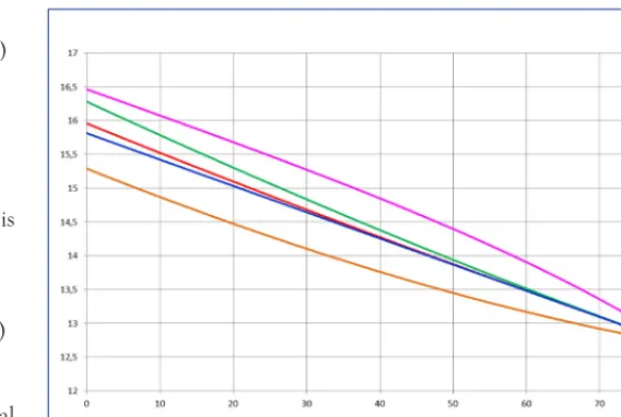
The validity of using Equn 19 for experimental calculation of additive efficiency can be seen in Fig.3, which presents the results of numerical calculation of the transient process in a model horizontal pipeline using the Cassandra software package. Initial data are identical to those used in the calculations whose results are shown in Fig.1.
Analysis of the results given in Fig.3 shows that, in its domain of applicability, the analytical solution (Equn 14) can be used for data processing to determine DRA efficiency using shock-wave experiments. Parametric calculations have shown that the error level for simulation options is not more than 1 %.
Conversion formulas for wave
amplitude
Depending on the distance travelled |x|, conversion formulas for pressure at the hydroblow wave front are presented in Equns 20 and 21 (below), from liquid without DRA to liquid with DRA and vice versa, where DPО and DPA are determined according to Equn 14.
Considering that at the wave-front variables x and t are connected by the relationship x = ct, similar conversion formulas may be written to account for the time since wave formation. Another conversion formula can be obtained from Equn 14 by defining variable |x| separately for each liquid. The following relationship was formed after equating the expressions obtained:
∆P ∆P c
d Q
A
Q Q
=(1− ) +4 −
2
ψ ψ ρ
π
The biggest differences in the behaviour of transient processes are usually localized on the borders of linear pipeline sections (except for gravity-flow sections). For this reason, the algorithms and hardware components of station-protection system should be analysed and, where necessary, adjusted. The numerical calculation of transient processes was carried out using the Cassandra SP. The SP’s functional part is based on the acoustic approximation for the model of balanced laws of conservation for a weakly
∆P x ∆P x
x d c
Q
Q d c
A O O
O
Q Q
(| |) (| |)
Re ln exp
R
=
= π −− ψ + −
(
ψ)
− −π
3
3
64 1
64 ee−×
x
∆P x ∆P x
x d c
Q ln
Q
d c x
O A A
A Q
(| |) (| |)
Re exp Re
=
=
− − ×
−
−
−
−
π 3 ψ π 3
64
64
−
ψQ 1
(20)
compressible isothermal fluid in an elastic pipeline, which is identical to the model used to derive the relationships in Equns 1 and 13. In the area of wave interaction (especially where counter-running waves interact), linearized hydrodynamic models can provide significant local imbalances of mass and momentum when using end-to-end calculations and, in particular, the Cassandra software package. Consequently, they may provide an inadequate description of the real process.
The issue of adequate mathematical description for non-linear waves in the transported hydrocarbon fluids is one of the central problems in mechanics, taking into account the influence of real factors. The error level in calculations is made-up of errors in the calculation model, the initial data, the reproduction of the pipeline configuration, and the accepted mathematical model for describing the fluid motion. The study in Ref.14 has shown that the linearization of the initial equations for unsteady fluid motion in pipelines has a significant error level when determining pressure (45-55 %) and velocity (40-70 %). It was established that the pressure values obtained through a linearized system depending on boundary conditions may deviate from the non-linearized version on either side. In particular, for an instantly closing valve, calculation through a linearized system of equations gives pressure values lower than the corresponding pressure values when calculated through a non-linear system of equations. This condition should be kept in mind regarding numerical calculations of safe pipeline operating regimes. Assessing the impact of a particular type of error on the adequacy of the description of process parameters in a real pipeline requires special, time-consuming, analysis and is not considered here. As an alternative, virtual changes are considered in this paper, which are obtained on the basis of the same mathematical model.
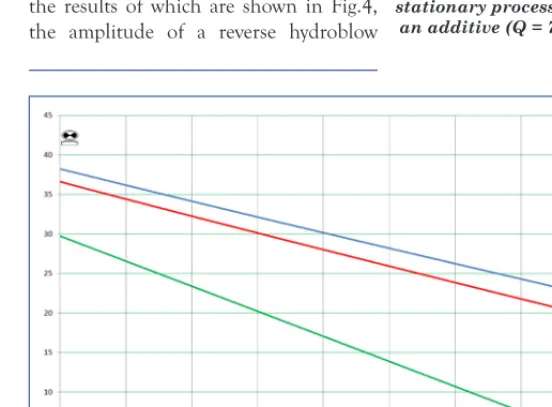
Figure 4 shows the results of pressure calculation at the hydroblow wave front during a simulation of instant valve closing for two variants: the flow of a
liquid without additives, and of a liquid containing DRA in a concentration which guarantees a set efficiency given the following choice of initial data:
Dnominal = 1 m L = 8 x 10⁴ m
Q0 = Q0A
= 1.75 m3/s
r = 860 kg/m3
ν = 10 cSt
y = 0.272327
Valve closure (where there is by-pass through a pump station) was simulated by instant switching of the receiving tank with a set initial fill height to a tank with fill height corresponding to the pressure obtained from Zhukovsky’s formula for instant valve closure. For the calculation, the results of which are shown in Fig.4, the amplitude of a reverse hydroblow
Fig.3. DRA efficiency according to Equn 19:
blue line: calculated DRA efficiency red line: set DRA
efficiency
Fig.4. Pressure at the shock-wave front at an instantly closing valve:
green line: hydro-slope red line: maximum pressures during
non-stationary processes without additive (Q = 6300 m3/hr)
black line: maximum pressures during non-stationary processes with
an additive (Q = 7385 m3/
wave for a liquid containing DRA is 1.6 kgf/cm2 higher than the wave amplitude
of a liquid without additives. The parametric calculations confirm that the intensity of wave processes is higher in a liquid containing DRAs than in a liquid without them. It should be noted that this is relevant not only for a hydroblow wave, but also for depressurizing wave, which can lead to a complete halt in a pump station functioning due to protection activation. This points to the need to adjust algorithms and the hardware components of station-protection systems for pipelines when DRA use is intended. The calculation results obtained for model pipelines will be applied to real ones as well. With real (gradual) valve closure, the amplitude of the generated wave is characterized by a continuous profile, associated with the law of closure and the distance from the controlled cross-sections. This raises the issue of determining the rational law of closure for each mainline block valve to ensure safe pipeline operation.
Conversion formulas for pressure
distribution behind the wave
front
The distribution of liquid parameters between the instantly closing valve and the hydroblow wave front is described by the system in Equns 6 with boundary conditions for characteristics. Symmetrical
schematization [1] of the condition Qr(0, t) = 0 leads to the classical Goursat problem (the characteristic Cauchy problem). In this case, an approximate analytical solution can be obtained more easily than a solution to the Cauchy problem. As the analytical solution of this problem is already obtained from the linear friction law, it is possible to control the degree of approximation (after linearizing the hydraulic resistance function, for example, according to [1]). An approximate analytical solution (Equn 6) can be found in the Equns 22 (below),where
p p p+, ,
0 are pressures, respectively,
at the wave front (defined by Equn 14), at the valve, and the average pressure (between the wave front and the valve)
Qp+ is the mass flow rate at the wave
front (defined by Equn 11).
The time functions p p0, are assumed
to be determined from the integral laws of conservation of mass and of momentum in liquid. Substituting the above relationships in the first two Equns 6, they can be integrated with respect to variable x between 0 and x = ct. Normal algebraic transformations then Equns 23 (below).
Therefore, applying Zhukovsky’s formula means that a simple method can be proposed for on-line calculation of
Q x t x
ctQ t
p x t p x
ct p p p
x
ct p
ρ , ρ
,
( )
=( )
( )
= +(
− −)
+ +
+
+ +
0 0
2
2 3 2 3 pp0−2p
p
p t
p
t p
c
f Q dt t
p p ct
f dQ
dt
t
=
=
+ −
>
= +
+
+ + +
+
+
∫
0
1 0
2
0 0
0
0
ρ
ρ −− + +
−
(
)
+( )
( )
×+ +
+ +
∫
c
f Q f Q
g z z
f ct Q
x
ct
2
8
0 0 02 0 0 0
0 2
0
2
2
ρ ρ
ρ
β ρ
ρ χρ λ Re
ρρf dx
2
(22)
the maximum pressure distribution during transient processes for trunk pipelines, including oil transportation using DRAs. Equations 22 and 23 can be used to determine the pressure at the characteristic points of the curve for pipeline load-bearing capacity. From Equns 14, 22, and 23, it follows that the pressure distribution in a hydroblow wave (formed at time t = 0 in section x = 0), spreading upstream, is written as shown in Equns 24 (below) for turbulent flow in the Blasius regime, where
P(x) is the pressure distribution in the pipeline under hydroblow conditions;
Pst(x) is the stationary pressure distribution along the length of the pipeline, previous to the hydroblow;
∆P(x) is the amplitude distribution
of the hydroblow wave along the length of the pipeline, which is calculated according to formulas (14), (21).
With the known function of distribution Pst(x), relationships (24) allow maximum possible pressures to be evaluated for oil pump stations shut-downs or instant section valve closures in linear pipeline parts, without performing numerical calculations in a system of differential equations in partial derivatives.
Stationary pressure distributions along
the length of the pipeline, preceding the hydroblow, and conversion Equns 20 and 21, make it possible to obtain one of the distributions (a liquid containing or not containing DRA) in hydroblow conditions where only distribution for the other liquid is available. It would therefore be useful to supplement previous relationships with conversion formulas for stationary distributions. Taking into consideration Equn 9, it can be found that conversion formulas for stationary distributions are similar to Equn 2 are as follows:
P x P x
P x P x
stA st Q
st stA
Q
( )
=(
(
−)
)
( )
=−
(
)
Ο
Ο
1
1
ψ
ψ
(25)
Thus, Equn 24 and Equns 20, 21, and 25 make it possible to predict the impact of DRA on the overpressure in a hydroblow wave spreading upstream. The final relationships can be written as given inEquns 16 and 17 (overleaf).
If necessary, a more precise analytical evaluation can be obtained from the control calculation in the initial system of differential equations. The use of such a combined approach reduces the time to solve problems which require calculations involving multiple variants.
According to the relationships above, the
p P x P x
P x
P x
L x ct t L
c
p x
ct p
st
st
+= +
=
− ≤ ≤ − ≤ ≤
+ −
( ) ( )
( )
( ),
,
(
∆
0
2 3
0 22 3 2
0 0
2 3
0
2
0
0
p p x
ct p p p
ct x t L
c
p x
ct
− +
+ −
− ≤ ≤ ≤ ≤
+
+) [ + ]
,
(
pp p p x
ct p p p
L ct x L
c t
L c
− − +
+ −
− + ≤ ≤ ≤ ≤
+ +
2 3 2
0 2
0
2
0
) [ ]
,
conversion method of overpressure in the hydroblow wave comes down to making a transformation which converts one of the solutions for the amplitude of the shock wave into the other (i.e. an equivalence transformation). At the same time, we were limited by the transformation of the spatial independent variable
xO =ζ (| |)x o rxA = (| |)η x , w h i c h
guaranteed identical implementation of the ratios ∆PA(| |)x =∆PO( (| |))ζ x or
∆PO(| |)x =∆PA( (| |))η x .
In general, the pressure-conversion method is formulated as the identification and application of the equivalent transformation, which converts the system of equations describing a liquid without a certain feature (a property), to the system of equations describing a liquid with this feature (and vice versa).
The theory of invariant transformations was developed in Ref.15. An analogue for the transformations necessary for our purposes are equivalent transformations of one-dimensional equations for gas dynamics. Outlining the theory and algorithm for forming equivalent transformations is beyond the scope of this article; it should however be noted that they can be separated explicitly [15]. A similar method of forming flow parameters for a liquid with some particular property, using ‘invariant conversion’ of the flow parameters for the liquid without this property, was successfully used in Ref.16.
Parametric analysis of DRA influence on transient processes allows the following recommendations to be made:
• in order to ensure safe pipeline operation, where DRA use is intended, analysis of the transient processes should be carried out for the liquid with DRA content; • conversion formula Equn 26
and adjustments of protective settings (where necessary) should be applied for pipelines, where transient processes are calculated, without taking into account the possible use of DRAs;
• conversion formula Equn 27 and the subsequent adjustment of protective settings should be applied where DRA usage is rejected;
• the possible need to reduce the allowable operating pressure at the pump-station output should be considered when choosing the DRA concentration to increase the pipeline throughput capacity; • it is advisable to assess the
contribution of transient processes in cyclic loading of the pipe sections by applying the formulas in Equns 14 and 24.
Two-phase flows
Single-phase flows, discussed above, do not exhaust all the possible variants of
P x P x P x
x d c
Q
A
st Q
Q Q
( )
=(
(
−)
)
+( )
= − − + −
(
)
−Ο Ο Ο
Ο
∆
1
64 1
64
3
ψ
π
ψ ψ
Re ln exp QQ
d c x
−
−
π 3 Re
P x P x P x
x d c
Q
st stA
Q
A A
A Q
Ο
( )
= ∆−
(
)
+
( )
=
− −
−
− 1
64
3
ψ
π Re ln ψ exp
664
1
3
Q
d c x
Q
−
−
−
π
ψ
Re
(26)
transported hydrocarbon liquid motion in a real pipeline. For example, there are ‘summit’ points in pipeline routes with hilly or mountainous topographies, which are followed by a downstream flow discontinuities and transitions to two-phase flow with free surfaces (the pipe cross-section will not be completely filled with liquid). Many researchers have devoted their works to solving individual practical problems linked to calculating the flow rate, the filling degree of the pipe cross-section and the length of the gravity-flow section. It has been established that the zone of disturbance for two-phase flow at the inlet of a downhill section is longer (by one order or more) than that for single-phase flow. Under these circumstances, the additive can be expected to have a significant impact on the volume and length of the gravity-flow section, on the dynamics of formation and disappearance of vapour-gas cavities in non-stationary processes, as well as in transition from one pumping mode to another. A section downstream the summit point is not hydraulically connected with the head section (before the summit point), meaning that disturbances with finite amplitude do not spread upstream towards the pumping station. Consequently, the procedure for assessing DRA impact in the head section does not differ from the previously examined scenario and is of no interest in terms of safe pipeline operation.
Conclusions
A new analytical solution was obtained for the pressure at the shockwave front in turbulent flows during pipeline transportation of weakly compressible liquids.
A method of recalculating shock pressure values was proposed for pipeline transportation of liquids where DRAs are used. Corresponding analytical relationships were presented.
The necessity of establishing protective settings was demonstrated using analysis
of non-stationary processes in liquid flows containing DRAs.
References
1. I.A.Charny, Unsteady motion of real liquid in pipes. Gostechteorizdat, (1951) p 223.
2. M.V.Lurie, Book of problems for the pipeline transport of oil, oil products and gas: textbook for universities. Nedra-Businesscenter, (2003) p 349.
3. U.P.Belousov, Drag reducing agents for hydrocarbon liquids, Novosibirsk: Nauka, (1986) p. 144.
4. N.E.Zhukovsky, Hydroblow in water pipes, Gostechizdat, (1949) p. 103.
5. I.P.Ginzburg, Applied fluid and gas dynamics, Leningrad University Publisher, (1958) p. 338.
6. T.I.Lapteva and M.N.Mansurov, Leak detection for non-steady flow in pipes, Oil and Gas Engineering: Electronic Scientific Journal 2 (2006), http://ogbus.ru/ authors/Lapteva/Lapteva_1.pdf (access date: 14.03.2017).
7. E.L.Levchenko, S,B.Nikolaev, and L.M.Bekker, The problem of applying the pipeline surge relief system in oil pipelines of Transneft JSC, Pipeline Transport of Oil 12 (2001) pp 19-27.
8. V.V.Zholobov, D.I.Varibok, and V.U.Moretsky, Simple wave equations describing flow in a weakly compressible hydrocarbon liquid in an elastic cylindrical pipe, Science and Technology of Pipeline Transportation of Oil and Oil Products 2 (2011) pp 44-47.
9. M.I.Valiev, V.V.Zholobov, and S.A.Savinov, Development of a mathematical model and investigation of the shockwave structure in an elastic coaxial pipeline, ibid. 2 (18) (2015) pp 36-40.
10. V .S.Stanev and Sh.I.Rakhmatullin, Considering hydroblow attenuation in a trunk pipeline, Oil Industry 9 (2003) pp 98-99.
11. V.S. Stanev, A.G.Gumerov, K.M.Gumerov, and Sh.I.Rakhmatullin, Strength assessment of trunk pipeline section with hydroblow taken into account, ibid. 4 (2004) pp 112-114.
12. I.O.Zolotov, S.A.Strelnikova, and A.O.Losenkov, One peculiarity of start modes of pipeline operation, ibid. 3 (2011) pp 102-105.
spreading in a turbulent flow of a long pipeline, Acoustic Journal. 55 (2) (2009) pp171-179.
14. M.Y. Kurakina, V.P.Radchenko, and V.A.Yufin, The problem of unsteady motion of a dripping compressible liquid in pipes with different friction laws, Journal of Applied Mechanics and Technical Physics 1 (1976) pp87-94.
Rio Pipeline Conference 24-26 October 2017 Rio de Janeiro, Brazil www.ibp.org.br
Rio Pipeline Conference and Exposition aims at gathering professionals of technical and managerial level in search for knowledge on cutting-edge technologies and the best management practices in the area.
Gas Asia Summit & Exhibition (GAS) 25-27 October 2017
Singapore
www.gasasiasummit.com/
The event aims to address all aspect of the gas and LNG value chain from the upstream to the downstream and power sector as well as highlight new dynamics that are revolutionizing the Asia gas market today.
European Autumn Gas Conference 6-8 November 2017
Milan, Italy www.theeagc.com/
EAGC is Europe’s commercial and strategic gas conference, used by the most senior executives from the world’s largest gas companies to network with peers and customers, review trends, question policy and agree future strategy.
2017 Pipeline Leadership Conference 8-9 November 2017
Dallas, TX, USA plconference.com
The Pipeline Leadership Conference is a new event directed toward top executives involved with building and operating oil and gas pipelines throughout North America. The event will attract thought leaders to discuss innovative approaches and best practices for managing new construction, ensuring safety, improving efficiency and overcoming challenges from inside and outside the industry
Listing of forthcoming industry events
(continued from p 114)
continued on p152
15. L.V.Ovsyannikov, Group analysis of differential equations, Nauka (1978) p.400.