Path Clustering: Grouping in an Efficient Way
Complex Data Distributions
Abstract: This work proposes an algorithm that uses paths based on tile segmentation to build complex clusters. After allocating data items (points) to geometric shapes in tile format, the complexity of our algorithm is related to the number of tiles instead of the number of points. The main novelty is the way our algorithm goes through the grids, saving time and providing good results. It does not demand any configuration parameters from users, making easier to use than other strategies. Besides, the algorithm does not create overlapping clusters, which simplifies the interpretation of results.
Keywords: Cluster, grid, complexity, points, shapes.
R. Q. A. Fernandes1, W. A. Pinheiro1,2,3, G. B. Xexéo3, J. M. de Souza3 1 Centro de Desenvolvimento de Sistemas, SMU, Brasília, DF, CEP, Brazil. 2 Instituto Militar de Engenharia, Praia Vermelha, Urca, Rio de Janeiro, RJ, CEP, Brazil.
3COPPE/UFRJ, Universidade Federal do Rio de Janeiro, RJ, PO Box 68.501, Brazil. E-mail: [email protected], [email protected], [email protected], [email protected] Published Online: 28 December, 2017
The Author(s) 2017. This article is published with open access at www.chitkara.edu.in/publications
Journal on Today’s Ideas – Tomorrow’s Technologies, Vol. 5, No. 2, 2017 pp. 141-155 INTRODUCTION
In spite of the fact that many clustering algorithms have been proposed in the last years [1], it is still a challenge to find irregular shaped clusters from large data sets in acceptable time not demanding too many computational resources. Methods that are able to identify arbitrary shapes impose restrictions of processed data size sets in order to maintain admissible levels of memory usage and processing time.
In the context of Big Data and Data Mining, it is quite relevant the ability of finding clusters without knowing features of the data sets to be clustered. Often, these areas have to deal with large data sets that may produce clusters with arbitrary shapes from different sources, such as: geographic systems, medical systems, and sensors, among others.
This way, clustering algorithms should present some features, such as: ability of assembling clusters of arbitrary shapes and high dimensionality data, capacity of dealing with large data sets having noise and outliers, independence of data order and low time complexity. These characteristics of clustering techniques allow discovering patterns that were not forecast previously. Current clustering algorithms have facing problems to execute these tasks.
Fernandes, R.Q.A. Pinheiro, W.A. Xexéo, G. B.
De Souza, J. M.
This work presents a new clustering algorithm, named Path Clustering, which addresses these features, having better performance than some competitor algorithms existent in literature. Despite the existence of grid clustering algorithms not be something new, the main novelty of Path Clustering is the way it goes through the grids, saving time and getting good results in terms of formed clusters. It considers points allocated in a space divided in small square forms, named tiles (subdivisions of a space in squares, cubes, etc). Neighbors tiles containing one or more points are grouped, which may create a clustering path. This strategy allows building clusters of irregular shapes, independently of data order, and with low complexity. In this context, a relevant cluster in this paper follows the definition related to Contiguous Cluster (Nearest neighbor or Transitive) given at [17]: “A cluster is a set of points such that a point in a cluster is closer (or more similar) to one or more other points in the cluster than to any point not in the cluster”.
The experiments demonstrate our strategy is scalable and provide clusters of good quality when it is compared to other clustering algorithms. At the same time, it allows to find complex patterns from arbitrary data distributions, irregular or not.
The rest of our work is organized as follow: Section 2 presents the related work, Section 3 details the proposed algorithm, Section 4 shows the experiments and Section 5 presents our remarks and points out future works. RELATED WORK
The traditional clustering techniques generally divide clustering algorithms in two main classes: hierarchical and partitioning algorithms [2]. However, in the last years, many different techniques have been proposed trying to reduce the runtime, improve the quality and deal with multidimensional data [3]. These techniques have been applied in many different areas, such as Biomedical Informatics [19].
The hierarchical clustering algorithms make possible to have different visions of grouped objects and it includes agglomerative and divisive methods [4]. The agglomerative methods use a bottom-up strategy. They start with small clusters that are grouped in bigger clusters successively, having algorithms of complexity equal to O(n2) in the best scenario. The divisive methods adopt a top-down strategy,
dividing the clusters progressively. Thus, their complexity is O(2n), which is much
worse than the complexity of agglomerative methods.
Path Clustering: Grouping in an
Efficient Way
Complex Data Distributions K-means aims at minimizing the average squared Euclidean distance of data
from their centers. The centers can initially be chosen randomly and then they are recalculated until either a stop criterion is reached or a number of iterations are executed. K-medoids is similar to K-means, but an object that really exists represents the center of each cluster. The complexity of these algorithms is O(n). But they tend to form Voronoi sets [6], failing to more complex distributions. Another problem of K-means is the necessity of a parameter that inform the number of clusters. Some authors [20] work for providing strategies to discover the number of cluster in a data set, which could reduce the necessity of getting this information from the user.
Density-Based Algorithms [7], such as DBScan, define different clusters based on minimum number of points, radius of a region (r), core points, reachable points and outliers. A core point is a point that can connect directly at least to a minimum number of points within distance r of it. Points that can be connected directly to a core point are called reachable points. All points that are not core points or reachable points are called outliers. Based on this, a cluster is formed by a core point together with all reachable points from it, core or non-core. These methods generally work with numerical attributes and do not produce good results if the clusters have densities too different. Their complexity is O(n log n).
Other strategies of data clustering aim at dividing the data space in segments limited by multi-rectangular shapes. These strategies include Grid algorithms [5]. It deals with geometric shapes to aggregate data sets. Therefore, it stops treating points individually, after allocating them in shapes. This approach produces algorithms with O(n) complexity, where n is the number of points. GRID algorithms may work with attributes of different types and multiple dimensions. Normally, Grid algorithms apply complementary strategies, such as: density, partitioning and hierarchical methodologies, providing better flexibility for different applications. Bang Clustering, STING, DOC, MineClus and INSCY are examples of Hybrid Grid Strategies. Many times these strategies use heuristics to prune points, clusters and/or dimensions, which may become difficult to measure with precision their complexity.
Bang Clustering [8], which is an improvement of GridClust [9], mixes some ideas of hierarchical clustering and density-based algorithms to build grids resolutions through dendograms, having complexity O(n) for several distributions and O(n2) in the worst case [3].
Fernandes, R.Q.A. Pinheiro, W.A. Xexéo, G. B.
De Souza, J. M.
is O(k) in the worst case, since empty cells do not need to be stored in the tree [3]. DOC [11] establishes a subspace cluster using hypercubes of fixed side-length containing a minimum of points. A parameter sets the balance between the dimensionality and the number of elements to be clusterized. It uses a random search algorithm to find the subspace from an initial seed of sampled points. MineCLUS [12] is derived from DOC, however, it uses a deterministic strategy to search the projected cluster based on a sample seed point.
INSCY [13] uses a tree (SCY-tree) to produce high dimensional clusters. It compares each point of the base clusters in order to merge the base clusters having points in common, generating higher dimensional clusters. INSCY has complexity
O(2kn2), where k is the dimensionality of the maximal subspace and n corresponds
to the size of a data set.
Table 1 shows a comparison of some attributes of the clustering methodologies presented previously. One of the problems involves to set the best values of the algorithms parameters, because some of them are not intuitive for regular users and demand some time and experimentation to reach correct values (for each clustering scenario).
Our approach, which is better detailed in the next Section, uses the number of points to build grid resolutions automatically. Therefore, our algorithm does not demand any parameter from users. The concept of neighbor’s tiles forms clusters, which makes the algorithm simple, less complex and faster than other initiatives, keeping a good level of quality for the clusters. The clusters are assembled when the algorithm walks through the tiles. Tiles containing one or more points that have as neighbor another tile containing also one or more points receive the same color. When there is no path (i.e. one or more tiles containing one or more points) that connects tiles containing one or more points, these tiles receive different colors. Thus, as colors are related to clusters, they belong to different clusters.
Table 1: Algorithms Comparison
Algorithms Parameters clusters with arbitrary Ability of building
shapes Data order
Complexity of Algo -rithms (n = number of
points;
k = number of grids)
Hierarchical
Clustering
Points and Minimal Distance among groups
Reasonable.
Some implementa-tions are depen-dent of data order (average linkage) and others are not suitable to deal with noise (Single or complete link-age) (Khan, L. & Luo, F., 2005).
Divisive is O(n2) and Agglomerative is
Path Clustering: Grouping in an
Efficient Way
Complex Data Distributions Algorithms Parameters clusters with arbitrary Ability of building
shapes Data order
Complexity of Algo -rithms (n = number of
points;
k = number of grids)
K-means
and K-me
-doids
Points and Number of clusters.
Limited. They tend to form Voronoi sets and they fail for distributions that are more complex.
They depend of data order. They are sensitive to initialization. O(n). Densi-ty-Based Algorithms Points, Radius r and Minimum Num-ber of Points.
Reasonable. They do not produce good results if the clus-ters have densities too different.
They do not depend of data order.
DBScan (n log n
using an accelerating index structure and for
non-degenerated data and O(n2) in the worst
case).
GRID
Hybrid
Algorithms
Vary according to the imple-mentation.
Very good. The
challenge is to find the
correct resolution (grid size) for different distri-butions.
Generally, they do not depend of data order.
Bang Clustering is
O(n2) and STING is O(n) for building the tree and
O(k) for clustering. DOC and MineClus use heuristic (authors
do not discuss algo-rithm complexity). INSCY is O(2kn2). Path
Clus-tering Points. Reasonable. It does not depend of data order. O(t)number of tiles., where t is the In this work, the following algorithms are compared to Path Clustering: K-means, DBScan, INSCY, DOC and MineClus. Some of these algorithms can optionally generate overlapping or non-overlapping clusters. In this work, we set all algorithms in order to not produce overlapping clusters.
PROPOSED APPROACH
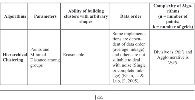
To illustrate our strategy, we generate a data set represented by points in a space. Fig. 1 shows these points (graph A) and also presents some results (graphs B, C and D) obtained using some basic ideas of Path Clustering algorithm for three different resolutions (different number of tiles).
The first resolution divides the space in one hundred (ten x ten) tiles. If a tile contains one or more points, it receives a color. A tile containing one or more points that has a contact with other tile also containing one or more points receive the same color. Tiles containing one or more points separated by tiles containing no points receive different colors. This strategy builds the clusters showed in Fig. 1 (graph B).
Fernandes, R.Q.A. Pinheiro, W.A. Xexéo, G. B.
De Souza, J. M.
Comparing the results obtained by these resolutions, it is possible to observe that the latter provides clusters that are closer to the expected from the original data distribution.
However, if we continue dividing the space in more tiles (1000 x 1000 tiles), as presented in Fig. 1 (graph D), they become too small. In this case, some tiles do not touch each other as they should (tiles distance is smaller than points distance), which produce more clusters than expected. Thus, the analysis of the proposed strategy demonstrates the relevance of choosing the correct number of tiles to obtain good results.
For the sake of simplification, in this paper, we consider that all points are contained in a space of two dimension (axis x and y) with a square format.
Figure 1: Path Clustering Algorithm for three different resolutions To reach good results, it was defined that the maximum resolution, that can vary according to the number of points, should generate a complexity lower or equal to O(n). Besides, if necessary, the transition among resolutions should be done easily. For example, four tiles in a flat space could be transformed in one big tile for the next resolution. In this case, the tiles of previous resolutions are equivalent to points for the next (lower) resolution. Thus, resolution was defined as a power of two, in order to make easier generating clusters for other resolutions through reuse of previous results (merging smaller tiles). Therefore, the results of higher resolutions can be used to generate results for lower resolutions.
In this context, this work defines Resolution Scale (RS) as:
RS = 2 x (1)
Where:
x = upper limit of [log2((number of points)(1/number of dimensions))] (2)
For instance, if the number of points is 100 and the number of dimensions is 2, then RS is equal to 16. If the space size that contains the points is equal to 20cm x 20cm, then the tile-side size is 20/16=1.25 and the total number of tiles is 16x16 (total of 256 tiles).
Path Clustering: Grouping in an
Efficient Way
Complex Data Distributions 1. It finds the maximum number of tiles considering only the number of points;
2. It paints tiles without considering density of points;
3. It uses a greedy strategy, just looking for local neighbors. Thus, it depends on the tiles size;
4. It has the complexity that is given by the maximum number of tiles (maxi-mum RS) that is O(n).
5. It is independent of data order; and
6. It has the capacity of finding clusters with arbitrary shapes in an efficient way.
Considering this, the pseudocode of the algorithm is presented as follows (← means ‘to receive’ and = = means ‘is equal to’):
Algorithm PathClustering Input: P points
Output: T[resolution] list of colored tiles
1. num-of-points ← points from P
2. S ← calculate the minimum space in a square format necessary to
contain all points from P
3. number of dimensions← 2 (for a flat space)
4. X← superior limit of [log2((num-of-points)(1/(number of dimensions)))])
5. RS ← 2 x
6. N←(RS)2 (approximately equal to num of points )
7. Tiles[] ← Create N tiles in S, dividing S in RS x RS=N tiles
8. Groups[] ← Create N groups in S (Each group can contain one color
and one or more tiles)
9. Colors[] ← Create N colors
10. While t = Tiles.next (from left to right, top to bottom):
10.1. if t contains some point p from P in S then t.point=true else
t.point=false 11. While t = Tiles.next:
11.1. group ← Groups.next
11.2. color ← Colors.next
11.3. if t.point==false then continue
11.4. if t.point==true and t.group is null then
11.4.1. {t.group ← group; group.color ← color; group.tiles ← t}
11.5. if t.group is not null then
11.5.1. {group ← t.group}
11.6. NE ← find neighbors of t in Tiles (Up to 8 neighbors)
11.7. While ne = NE.next: (Check neighbors’ groups)
11.7.1. if ne.group is not null and ne.group!=t.group then
11.7.1.1. {add ne.group to t.group (generates a bigger t.group
Fernandes, R.Q.A. Pinheiro, W.A. Xexéo, G. B.
De Souza, J. M.
11.7.2. if ne.point==true and ne.group is null then
11.7.2.1. {ne.group ← group; group.tiles ← ne}
EXPERIMENTS
To compare the results obtained and execution time of Path Clustering with other algorithms of equivalent complexity, we carried out a set of experiments. We selected the following algorithms: K-means, DBScan, INSCY, DOC and MineClus (one or more representative of each category showed in Table 1, except by hierarchical clustering). The hardware used in the experiments was an Intel Core i3 3.6GHz processor with 4GB RAM and the software used was Ubuntu 14.04.4 LTS. We used implementations of the algorithms kindly shared on web. The implementation of K-means and DBScan were obtained in python [15]. For INSCY, DOC Clustering and MineClus we used the executable software in java from [16].
To compare the algorithms, we built two classes of distributions: Gaussian distributions and Radial distributions. These distributions took as base five random points in a flat space. Therefore, the maximum of five relevant clusters could be obtained. Doing this, we tried to compare the algorithms in different scenarios using just two dimensions. A future work will compare our strategy in a scenario of high-dimensional data. The distributions considered distributions of 100 up to 10000 points. A number of points higher than 10000 was not run because some algorithms caused a high memory consumption avoiding completing these experiments in an acceptable time.
For repeatability, the algorithms configurations used in the experiments are presented in Table 2. For Grid-based algorithms, when possible, we set similar conditions when it was possible.
Table 2: Algorithms Parameters Algorithm Parameters
K-means number of clusters = 5 DBScan eps=0.1, min_samples=10
INSCY Density=1.0, epsilon=1.0, gridSize= number of points, maximalClusterRate=0.0, min-Points=1.0, minSize=1, usingKernel=1
DOC alpha*number of points = 1, beta=0.1 , maxiter=1024, k=5, w=1.0
MineClus alpha*number of points = 1, beta=0.1 , maxiter=1024, k=5, w=1.0, numBins = 1
Path Clustering: Grouping in an
Efficient Way
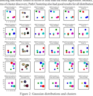
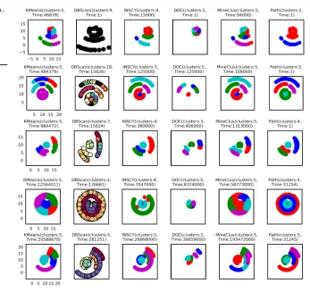
Complex Data Distributions Fig. 3 shows a matrix of graphs containing Radial distributions. The graphs
obey the same pattern used in Fig. 2.
[18] considers that human vision is efficient to find cluster in two dimensions. Therefore, in this paper, relevant clusters are identified visually. In the case of Gaussian distributions, it was obtained the following number of clusters: four clusters for the distribution of 100 points, four clusters for the distribution of 500 points, five clusters for the distribution of 1000 points, five clusters for the distribution of 5000 points and four cluster for the distribution of 10000 points. In the case of Radial distributions, it was obtained the following number of clusters: four clusters for the distribution of 100 points, five clusters for the distribution of 500 points, five clusters for the distribution of 1000 points, five clusters for the distribution of 5000 points and four cluster for the distribution of 10000 points. These values can be verified observing the graphics of Fig. 2 and Fig. 3.
Visually, it possible to observe for Gaussian and Radial distributions that Path Clustering had better results in terms of time than the other algorithms. Besides, in terms of cluster discovery, Path Clustering also had good results for all distributions.
Fernandes, R.Q.A. Pinheiro, W.A. Xexéo, G. B.
De Souza, J. M.
Figure 3: Radial distributions and clusters
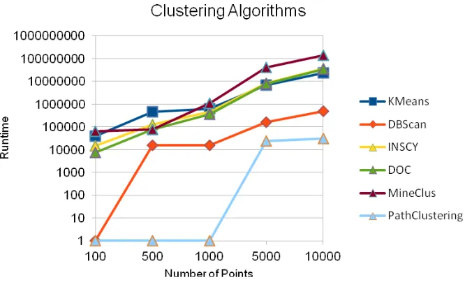
Table 3 and Table 4 reveal the execution time (in microseconds) of the six algorithms for Gaussian and Radial distributions, considering 100, 500, 1000, 5000 and 10000 points. An average runtime is resulted of five executions of an algorithm.
Table 3: Average Runtime for Gaussian Distributions Number
Path Clustering: Grouping in an
Efficient Way
Complex Data Distributions Table 4: Average Runtime for Radial Distributions
Number
of Points Kmeans DBScan INSCY DOC MineClus PathClus-tering 100 46878 <1 15000 <1 94000 <1 500 484379 15626 125000 125000 109000 <1 1000 984472 15624 360000 406000 1313000 <1 5000 12564011 126661 7047000 8324000 58773000 31254 10000 20588678 281251 26868000 36659000 193472000 31245 Fig. 4 shows the total average time comparison (in microseconds) for Gaussian and Radial distributions, considering the values of Table 3 and Table 4. Axis Y is in logarithm scale. The results showed that, considering these two distributions, Path Clustering was more than 10 times faster on average than the second faster algorithm: DBScan.
Figure 4: Total Average Runtime
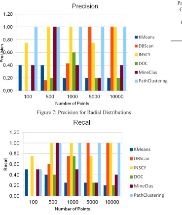
Additionally, to measure the quality of the results, we used two metrics: precision and recall, derived from the Information Retrieval area.
Fernandes, R.Q.A. Pinheiro, W.A. Xexéo, G. B.
De Souza, J. M.
Recall can be defined as the number of relevant returned results divided by the number of relevant results [14]. We used this as the number of relevant returned clusters divided by the number of relevant clusters. In our experiments, the maximum number of relevant clusters was five.
Fig. 5 presents the precision results for Gaussian distributions. Fig. 6 shows the recall results for Gaussian distributions. In three of five tests, Path Clustering got the best results for precision and recall.
Figure 5: Precision for Gaussian Distributions
Figure 6: Recall for Gaussian Distributions
Fig. 7 presents the precision results for Radial distributions. It is possible to notice that Path Clustering got the best possible results in all cases.
Path Clustering: Grouping in an
Efficient Way
Complex Data Distributions
Figure 7: Precision for Radial Distributions
Figure 8: Recall for Radial Distributions
Fernandes, R.Q.A. Pinheiro, W.A. Xexéo, G. B.
De Souza, J. M.
to develop a strategy to calculate the best number of grids according to the distribution and number of points.
CONCLUSION
This paper presents a grouping algorithm named Path Clustering. It is a clustering grid algorithm that divides data space in segments limited by square shapes called tiles. The way used to navigate from one tile to another provides a new faster strategy to group data. It uses a greedy strategy, navigating through local neighbors following a specific path. Tiles containing one or more points separated by tiles containing no points receive different colors. Different colors indicate different groups.
After allocating data items (points) in geometric shapes in tile format, the complexity of our algorithm is related to the number of tiles instead of the number of points. Thus, the number of tiles is fundamental to reduce the complexity of our algorithm. In our strategy, a tile is represented by a square shape and the square-side size is a number related to a concept named Resolution Scale. In order to keep a balance between low complexity and good results for different data distributions, we proposed that maximum Resolution Scale should provide a complexity of O(n), reducing space in memory and time of processing when compared to other algorithms.
Other interesting characteristic is that the algorithm presented in this paper does not require parameters from users beyond the data set itself, making easier to use than many other algorithms.
It was performed a comparative experiment considering Path Clustering and other five algorithms. The experiments demonstrated our strategy is scalable using two type of distributions (Gaussian and Radial) with different number of points. Path clustering showed the best performance in terms of time. Besides, their clusters get a good precision and recall in most part of tested distributions, considering the idea of a Contiguous Cluster (Nearest neighbor or Transitive). At the same time, it allows to find complex patterns from arbitrary data distributions, irregular or not.
Path Clustering implementation used in this work did not apply concurrent computing to execute the processes. Concurrent algorithms can execute processes in parallel, reducing processing time. Thus, we intend to implement this feature in future works, allowing to reduce even more the execution time for grouping data. Besides, we intend to compare the algorithm in a high-dimensional data scenario and calculate automatically the best number of grids according to the distribution and number of points.
REFERENCES
Path Clustering: Grouping in an
Efficient Way
Complex Data Distributions eswa.2014.01.028.
2. Khan, Latifur; Luo, Feng. (2005). Hierarchical clustering for complex data, in press. Int. J. Artif. Intelligence Tools. Vol. 14 No. 5. World Scientific.
3. Aggarwal, Charu C. and Reddy, Chandan K. (2014). Data Clustering: Algorithms and Ap-plications. Chapman and Hall/CRC. ISBN-13: 978-1466558212.
4. Sasirekha, K., Baby, P. (2013). Agglomerative Hierarchical Clustering Algorithm- A Re-view. International Journal of Scientific and Research Publications, Volume 3, Issue 3. ISSN 2250-3153.
5. Berkhin, Pavel (2002). Survey of clustering data mining techniques. Technical report, Ac-crue Software, San Jose, CA, 2002.
6. Telgarsky, M., & Vattani, A. (2010). Hartigan’s method: k-means clustering without vo-ronoi. In International Conference on Artificial Intelligence and Statistics (pp. 820-827). 7. Ester, M., Kriegel, H., Sander, J. and Xu, X. (1996). A density-based algorithm for
dis-covering clusters in large spatial databases with noise. Proc. 2nd Int. Conf. Knowledge Discovery and Data Mining (KDD’,96), pp.226 -231.
8. Schikuta, E., Erhart, M. (1997). The BANG-clustering system: grid-based data analysis. In Proceeding of Advances in Intelligent Data Analysis, Reasoning about Data, 2nd Interna-tional Symposium, 513-524, London, UK.
9. Schikuta, E. (1996). Grid-clustering: a fast hierarchical clustering method for very large data sets. In Proceedings 13th International Conference on Pattern Recognition, 2, 101- 105.
10. Wang, W., Yang, J., and Muntz, R. (1997). STING: a statistical information grid approach to spatial data mining. In Proceedings of the 23rd Conference on VLDB, 186- 195, Athens, Greece.
11. Procopiuc, C.M., Jones, M., Agarwal, P.K., Murali, T.M. (2002). A Monte Carlo algorithm for fast projective clustering Proceedings of the 2002 ACM SIGMOD international confer-ence on Management of data, ACM New York, pp. 418-427.
12. Yiu, M. L. and Mamoulis. (2003). N. Frequent-pattern based iterative projected clustering. In Proceedings of the 3rd IEEE International Conference on Data Mining (ICDM), Mel-bourne, FL, pages 689–692.
13. Assent, I., Krieger, R., Muller, E., and Seidl, T. (2008). InSCY: Indexing subspace clusters with in process-removal of redundancy. In Eighth IEEE International Conference on Data Mining, 2008. ICDM’08, pages 719–724. IEEE.
14. Baeza-Yates, R., Ribeiro-Neto, B. (2011). Modern Information Retrieval: The Concepts and Technology Behind Search. 2011. ISBN-13: 978-0321416919.
15. Scikit. (2017). scikit-learn user guide. Release 0.19.1. Extracted from: http://scikit-learn. org/stable/_downloads/scikit-learn-docs.pdf. 2017.
16. Müller. E., Günnemann. S., Assent. I., Seidl. T. (2009). Evaluating Clustering in Subspace Projections of High Dimensional Data. Home-page: http://dme.rwth-aachen.de/OpenSub-space/. In Proc. 35th International Conference on Very Large Data Bases (VLDB), Lyon, France.
17. Tan, P., Steinbach, M., Karpatne, A. and Kumar, V. (2013). Introduction to Data Mining, (Second Edition). Ed. Pearson. 2013. ISBN-13: 978-0133128901.
18. Jain, A. K. (2010). Data clustering: 50 years beyond K-means. Pattern Recognition Let-ters, Volume 31, Issue 8. 2010. ISSN 0167-8655.
19. Ultsch, A., Lötsch, J. (2017). Machine-learned cluster identification in high-dimensional data. Journal of biomedical informatics, ISSN: 1532-0480.