A bi-level programming approach to coordinating pricing and ordering decisions in a multi-channel supply chain

Journal of Industrial Engineering and Management Studies Vol. 5, No. 2, 2018, pp. 13-37

DOI: 10.22116/JIEMS.2018.80682

www.jiems.icms.ac.ir

A bi-level programming approach to coordinating pricing and ordering

decisions in a multi-channel supply chain

Reza Pakdel Mehrbani1, Abbas Seifi1,* Abstract

This paper investigates the Stackelberg equilibrium for pricing and ordering decisions in a multi-channel supply chain. We study a situation where a manufacturer is going to open a direct online channel in addition to n existing traditional retail channels. It is assumed that the manufacturer is the leader and the retailers are the followers. The situation has a hierarchical nature and is formulated as a bi-level programming problem. The upper level problem is a mathematical model dealing with decisions of the manufacturer, while the lower level is a Nash equilibrium model determining the retail prices and order quantities by formulating the competition between the physical retailers. We consider a price-sensitive linear demand model with an additive uncertain part and analyze the optimal decisions for each sales channel. To enable supply chain coordination, we propose a particular revenue-sharing contract. This contract enables the retailers to set pricing and ordering policies that are equivalent to those in an integrated supply chain. Finally, we examine the impact of the model parameters on the equilibrium with a comprehensive numerical study.

Keywords: Multi-channel supply chain; Pricing strategy; Supply chain coordination; Stackelberg game.

Received: April 2018-18 Revised: June 2018-22 Accepted: November 2018-04

1. Introduction

Today, in order to increase their sales, many manufacturers tend to sell their products through a direct online channel, which enables them to communicate directly with their final consumers. Furthermore, they can track the market trend and changes in the customers' behavior. Although a new online channel raises conflict because of competition between different channels, despite this risk, hybrid distribution is the dominant marketing design (Moriarty and Moran, 1990). A new online store acts like a competitor of existing traditional retail channels, and in fact network conflict is the result of the different roles of the manufacturer as both a supplier and as a retailer (Tsay aAgrawal, 2004).

* Corresponding author; [email protected]

To reduce this conflict, it is important to study the reactions of all players in the supply chain after a direct online channel is added. The pricing strategy of the manufacturer is the main influential factor on the pricing and ordering decisions of retailers, which in turn affect the total network sales. Coordinating pricing and ordering decisions in a multi-channel supply chain is the focus of this paper. Three streams of research can be distinguished about multi-channel supply chains:

A number of studies have discussed the competition between channel players.

Another group analyze the performance of the physical retailers and the manufacturer in presence of an online store. These studies try to determine whether or not a manufacturer should open a direct online channel.

Others have focused on coordination mechanisms with existence of a manufacturer-owned online store in a supply chain.

Cattani et al. (2006) discuss equal pricing scenarios for wholesale price or retail price in a manufacturer-Stackelberg dual channel supply chain. They reach a conclusion that both retailers and customers would benefit from maximizing the manufacturer's profit with equal pricing. Mukhopadhyay et al. (2008) investigate pricing decisions in a mixed-channel model in which the retailer is allowed to add further value to the product before selling to the final customer. Chen et al. (2008) investigate a dual channel considering consumer channel choice model in which the demand faced in each channel depends on the service levels of both channels and determine when the manufacturer should establish a direct channel. Zhang et al. (2012) investigate the effect of product substitutability and pricing strategies under three different power structures (which are manufacturer Stackelberg, Retailer Stackelberg and Vertical Nash) of a dual exclusive channel system where each manufacturer distributes its goods through a single exclusive retailer.

Tsay and Agrawal (2004) show that adding a direct channel may be beneficial for both the retailer and the manufacturer. They show that this is the result of counteracting double marginalization. They stated that paying the reseller a commission for diverting customers toward the direct channel could coordinate the supply chain. There is a same conclusion in Cai (2010). He introduces the channel-adding Pareto zone in which both the supplier and the retailer benefit from adding a new direct channel. He then investigates channel coordination and shows that in the contract-implementing Pareto zone, both the supplier and the retailer gain more profit. Dumrongsiri et al. (2008) show that when the retailer’s marginal cost is high and the wholesale price and demand variability is low, the manufacturer benefits more from the dual channel than the single channel. They also investigate the coordinated supply chain and show that in a centralized system, the overall profit is increased.

Panda et al. (2015) consider a sale network for high-tech product and obtains pricing and replenishment policies under continuous unit cost decrease and concludes that product compatibility to online sales has a significant impact on the pricing policy. Li et al. (2014) consider a dual channel with a risk-neutral manufacturer and a risk-averse retailer and investigates the equilibrium results and shows that the retail price will decrease as the retailer becomes more risk averse.

Contrary to previous studies that consider the problem with just one retailer, this paper investigates the addition of a manufacturer’s online store to n competing retail channels and aims to coordinate pricing and ordering decisions among all players in the network. We consider the problem of supply chain coordination for a multi-channel supply chain in the presence of price competition among all channels. To the best of our knowledge, none of the mentioned articles have discussed the influence of market share on pricing strategies in a supply chain with n competing retailers.

The demand is considered to change according to a linear function of price with an additional random variable. The problem is formulated as a Stackelberg game in which the manufacturer is the leader and the retailers are followers. The resulting mathematical model becomes a bi-level programming problem that is solved using Karush-Kuhn-Tucker conditions for the retailers pricing problem. We find the Stackelberg equilibrium for the wholesale and retail prices in a single-period setting. We also carry out a sensitivity analysis of model parameters and investigate their effects on both wholesale and retail prices. In addition, we consider the cost of lost sales for the whole network and apply a revenue-sharing contract in order to increase total sales in the network. The contract complete the mathematical formulation of the problem and leads to the highest level of coordination, which is similar to a centralized supply chain.

2. Mathematical modelling

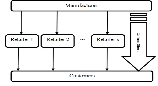
In this section, we introduce the notation and formulation used in our multi-channel supply chain problem. As shown in Figure 1, we consider a single manufacturer that exclusively supplies a single product to n competing retailers. In addition, the manufacturer sells through physical retail channels and a newly added online store (channel 0). These n1 firms compete on price and form an oligopoly. In the whole paper, the subscript 0 represents for the newly opened online store and we use the subscript i (i 1,...,n) to denote physical retailers. Superscripts I , RSC shows the integrated supply chain, supply chain under revenue sharing contract, respectively.

The proposed model in this paper is based on the following assumptions:

Before a selling season, the manufacturer sets the wholesale price w_i for each channel i 1,...,

i n

  , the online store price p ₀ and the production quantity q₀ to be sold through the online channel. It is assumed that the online channel buys the product that is priced at production cost.

Each retailer then sets its own retail price p_i and decides how much to order from the manufacturer (q_i) based on its local demand, which is assumed a random variable.

The manufacturer will then produce the total number of ordered quantities with a unit production cost of c .

There is a shortage cost (s_i  i 0,1,...,n) for each unit of unsatisfied demand in each channel. Excess inventory of channels are salvaged with the value of v_i ( i 0,1,...,n).

In the next subsection, we obtain demand function of all channels and next we model the problem.

2.1. Demand function modelling

To model demand functions of a multi-channel supply chain, a sales network consisting of a direct online channel andnphysical retailers, we need to segment the base market to two different types of online and traditional customers to this aim, we use the concept of “customer acceptance level of the product on online channel”. Different products have different acceptance level on the e-markets. A product with higher acceptance level of online channel will have a higher likelihood of being successful when marketing on the web. An empirical study on the acceptance level of online channel is investigated by Liang and Huang (1998). The study by Kacen, Hess and Chiang (2013) is also a recent survey which provides insights in customer acceptance of web based purchases.

Using the concept of “customer acceptance level“ and adopting a downward sloping linear demand model with an uncertain additive part, that is used widely in the literature (Bernstein and Federgruen, 2004; F. Y. Chen, Yan, and Yao, 2004; J. Chen, Zhang, and Sun, 2012; Yan

et al., 2011), we derive the demand function of the online store (d₀) and physical retailers (d_i  i 1,...,n) as follow:





0 0 0 0

1

0,

1 1,...,

n j j

n

i i i i j i

j j i

d a p p

d a k p p i n

 





 







 

 _{   }

  

       

 





(1)

a



represents the number of customers preferring the online store and



1a



 denotes the number of customers preferring physical stores where

a



[0,1]

. The base market share of each physical retailer is k_i(in a way that

1 1

n i i

k







). As a result the base demand of physical retailer i is



1a k



_i. For more simplification let



_i  



1 a k



_i



. The value of the parameter a

i

p ( i 1,...,n) and p₀ denote the price of physical retailer i and the online store, respectively.



_i ( i 1,...,n) and



₀ thus represent own-price sensitivities of the physical retailer i and the online store. The parameter





0

represents cross-price sensitivity among firms. _i( i 0,1,...,n) is the uncertain component of channel i s' demand function. Probability distribution function (PDF), cumulative distribution function (CDF), and the expected value of this variable are assumed known and are denoted by f_i

 

. , F_i

 

. and _i . It is assumed that the range of _iis



a b_i, _i



. We define the failure rate of random variable _i by

 

.

 

.

_{ }

1 .

i i

i

f r

F



 . The random variable i is said to have the increasing failure rate (that is, IFR)

property if r xi

 

is weakly increasing in x .

Let _{0 0 0}

1 ( )

n j j

p a p p



 





  



and





0, ( ) 1

n

i i i i j

j j i

p a k p p



 



 

   



 i 1,...,n. Thus,

the demand functions of the sales channels are rewritten in the following way: 0 0( ) 0

( ) 1,...,

i i i

d p

d p i n









 



    

 (2)

In the first part of the proposed mathematical model, a decentralized supply chain is considered in which players optimize their own profits instead of maximizing the entire supply chain profit. In the second part, we consider an integrated supply chain and obtain the maximum attainable profit.

2.2. Decentralized multiple-channel supply chain

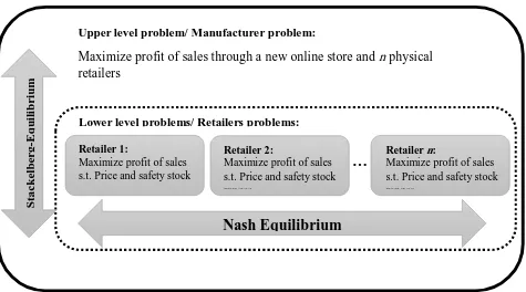
As previously mentioned, in a decentralized supply chain each player pursuits only his interest. We consider the manufacturer a leader who sets the wholesale prices, the selling price in the online store and the amount of safety stock that online store holds. The retailers are followers in this Stackelberg game, and they react rationally to the manufacturer's price in choosing their selling prices and the quantities they order. Because of the hierarchical nature of such a decision making process, we formulate the problem as a bi-level programming problem. In the developed bi-level model, the upper level problem is a mathematical model dealing with decisions of the manufacturer, while the lower level is a Nash equilibrium model determining the retail prices and order quantities by formulating the competition between the physical retailers. This model is different from traditional bi-level programming models because in the lower level we have a Nash equilibrium instead of a typical mathematical model.

The profit function of each physical retailer is modeled as a newsvendor problem with price and order quantity as decision variables and is written as follow:



,



min



,



_i









1, ,

i p qi i pi q di i v qi di s di i qi qiwi i n

 

         

(3) where (.) + _{is defined as the maximum of zero and the quantity in brackets.}

It is clear that _i



p q_i, _i



is similar to a newsvendor model with price and order quantity as decision variables. We use the simplifying assumption in Petruzzi and Dada (1999) and define

i

z with the range



a b_i, _i



as the amount of safety stock that is held at location i and write

i i i

q 



z . With this reformulation, the decision variables for each retailer are p_i and z_i. Thus, the expected profit function of retaileri is rewritten as follows:







 





   

  

E[_i(p z_i, _i)] p_i w_i

 

_i  _i p  p_i  s_i w_i _i z_i  w_i v_i _i z_i (4) In the above-mentioned profit function, _i(z )_i and _i(z )_i are expected excess inventory and shortage, which are obtained as follows:

 

 





 

 





( ) ( ) ( )

( ) ( ) ( )

i

i

i

z

i i i i i i i i i i i

a

i i i i i i i i i i i

z E q d E p z p F d

z E d q E p p z z z

    

   

 

 

       

          



(5)

For more details of _i(z )_i and _i(z )_i please see Appendix A.

The expected profit of the manufacturer E__M



w_i,p z₀, ₀



_ includes the profit he or she obtains from selling the product to retailers and the profit of direct sales through online store:

S

ta

c

k

el

b

er

g

-E

q

u

il

ib

ri

u

m

Lower level problems/ Retailers problems:

Nash Equilibrium

Retailer 1:

Maximize profit of sales s.t. Price and safety stock ranges

…

Retailer 2:

Maximize profit of sales s.t. Price and safety stock ranges

Retailer n:

Maximize profit of sales s.t. Price and safety stock ranges

Upper level problem/ Manufacturer problem:

Maximize profit of sales through a new online store and n physical retailers

s.t. Constraints related to safety stock and prices ranges







 





 





 











0 0 0 0 0

1 1

0 0 0 0 0 0 0

E , , +

( ) ( )

n n

M i i i i i i

i i

w p z c p z w z p p p

p s c z c v z

   

 

 

      

  _{ }

  _{ }

      





(6)

Now the hierarchical decision-making process of the problem is formulated as following bi-level programming problem:

Upper-level Problem/Manufacturer problem:







 





 



 













0 0

0 0 w ,p ,z

1 1

0 0 0 0 0 0 0 0 0 0

Max E , ,

+ ( ) ( )

i

n n

M i i i i i i

i i

w p z c p z w z p

p p p s c z c v z

 

 

 

 

     

  _{ }

  _{ }

       





0

0

0 0 0 . .

w 1, 2,..., 1, 2,...,

i

i

s t

c i n

p w i n

p c

a z b

  

  

  

(7)

Lower-level Problems:

Physical retailer 1:



 





 











1 1

1 1 1 1 1 1 1 1 1 1 1 1 1 1 1 1

,

1 1 1

Max E , ( ) ( )

s.t.

p z p z p z v z

a z b

p w   p s w w

         

 

 

 



(8)

Physical retailer 2:



 





 











2 2

2 2 2 2 2 2 2 2 2 2 2 2 2 2 2 2

,

2 2 2

Max E , ( ) ( )

. .

p z p z p z v z

s t

p w p s w w

a z b

 

         

 

 

 



(9)

⁞

Physical retailer n:



 





 











,

Max E , (z ) (z )

s.t. n n

n n n n n n n n n n n n n n n n

p z

n n n

p p w p p s w

z b

w

z v

a

 

         

 

 

 



(10)

In the upper-level problem, the manufacturer sets wholesale prices (w_i), the price (p₀) and

online store rather than through the manufacturer. We need the range a₀ z₀ b₀ to conquer the randomness of the demand function. The lower-level problems consist of n competing retailers who play a simultaneous move game with sale price (p_i) and safety stock (z_i) as decision variables. To tackle the problem, we should find the Nash equilibrium of the lower-level game and then the Stackelberg equilibrium of the model. The solution method is discussed in the next section.

3. Solution method of decentralized multi-channel supply chain

A common approach to solve a bi-level problem is to replace the lower-level problem with its Karush-Kuhn-Tucker conditions and convert the bi-level problem to a single-level optimization problem. This procedure is not directly applicable to our bi-level model, because in the lower level we have ncompeting retailers rather than a single retailer. To find the optimal solution of model (8)-(11), we need to obtain the Nash-equilibrium of retailers’ game in the lower level problems. By having the Nash equilibrium and putting it into the upper level model, we can convert the bi-level problem to a single level mathematical programming problem.

3.1. Nash-equilibrium of the lower level players

A set of paired retail prices and safety stocks,





p z₁*, ₁*

 

, p z₂*, ₂*

 

,..., p z_n*, _n*





, is a Nash equilibrium of the lower level system if each retailer’s price (pi ) and safety stock (zi) is a

best response, i.e., for all i , p_i and z_i: E__i



p z_i*, _i*,p_*_i,z_*_i



_E__i



p z_i, _i,p_*_i,z*_i



_ 1,...,

i n

  where i shows the competitors of channel i . To find the Nash equilibrium, as stated by Cachon (2003), it is enough to solve a system of best responses of game players. Theorem 1.Assume the random component of each retailer’s demand has an IFR distribution, then E[_i(p z_i, _i)]is jointly quasiconcave in p_i and z_i, so a pure-strategy Nash equilibrium exists.

Proof. Please see Appendix B.

Lemma 1. If retailer i’s safety stock is considered fixed, the optimal price of this retailer is a

unique function of the decision variable zias follow:

0

* ( ) ( )

( ) =

2 2 2

n

i i i j i

j

j i i i i i i

i i i r

i i i

w p

z z

p p z p

   

  

 

  

 

   



(11)

in which

0

2

n

i i i j i

j j i i

r

i

w p

p

   

  

  





Proof. Please see Appendix B.

Substituting *

( )

i i i

p p z into the retailer i’s profit function, the optimization problem of each



 





 











0

Max E ( ), ( ) ( ) ( ) ( )

s.t.

( ) ( )

2 2

i

i i i i i i i i i i i i i i i i i i i

z

i i i

n

i i i j i

j

j i i i

i i

i i

p z z p z p p z z v z

a z b

w p

z p z

w   s w w

                                ) 12 (

The new profit function, with the single variable z_i, is called reduced profit function.

The optimal stocking and pricing policy for the retailer i in the multiple channel supply chain is to stock q_i* (p_i*)z_i*, where p_i* is specified by Lemma 2 and z_i* is determined according to the following lemma.

Lemma 2. If 1)

0

( 2 ) 0

n i j j j i i

i i i

w s

p  a

 

 

 





  and 2)F_i(.) is a distribution function

satisfying the condition 2



( )



2 i( i) 0

i i

i

dr z r z

dz

  for a_i z_i b_i , where (.) (.)

1 (.) i i i f r F 

 is

the failure rate, then *

i

z is the unique z_i in the region [ ,a b_{i i}] that satisfies





E ( ),

0

i i i i

i

d p z z

dz



 

 _{ }

Proof. See the proof of Theorem 1 in Petruzzi and Dada (1999).

Using Lemmas 1 and 2, there is only one unique value of the first derivative of reduced profit function over decision variable z_i. As a result the best response of retailer i is the unique solution of (13)–(14):





_

_

_

_{ }

_

dE ( ),

0 _{i i} ( ) _i 1 0

i i i i

i i i

i

i i

p z z

p z

dz w  v  s v F z



 

 _{     (13)}

0

( ) ( )

2 2

n

i i i j i

j

j i i i

i i i i w p z p z













       



(14) As a result, the Nash equilibrium of n competing retailers, which is the solution of the lower level problem, is given by the following system:







 



0

1 =0 1, 2,..

( )

( ) ( ) =

.,

1, 2,.

2 2 . ,.

i i n

i i i j i

j

j i i i

i i

i i

i i i i i i

w p z

w

v s v F

p

z z

z i n

i n p

 









               

To convert the problem (8)-(11) to a single-level optimization problem and obtain the Stackelberg equilibrium, the system (15) is put into the upper level model. The resulting model (16) is a typical mathematical programming problem and its solution can be obtained using GAMS.

Single-level model:

























0 0

0 0 0 0 0

w ,p ,z

1 1

0 0 0 0 0 0 0

0

0

0 0 0

Max E , , +

( ) ( ) s.t.

w 1, 2,..., 1, 2,..., i

n n

M i i i i i i

i i

i

i i

i

i

w p z c z w z p

p s c z c v z

c i n

p w i n

p c

a z b

v p

w

   

 

 

      

  _{ }

  _{ }

      

  

  



   













 



0 ( )

( )

( ) =

2 2

1 =0 1, 2,...,

1, 2,...,

i n

i i i j i

i

j

j i i i

i

i i

i

i i

i

s v F z i n

z

w p

z

p z i n

   

 

 

  



    



 



(16)

3.2. Centralized (Integrated) multi-channel supply chain

In this section, we formulate a situation in which all channels are assumed owned by the manufacturer and thus integrate to form a centralized supply chain. This analysis serves as a basis for comparison with the decentralized supply chain. Let p 



p₀,...,p_n



and



0,..., n



z  z z denote the two vectors of prices and safety stocks in different sale channels, respectively. The expected value of supply chain profit in this situation,E_I



p z,



_, is written as follow:

 







  













0 0 0

0

E , , ( )

( )

n n n

I I

i i i i i i i i i i

i i i

n

i i i

i

p z p z p c p p s c z

c v z

 

  



         

 

  









(17)

where i

I

 is the optimal profit of sale channel i in the centralized supply chain.





 





_

_

0

E ,

0 ( ) ( ) ( ) 0 0,1, 2,...,

E ,

0 ( ) 1 ( ) 0 0,1, 2,...,

I

i i i i j j i i

j i

j i I

i i i i i i

i

p z

p p c p c z i n

p p z

c v p s v F z i n

z

   

 

 

 _{    }

        



 

 _{        }

   





(18)

For use in next sections, let pI 



p_oI,...,p_nI



and zI 



z₀I,...,z_nI



be optimal solution vectors of the centralized dual channel supply chain. In the next section, we design a contract that makes the decentralized network act in the same way as the integrated supply chain.

4. Supply chain coordination

Based on the above discussion, we consider ways to improve the efficiency of a multi-channel supply chain. We investigate a revenue sharing contract with minimum retail price contract that will enable supply chain coordination.

In a revenue sharing contract, the retailers get a discount on the wholesale price, in exchange for returning a percentage of their revenue to the manufacturer. Before describing the revenue sharing contract, we need to define the generalized revenue for each physical retailer i as follow:

Definition 1. Retailer i’s generalized revenue=Retailer i’s revenue- Retailer i’s shortage cost The considered revenue sharing contract is characterized by three-tuple parameters



0 , ,



I I

i

P p  for each physical retaileri  i 1,...,n. In the supply chain under revenue sharing contract, each physical sale channel shares a fixed portion

 



of his generalized revenue with the manufacturer. In this contract the manufacturer enforces minimum retail price,p_iI, on each retailer, i.e.,p_r p_iI , and the manufacturer sets the price of online store at p₀I and a unique wholesale prices as w c. The following sequence of events occurs in this game: the manufacturer offers each retailer a revenue-sharing contract with parameters



P₀I,p_iI,



1,...,

i n

  ; assuming that the retailers accept the contract, each of the retailers choose their order quantity, q_i , for which the manufacturer charges the unit wholesale price, w c; the manufacturer produces and delivers the products to the retailers before the selling season; season demand occurs; and finally transfer payments are made between the firms based upon the agreed contract. Under the revenue sharing contract, the Stackelberg equilibrium is the solution of the bi-level problem (19)-(22).

Upper level problem/Manufacturer problem:

 













 













 





0

0 1

0 0 0 0 0 0 0 0 0 0

1

Max E[ ] 1 ( )

E min

( ) ( )

,

n RSC

M i i i

z

i

I I

n

i i i i

i

i i

i i

z v q d

p p p s c z c v z

c z

p q d s d q

p











 





    

  

  _{ } 

 

     

 

 





Lower level problems/ Retailers Game

Physical retailer 1:

















1 1

RSC

1 1 1 1 1 1 1 1 1 1 1 1 1

1 1

, (

Max E , E min , )

. .

q

I

p p q p q d v q s d q q

s

d

p w

t

w

p c





 

 _{ } 



    

  _{ }



(20)

Physical retailer 2:

















2 2

RSC

2 2 2 2 2 2 2 2 2 2 2 2 2

2 2

, (

Max E , E min , )

. .

q

I

p p q p q d v q s d q q

s

d

p w

t

w

p c





 

 _{ } 



    

  _{ }



(21)

⁞

Physical retailer n:

















RSC

, (

Max E , E min , )

. . n n

n n n n n n n n n n n n

n p

I

n n

q p q p q d v q d s d q q

s p

t

w

p

w c





 

 



 

   

  _



 

(22)

Lemma 3. Under revenue sharing contract, if retaileri ’s price is considered fixed, the optimal

order quantity of this retailer is a unique function of the decision variable p_i as follow:

 

( )

 

i i i i i

q p  p z p (23)

where

 

1 i i

i i i

i i i

p c s z p F

p v s

    

 _{ }

 

 

The variable z_i is defined as safety stock of retailer i . Proof. Please see Appendix B.

Theorem 2. Under the revenue sharing contract defined by



P₀I,p_iI,



where p_iI represents the

minimum retail price imposed by the manufacturer, each retailer i  i 1,...,nwill always choose to sell at the price piI.

Lemma 4. The optimal safety stock of each retailer i , z_i , under revenue sharing contract is equivalent to this variable in the integrated supply chain.

Proof. Please see Appendix B.

Theorem 3. Under the condition E H , there exists feasible value of that the revenue sharing contractproposed by themanufacturer will be accepted by n1 parties, i.e., that will ensure that the revenue sharing contract is Pareto-improving for the manufacturer and n competing retailers.

The values of Eand H are defined as follow:









E ,

E ,

k k k

I k

p z E

p z



 

 



 

  ,

















0 0 0 0 0

1

1

E , E , E , ,

E ,

i

i

n

I I

i i M i

i

n I

i i i

p z p z w p z

H

p z





  _ _ _ _

 



 

 





,









E ,

arg max : 1,...,

E ,

i i i

I

i _i

p z

k i n

p z

 _{ } 

   

 _  _

 

   

 

.

Proof. Please see Appendix B.

5. Managerial insights

In this section, some managerial insights are obtained through some numerical experiments. In our experiments, we consider a supply chain with five competing retailers who buy a product from a manufacturer. The manufacturer has recently established a direct online channel and is striving to determine pricing strategy among all retailers, including the online channel. In all numerical results, the model was implemented in a GAMS environment linked with Matlab 2015b and was solved using the CONOPT solver. All experiments were run on a personal computer with Intel Core i3 CPU and 3.00 Giga Bytes RAM.

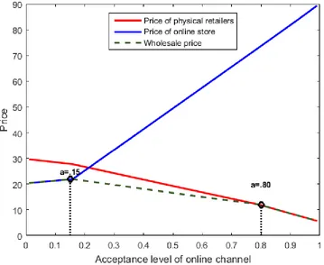
5.1. The impact of acceptance level of online channel (a) on pricing strategies

In this section, we analyze the effect of acceptance level of online channel (a) on the channel prices. In this example, to avoid the influence of other parameters, we consider five homogeneous competing retailers with a manufacturer-owned online store. In particular, we consider a supply chain with parameters:



5000, k_i .2,



30,



1, s_i 5, v_i 5,

=Uniform[0,100]

i

Figure 3. Impact of customer acceptance of online channel on prices

We conclude the influence of customer acceptance level on the sales network as follow: Managerial insight 1. Equilibrium results of the multiple-channel supply chain are stated as follow:

i. When the acceptance level of online store is lower than a threshold value and high percentage of potential customers prefer the physical retailers, the manufacturer to attract more customers should lower its price. However, a rational manufacturer would not cut the price below the wholesale price or the retailers may leave the market. Thus, the manufacturer sets the price of online channel equal to the wholesale price.

ii. For an interval range of the acceptance level of online store, the customers fairly prefer both the online store and traditional retailers. In this range, with increment of a, the manufacturer decreases the wholesale price to persuade the retailers to order more. The physical retailers decrease their price to attract more customers.

iii. For the high values of acceptance level of online store, the customers prefer to buy the product from online seller more greatly than the physical stores. In this case, the physical channels are not a serious threat to the online store and the manufacturer increases the price of online store. The physical retailers to attract customers would choosep_i w_i  i 1, 2,...,n, even with this pricing strategy, the physical retailers would not make any significant sales in the supply chain.

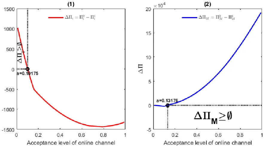
5.2. The impact of acceptance level of online channel (a) on profit functions

Let 2 1

1, 2,...,

i i i i n

       and 2 1

M M M

     represent the profit difference in two different scenarios for physical retailer i and the manufacturer, respectively.For the values of the parameter a that satisfy  i 0, physical retailer i is more profitable in a situation with no online channel while the manufacturer is more profitable in scenario 2 when  M 0 . We use the example of section 5.1 and Figure 4-1 and conclude the following managerial insight:

Managerial insight 2: When the acceptance level of online channel is lower than a threshold value, the physical retailers better off in presence of the new online store. The situation for the manufacturer is opposite and the new online store is beneficial to the manufacturer. Thus, the manufacturer can use the threshold value of a as a decision making criteria. The retailers also can use this parameter and decide whether to stay in the market or not.

Figure 4. Impact of customer acceptance of online channel on profit differences

5.3. Sensitivity analysis of model parameters on the Equilibrium

In this section a set of experiments is intended to analyze the sensitivity of the equilibrium point with respect to various parameters of the proposed model. It is assumed that the random part of demand function _i has the uniform distribution



_i Uniform



a b_i, _i



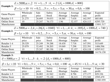
. In last part of the numerical analysis we report the equilibrium results for three different examples in the Table 1 and clarify them as follow:

i. The results of example 1 in Table 1 shows the equilibrium of the game in presence of 5

ii. The comparison of the results of examples 1 and 2 of Table 1 which only are different in the values of parameter k_i, that just changes the base market share of each physical retailer, shows that the optimal values related to the online store doesn’t change. The results of example 2 shows that the manufacturer chooses a higher wholesale price for the retailer with greater base market share (w_{1 4} 20.329w₅ 25.079 ). The sale price of physical retailer with higher base market share in the equilibrium is greater than other retailers’ prices.

iii. The comparison of the results of examples 1 and 3 of Table 1, which are different only in parameter ₀, shows that in situations that the price sensitivity of online store is high, the manufacturer sets a lower sale price for the online store to prevent losing the market share. Even with this pricing strategy the average sale of online store in example 1 is a lot more than with respect to example 3.

Table 1. Equilibrium of multiple- channel supply chain for different examples

Example 1:



0



5000, .2 1,...,5 : .2 1000, 800

1, 10 0, 2,...,5 : 5, = 5, 30, 0, 100

i i

i i i i i

a i k

c i v s a b











      

       

Game Players Wholesale price

Sale price

Safety Stock

Average Shortage

Average Surplus

Average sale

Expected profit Retailer 1-5 21.275 26.695 39.033 18.585 7.618 162.597 685.881 Online Store 10 25.247 76.173 1.96 32.157 424.113 6295.720

Manufacturer 15891.517

Example 2: 5



5





0



5000, .2, =.26 1040 1,..., 4 : .185 1000, 740

1, 10 0, 2,...,5 : 5, = 5, 30, 0, 100

i i

i i i i i

a k i k

c i v s a b













       

       

Game Players Wholesale price

Sale price

Safety Stock

Average Shortage

Average Surplus

Average sale

Expected profit Retailer 1-4 20.329 25.249 39.288 18.430 7.718 147.591 515.649 Retailer 5 25.079 32.492 38.203 19.049 7.298 222.391 1406.596 Online Store 10 25.247 80.196 1.96 32.157 424.118 6295.912

Manufacturer 16176.158

Example 3:



0



0 5000, .2 1,...,5 : .2 1000, 800

1, 10 0,1,...,5 : 5, = 5, 0, 100 45, 1, 2,..., 5 : 30

i i

i i i i i

a i k

c i v s a b i













      

          

Game Players Wholesale price

Sale price

Safety Stock

Average Shortage

Average Surplus

Average sale

Expected profit Retailer 1-5 20.097 26.003 41.942 16.854 8.796 177.177 829.336 Online Store 10 20.097 75.120 3.095 28.215 272.569 2595.479

Manufacturer 11983.959

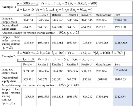
5.4. Impact of supply chain contracts on the multiple channel supply chain

However, the network profit is shared among all retailers and the manufacturer, depending on the retailers’ bargaining power, which is controlled by  in the coordinated supply chain model.

Table 2. The impact of supply chain contracts on players’ profit

Example 1:



0



5000, .2 1,...,5 : .2 1000, 800

1, 10 0, 2,...,5 : 5, = 5, 30, 0

i i

i i i i

a i k

c i v s a











      

      

Retailer 1 Retailer 2 Retailer 3 Retailer 4 Retailer 5 Manufacturer Sum Integrated

Supply chain 3445.54 3445.546 3445.546 3445.546 3445.546 5939.854 23167.585 Decentralized

supply chain 664.35 664.358 664.358 664.358 664.358 15891.51 19213.30 Acceptable range for revenue sharing contract: .192  .422

Supply chain under revenue sharing contract ( .3)

1033.664 1033.664 1033.664 1033.664 1033.664 17999.265 23167.585

Example 2:









5 5 0

5000, .2, =.24 1040 1,..., 4 : .19 1000, 760

1, 10 0, 2,...,5 : 5, = 5, 30, 0

i i

i i i i

a k i k

c i v s a













       

      

Retailer 1 Retailer 2 Retailer 3 Retailer 4 Retailer 5 Manufacturer Sum Integrated

Supply chain 3024.386 3024.386 3024.386 3024.386 5389.17 5939.824 23426.54 Decentralized

supply chain 563.571 563.571 563.571 563.571 1133.06 16018.01 19405.35 Acceptable range for revenue sharing contract: .328  .415

Supply chain under revenue sharing

contract ( .35)

1058.535 1058.535 1058.535 1058.535 1886.212 17306.191 23426.54

6. Conclusion

In this paper, we present a bi-level programming model to find the Stackelberg equilibria for wholesale and retail prices as well as order quantities for an online store in a multi-channel supply chain. The model reflects the price competition between traditional retailers and an online store in a supply chain. We formulated both centralized and decentralized supply chain situations and found the equilibrium points in both cases. In addition, we considered coordination in the model by applying a revenue sharing contract in order to decrease the amount of lost sales in the whole network. This contract enables the retailers to set their pricing and ordering policy the same as those in a centralized supply chain.

We conclude that offering the revenue sharing contract by the manufacturer would improve coordination in a multi-channel supply chain leading to higher profits for the entire network.

References

Bernstein, F., and Federgruen, A. (2004). "Dynamic inventory and pricing models for competing retailers", Naval Research Logistics (NRL), Vol. 51, No. (2), pp. 258-274.

Cachon, G. P. (2003). "Supply chain coordination with contracts", Handbooks in operations research and management science, Vol. 11, pp. 227-339.

Cai, G. G. (2010). Channel selection and coordination in dual-channel supply chains. Journal of Retailing, Vol. 86, No. 1, pp. 22-36.

Cattani, K., Gilland, W., Heese, H. S., and Swaminathan, J. (2006). "Boiling frogs: Pricing strategies for a manufacturer adding a direct channel that competes with the traditional channel", Production and Operations Management, Vol. 15, No. 1, pp. 40.

Chen, F. Y., Yan, H., and Yao, L. (2004). "A newsvendor pricing game", Systems, Man and Cybernetics, Part A: Systems and Humans, IEEE Transactions on, Vol. 34, No. 4, pp. 450-456. Chen, J., Zhang, H., and Sun, Y. (2012). "Implementing coordination contracts in a manufacturer Stackelberg dual-channel supply chain", Omega, 40(5), 571-583.

Chen, K.-Y., Kaya, M., and Özer, Ö. (2008). "Dual sales channel management with service competition", Manufacturing and Service Operations Management, 10(4), 654-675.

Dumrongsiri, A., Fan, M., Jain, A., and Moinzadeh, K. (2008). "A supply chain model with direct and retail channels", European Journal of Operational Research, 187(3), 691-718.

Kacen, J. J., Hess, J. D., and Chiang, W.-y. K. (2013). "Bricks or clicks? Consumer attitudes toward traditional stores and online stores", Global Economics and Management Review, 18(1), 12-21. Li, B., Chen, P., Li, Q., and Wang, W. (2014). "Dual-channel supply chain pricing decisions with a risk-averse retailer", International Journal of Production Research, 52(23), 7132-7147.

Liang, T.-P., and Huang, J.-S. (1998). "An empirical study on consumer acceptance of products in electronic markets: a transaction cost model", Decision support systems, 24(1), 29-43.

Moriarty, R. T., and Moran, U. (1990). "Managing hybrid marketing systems", Harvard Business Review, 68(6), 146.

Mukhopadhyay, S. K., Zhu, X., and Yue, X. (2008). "Optimal contract design for mixed channels under information asymmetry", Production and Operations Management, 17(6), 641-650.

Panda, S., Modak, N., Sana, S., and Basu, M. (2015). "Pricing and replenishment policies in dual-channel supply chain under continuous unit cost decrease", Applied Mathematics and Computation, 256, 913-929.

Petruzzi, N. C., and Dada, M. (1999). "Pricing and the newsvendor problem: A review with extensions", Operations Research, 47(2), 183-194.

Sayadi, M. K., and Makui, A. (2014). "Optimal advertising decisions for promoting retail and online channels in a dynamic framework", International Transactions in Operational Research, 21(5), 777-796.

Tsay, A. A., and Agrawal, N. (2004). "Channel Conflict and Coordination in the E‐Commerce Age", Production and Operations Management, 13(1), 93-110.

Yao, D.-Q., and Liu, J. J. (2005). "Competitive pricing of mixed retail and e-tail distribution channels", Omega, 33(3), 235-247.

Zhang, R., Liu, B., and Wang, W. (2012). "Pricing decisions in a dual channels system with different power structures", Economic Modelling, 29(2), 523-533.

Zhao, X. (2008). "Coordinating a supply chain system with retailers under both price and inventory competition", Production and Operations Management, 17(5), 532-542.

Zhao, X., and Atkins, D. R. (2008). "Newsvendors under simultaneous price and inventory competition", Manufacturing and Service Operations Management, 10(3), 539-546.

This article can be cited: Pakdel Mehrabani, R., and Seifi, A., (2018). "A bi-level programming approach to coordinating pricing and ordering decisions in a multi-channel supply chain", Journal of Industrial Engineering and Management Studies, Vol. 5, No. 2, pp. 13-37.

Appendix A.

Expected shortage and excess inventory are obtained as follows:

Expected shortage cost:

 

 





( ) ( )

( ) ( ) ( ) ( ) (1 ( ))

i i

i i

i i i i i i i i

b b

i i i i i i i i i i i i i i

z z

q E d q E p p z

z z f d f d z F z

  

     

 

      

  



 



 

By integration by parts, we would have the following:





( ) ( ) ( ) 1 ( )

( ) ( )

i i i i i i i i i i

i i i i i i

z z F z z z F z

z z z





      

     

Expected excess value:

 

 





( ) ( )

( ) ( ) ( ) ( ) ( )

i i i

i i i

i i i i i i i i

z z z

i i i i i i i i i i i i i i i

a a a

q E q d E p z p

z z f d z f d f d

  

       

 

      

  

_

 

_



_

By integration by parts, we would have the following:

( ) ( ) ( ) ( )

( ) ( ) i

i i

i

z

i i i i i i i i i i

a z

i i i i i

a

z z F z z F z F d

z F d









   

  





Appendix B.

Proof of Theorem 1.

According to Lemma 12 in Zhao and Atkins (2008), we need to show E[_i(p k_i, mp_i)]to bequasi-concave in p_i:

2







 





 







 



















 



2

E[ ( , )]

( )

E[ ( , )]

+ 1 E[ (

i i i i i i i i i i i i

i i i i

i i i

i i i i i i i

i

i i i i i i i

i

p k mp p k mp

v k mp

d p k mp

p k mp

dp

mp

p w p s

F k mp m v

w

F k mp

d

w

p w

w

 

  

        

   

  _{     }

   



 



































2 2

, )]

2 2 1

2 1

2

i i

i i i i i i i i

i

i i i i i i i i

p k mp

m F k mp m f k mp w v

dp

m F k mp mr k mp w v

p

p





 _{        }

  

     

(24)

If m 0 , then E[_i(p k_i, mp_i)] is strictly concave in p_i.

If m 0 , then let n   m 0. If



2mr ki



mpi



pi wi vi





0, then E[i(p ki, mpi)]

is strictly concave in p_i . Otherwise,



2mr k_i



mp_i



p_i w_i v_i





decreases as p_i increases. Hence

2

2

E[ _i( _i, _i)]

i

d p k mp

dp

 

either changes sign at most once from positive to negative or is always negative. Thus,

whenever E[ i( i, i)]

i

d p k mp

dp

 

turns negative, it remains negative, and E[_i(p k_i, mp_i)]is quasiconcave in p_i.So, function E[_i(p z_i, _i)] is quasiconcave in (p z_i, _i)and a pure-strategy Nash equilibrium exists.

Proof is complete.

Proof of Lemma 1. First we need to show that the optimization problem of retailer i , with p_i and z_ias decision variables, is convertible to an optimization problem over the single variablez_i . It is enough to verify that

E[_i(p z_i, _i)]is concave in p_i for a given z_i :









0

2

2

[ , ]

2 ( )

[ , ]

2 0

n

i i i j i

i i i

i i i i

i

i i

j j

i i

i

i

E p z

p z

p w p

p E p z

















  

  





  



 

 



(25)