Image Block Augmentation for One-Shot Learning

The Thirty-Third AAAI Conference on Artificial Intelligence (AAAI-19)

Image Block Augmentation for One-Shot Learning

Zitian Chen,

Yanwei Fu,

Kaiyu Chen,

Yu-Gang Jiang

3_{Shanghai Key Lab of Intelligent Information Processing, Fudan University,} {chenzt15, yanweifu,kychen15, ygj}@fudan.edu.cn

Abstract

Given one or a few training instances of novel classes, one-shot learning task requires that the classifier generalizes to these novel classes. Directly training one-shot classifier may suffer from insufficient training instances in one-shot learn-ing. Previous one-shot learning works investigate the meta-learning or metric-based algorithms; in contrast, this pa-per proposes a Self-Training Jigsaw Augmentation (Self-Jig) method for one-shot learning. Particularly, we solve one-shot learning by directly augmenting the training images through leveraging the vast unlabeled instances. Precisely our pro-posed Self-Jig algorithm can synthesize new images from the labeled probe and unlabeled gallery images. The labels of gallery images are predicted to help the augmentation process, which can be taken as a self-training scheme. In-trinsically, we argue that we provide a very useful way of directly generating massive amounts of training images for novel classes. Extensive experiments and ablation study not only evaluate the efficacy but also reveal the insights, of the proposed Self-Jig method.

Introduction

Inspired by the ability of people to acquire a new concept from a handful of examples, one-shot learning is recently studied with the goal of learning classifiers that general-ize to novel classes which only have one, or a few training instances of each class. While this problem is quite diffi-cult, the main obstacle is lacking enough training images in the novel classes. To address this task, previous efforts ex-plored transferring knowledge from source base classes to help learn a classifier on target novel classes, by the ways of meta-learner (Vinyals et al. 2016; Snell, Swersky, and Zemeln 2017) or metric space(Finn, Abbeel, and Levine 2017; Zhou, Wu, and Li 2018; Li et al. 2017), and to a lesser extent, data augmentation in novel classes (Wang et al. 2018; Hariharan and Girshick 2017).

In term of Gestalt principles of perceptual grouping (Des-olneux, Moisan, and Morel 2004), humans can naturally per-ceive objects as the organized patterns and objects. People have been entertained by solving Jigsaw puzzles by assem-bling the pieces into a complete picture. In this game, even though some pieces are missing, we are still able to infer the

Copyright © 2019, Association for the Advancement of Artificial Intelligence (www.aaai.org). All rights reserved.

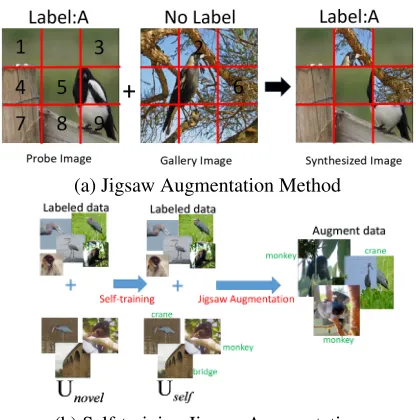
(a) Jigsaw Augmentation Method

(b) Self-training Jigsaw Augmentation

Figure 1: Illustration of our augmentation method. The syn-thesized image is visually consistent in each block (i.e.,local consistent), but not in all blocks (i.e.,not global consistent).

content drawn in Jigsaw. This game thus inspires us a totally different way of addressing one-shot learning by replacing some pieces of labeled images and producing the deformed additional images to help train the one-shot classifier.

augmentation method can synthesize new image by replac-ing some blocks. The synthesized images can then be uti-lized to update the classifiers in the target domain. Critically, we present a very effective way of directly generating a large number of training images in the novel classes. The whole pipeline of our method is illustrated in Fig. 1(b). Remark-ably, our framework is orthogonal and complementary to all previous one-shot methods (Finn, Abbeel, and Levine 2017; Zhou, Wu, and Li 2018; Li et al. 2017; Vinyals et al. 2016); and the augmented training images, in principle, can be uti-lized to train classifiers in the target domain. Extensive ex-periments show that our framework can greatly improve the one-shot learning performance.

Related Work

We briefly review the connections and differences between our method with several related works. Note that the litera-ture on these topics is vast, only works that most relevant are summarized here.

One-Shot Learning.Previous works explored it by metric-learning and meta-metric-learning. The former one aims at metric-learning a metric space in which the one-shot classification can be performed. The recent typical works on metric learning in-clude Deep Siamese Networks(Koch, Zemel, and Salakhut-dinov 2015), Matching Nets (Vinyals et al. 2016), PROTO-NET (Snell, Swersky, and Zemeln 2017), RELATION PROTO-NET (Sung et al. 2018) and MACO (Hilliard et al. 2018). The meta-learning algorithms (Finn, Abbeel, and Levine 2017; Li et al. 2017; Zhou, Wu, and Li 2018; Ravi and Larochelle 2017; Munkhdalai and Yu 2017; Wang and Hebert 2016) train a “high-level meta-structure” – meta-learner to fast op-timize and adapt the weights of low-level networks. Ad-ditionally, other strategies have also been investigated in one-shot learning, such as attention (Wang et al. 2017; Guttenberg and Kanai 2018), graph CNN (Garcia and Bruna 2018), and memory network (Santoro et al. 2016; Cai et al. 2018). Different from all these works, our model directly generates synthesized images for one-shot classes; thus is orthogonal and complementary to all these previous works.

Data Augmentation. In standard supervised classifica-tion, researchers usually utilize many data augmentation methods, such as flipping, rotating, adding noise and ran-domly cropping images, to train deep networks (Krizhevsky, Sutskever, and Hinton 2012; Chen et al. 2018; Zeiler and Fergus 2014). More advanced augmentation method is to synthesize or edit images directly, by hallucinating (Wang et al. 2018), shrinking and hallucinating features (Hariharan and Girshick 2017), mixing paring samples (Inoue 2018), or randomly erasing parts of images (Zhong et al. 2017). Quite differently, our Jigsaw augmentation dynamically syn-thesizes the new image by integrating two images: one is the labeled image, the other one is selected from the unlabeled image set by self-training scheme. Thus visually our new image can be both similar and yet significant different to the labeled image.

Semi-supervised Learning.It focuses on facilitating unla-beled data to help learn classifiers, particularly by deep ar-chitectures (Rasmus et al. 2015; Laine and Aila 2016). These

works nevertheless still require an amount of labeled data to initially train a deep network, thus limited in the one-shot learning scenario. Recently, Renet al.(Ren et al. 2018) ad-dressed the semi-supervised few-shot learning tasks by ex-tending PROTO-NET (Snell, Swersky, and Zemeln 2017). In contrast, our model primarily targets at augmenting train-ing data by the proposed self-traintrain-ing Jigsaw augmenta-tion model, which is also very different from standard self-training scheme (Yarowsky 1995; Chuck Rosenberg 2005). That is, our framework utilizes the self-training scheme to select unlabeled images as the gallery images to help syn-thesize new images by Jigsaw augmentation method.

Image Block Augmentation

In one-shot learning, we are given the base categoriesCbase, and novel categoriesCnovel in the source/target domain re-spectively. The Cbase have sufficient labeled image data

Dbase = {Ii, yi},yi ∈ Cbase. We conduct one-shot learn-ing on theCnovel which only have a small amount of la-beled dataDnovel = {Ii, yi},yi ∈ Cnovel ; additionally, we have large amounts of unlabeled data of novel categories

Unovel ={Iu}in the target domain.

Our framework has two steps. We firstly use base classes to train the base network, which is further fine-tuned as the robust feature extractor by the augmented data, generated by our Jigsaw augmentation method. We further employ the augmentation method on novel classes by using unlabeled data to help train the classifier for one-shot recognition.

Jigsaw Augmentation Method to Synthesize Images

We introduce a novel Jigsaw data augmentation method. As Fig. 1(a), all the images are resized to the same fixed size, and divided into nine blocks. Some blocks ofprobe image

Iiare randomly chosen and replaced bymblocks (m≤4) of corresponding positions fromgallery imageIu.

Generally, we require Ii andIu to have the same class label. However, in target domainCnovel, the gallery image

Iu is unlabeled; thus we use the predicted label of Iu by self-training scheme. Such a way has several benefits.

First, when the class label of Iu is very different from that of Ii, (i.e., the labels ofIu is wrongly predicted), the synthesized imageeIi can be taken as the randomly erased version of Ii. Interestingly such synthesized imageeIi has been shown in (Zhong et al. 2017) to be able to improve the generalization ability of the deep network, and complemen-tary to the classical augmentation techniques,e.g., random cropping, and flipping.

Learning Robust Feature Extractor of Base Classes

To learn a feature extractor, we firstly train base network on

Dbase, and then fine-tune the base network with synthesized images generated by Jigsaw augmentation method, which replaces some blocksm ≤4. Particularly, we use the base categoriesCbaseto train a supervised classification network

f(I;θ);θindicates the parameter set. Thef(I;θ)can be a classification network, e.g., ResNet (He et al. 2015). In

Dnovel, we can use the final layer output of f(I;θ)as the extracted features of the imageI.

Thef(I;θ)should be trained to robustly extract the fea-tures of the synthesized image setneIi

o

which is locally

con-sistent, but not globally. Thus, we fine-tune thef(I;θ)by the synthesized images from synthesized image set Debase until converged. To construct the synthesized image set

e

Dbase, the probeIiand galleryIuimages are randomly sam-pled fromDbase. We want to highlight several issues with this fine-tuning step.

Firstly, rather than using onlyDebaseto fine-tunef(I;θ), we actually mixDebaseandDbaseto avoid the “catastrophic

forgetting” of the network (McCloskey and Cohen 1989). Otherwise, the fine-tuned network will be inclined to extract robust features of images inDebase, but notDbase.

Secondly, training by the augmented setDebase does not improve the classification performance of f(I;θ) on the source domain. This is very reasonable, since the gallery images that generateDebasehave already been used to train

f(I;θ).In other words, any each block of newly synthesized imageeIiinDebase has been trained inf(I;θ); and there is no new information being learned. This motivates our semi-supervised framework of using unlabeled image setUnovel to help one-shot learning. Thus oncef(I;θ)is trained, we use it as the generic feature extractor for one-shot recogni-tion.

Thirdly, Norooziet al. (Noroozi and Favaro 2016) took solving Jigsaw puzzles as a pretext task to train a context-free network in boosting the performance of object classifi-cation and detection. In contrast, our fine-tuning step intro-duced here can be used in any base network rather than the specially designed network as in (Noroozi and Favaro 2016). Furthermore, the target of our fine-tuning step is only to teach the network to understand the synthesized images, rather than directly boosting the performance of one-shot classification.

Self-Training Jigsaw Augmentation Algorithm

We explain our self-training Jigsaw augmentation algorithm in details. Particularly, in novel categories, the we can ex-tract the features x = f(I;θ)of image I ∈ Dnovel; and we further train a classifierg(x;η)with the parameter set

η. The classifierg(·)can either be Support Vector Machine (SVM), Logistic Regression (LR) or Neural Network. The

g(x;η)is directly applied toUnovel to predict the class la-bel of each image Iu. Among these unlabeled images, the

g(x;η)selects the image subsetUself = {Iu} ⊆ Unovel of high prediction confidence, as well as the corresponding

label setyself ={g(f(Iu;θ) ;η)}.

We then apply the Jigsaw augmentation method by tak-ingDnovel andUself as probe and gallery set respectively. We set the replacing blockm ≤ 2. Specifically, given one labeled image Ii as the probe image, we randomly select one gallery image Iu ∈ Uself, conditioning that yi =

g(f(Iu;θ) ;η). We can thus generate the augmented dataset

e Dnovel=

n e

Ii, yi

o

by Jigsaw augmentation method. In

one-shot recognition, we use the networkf(I;θ)to extract the image features of Dnovel andDenovel and train the classi-fier_eg(x;η), which can be applied to categorize the testing instances.

Intrinsically, our algorithm can indeed use the self-training scheme (Chuck Rosenberg 2005) of updating

g(x;η), which is one of the simplest semi-supervised algo-rithms. Note that traditional self-training algorithm may suf-fer from the semantic drift by reinforcing poor predictions. In contrast, the synthesized images generated by our Jig-saw augmentation algorithm may have better performance in learning the one-shot learning models. This is because the synthesized images can be either the cropped labeled probe images or semantically composed images. Note that it is useless to synthesizing new images by simply exchang-ing blocks between labeled images due to that does not brexchang-ing in any new information. This point is also evaluated in our ablation study of the experiments.

Experiments

Extensive experiments are conducted onminiImageNet and ImageNet1k challenge datasets. The codes and models will be released upon acceptance.

The miniImageNet proposed in (Vinyals et al. 2016), is one of the most widely used benchmark dataset on one-shot learning. It has 60,000 images from 100 classes with 600 images per class. The data split setup is used by (Ravi and Larochelle 2017) with 64, 16, 20 classes as training vali-dation, and testing set individually. Only the 64 classes of training set serve as theCbaseto train feature extractor. As in (Vinyals et al. 2016; Ravi and Larochelle 2017), we consider 1-shot and 5-shot classification for five classes asCnovel ran-domly chosen from testing class set; and 15 examples per class for evaluation in each test round. The results are av-eraged and reported over multiple rounds. Additionally, in each round, we randomly select, 30 unlabeled images per class (Unovel ) that have not used for training and testing. We employ a self-training scheme to select half of the im-ages fromUnovelasUself.

We also conduct the experiments on the large-scale dataset – ImageNet1k challenge dataset. We use the same splitCbase andCnovel as proposed in (Hariharan and Gir-shick 2017). The Top-1 and Top-5 accuracy are reported. The results are averaged over 5 repeated runs as (Hariharan and Girshick 2017). On each novel category, we randomly sample 50 images per class as the unlabelled setUnovel.

Methods n=1 2 5 10 20

Baselines

Softmax –/14.1 –/33.3 –/56.2 –/66.2 –/71.5

LR 18.3/42.8 26.0/54.7 35.8/66.1 41.1/71.3 44.9/74.8

SVM 15.9/36.6 22.7/48.4 31.5/61.2 37.9/69.2 43.9/74.6

Competitors

Matching Network](Vinyals et al. 2016) –/43.0 –/54.1 –/64.4 –/68.5 –/72.8 Model Regression](Wang and Hebert 2016) 16.9/41.7 24.0/53.6 33.5/63.7 37.7/68.2 42.7/72.3 Generation-SGM (Hariharan and Girshick 2017) –/34.3 –/48.9 –/64.1 –/70.5 –/74.6

Flipping 17.4/39.6 24.7/51.2 33.7/64.1 38.7/70.2 44.2/74.5

Gaussian Noise 16.8/39.0 24.0/51.2 33.9/63.7 38.0/69.7 43.8/74.5

Gaussian Noise(feature level) 16.7/39.1 24.2/51.4 33.4/63.3 38.2/69.5 44.0/74.2

Ours

Self-Jig (SVM)* 23.8/51.9 31.5/62.1 38.6/69.6 42.4/73.2 45.8/75.7

Self-Jig(SVM)+ 17.7/39.1 24.9/51.3 34.1/64.9 39.1/70.6 44.2/74.9

Self-Jig (LR)* 22.0/49.3 30.1/60.5 38.1/68.7 41.9/72.2 44.9/74.9

Self-Jig (LR)+ 20.1/45.3 28.1/56.9 36.5/66.4 41.3/71.5 44.8/74.6

Ablation Study I

Rob (LR) 16.7/40.5 24.2/52.5 33.7/64.2 38.9/69.4 43.1/73.0

Jigsaw (LR) 17.5/42.2 25.1/53.9 33.9/64.7 39.8/67.9 41.3/70.6

Self-T (LR) 16.1/41.2 24.6/52.9 32.8/64.0 39.7/68.8 42.2/72.7

Rob (SVM) 14.3/33.2 20.5/44.4 29.4/58.6 36.3/67.5 42.0/72.9

Jigsaw (SVM) 14.2/33.9 20.1/45.2 29.2/58.4 34.1/65.1 40.0/68.4

Self-T (SVM) 16.0/36.7 22.7/48.4 30.8/60.0 35.7/66.7 40.9/69.5

Ablation Study II

Rob+Jigsaw (LR) 22.1/47.2 29.3/57.0 36.1/66.3 41.0/71.1 44.5/74.1 Rob+Self-T (LR) 16.3/41.5 24.4/52.7 33.1/64.1 39.9/69.2 42.6/72.5 Self-T+Jigsaw (LR) 15.6/40.3 23.6/51.8 32.0/63.5 39.1/68.5 41.9/71.8 Rob+Jigsaw (SVM) 17.9/37.0 23.9/48.3 29.5/58.8 35.1/65.7 40.3/68.8 Rob+Self-T (SVM) 15.0/35.5 21.8/47.5 29.9/59.2 34.6/65.4 39.8/68.3 Self-T+Jigsaw (SVM) 13.1/31.9 19.0/44.3 28.3/57.2 33.0/64.3 39.1/67.2

Table 1:Top-1 / Top-5 results of Imagenet1K (ResNet-10).*: our methods.]: results from (Hariharan and Girshick 2017).+ : Jigsaw is applied inDbaserather thanUnovel(fromDnovel).

Setup. To make a comparison to (Hariharan and Girshick 2017), we choose both ResNet-10 and ResNet-50 resid-ual network (He et al. 2015) as the base networks to train

f(I;θ). For both networks, we use SGD to train networks which gets converged in 300 epochs: the learning rate is set to1×10−1 _{and degraded by 10 every 30 epochs with} the batch size 128. We augment each training instance up to five instances and train for 10 epochs.In fine-tuning, each probe imageIihelps produce 10 synthesize imageeIiand we trained for 10 epochs. The learning rate of the last layer and the other layers are set to1×10−1_,1×10−2_respectively in our experiments.

Baselines and competitors. As the naive baselines, we di-rectly use Cbase to train f(I;θ) which serves as the fea-ture extractor to extract feafea-turexof the imageI; and further train g(x;η). Theg(x;η)can be used as Support Vector Machine (SVM), Logistic Regression (LR) or Neural Net-work of 1 fully connected layer and 1 Softmax classification layer (Softmax). In our experiments, SVM and LR perform consistently better than Softmax, and thus are further used in the ablation study. We also compare with recent models, such as Model Regression (Wang and Hebert 2016), Match-ing Network (Vinyals et al. 2016), Generation SGM (Hari-haran and Girshick 2017). The standard data augmentation methods are also compared here: “Flipping”: the same in-put image is flipped from left to right; “Gaussian Noise”:

we add Gaussian noise N(0,10) to each pixel of the in-put image; “Gaussian Noise (feature level)”: the Gaussian noiseN(0,0.3)is also added to each dimension of ResNet-18 feature extracted of each image. To make fair compar-isons, all the augment methods utilize the SVM classifier as the one-shot classifier.

Variants of our framework. An ablation study is used to evaluate these three components of our framework: (1) Learning robust feature extractor (“Rob”): we only learn robust feature extractor, and directly apply the feature ex-tractor to do one-shot classification on Cnovel; (2) Self-training scheme (“Self-T”): we only use Dbase to train

f(I;θ); and onCnovel, we apply the self-training method (Chuck Rosenberg 2005) to update the classifierg(x;η); (3) Jigsaw data augmentation (“Jigsaw”): we only useDbaseto train f(I;θ); and we randomly select some unlabeled im-ages as the gallery imim-ages in Jigsaw augmentation to get

e

Dnovelandeg(x;η).

Figure 2: t-SNE Visualization. Stars, Circles and Triangles represent the labeled probe, unlabeled gallery, and synthesized image produced by our framework.

Figure 3: Top 5 accuracy(%) on Imagenet1K (Resnet-10).

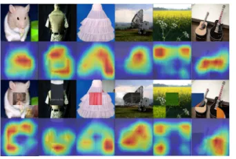
Figure 4: Class activation of probe and synthesized images.

(2) On Top-5 accuracy, our Self-Jig (SVM) can beat the best competitors – Matching Network (Vinyals et al. 2016) by more than10% in Tab. 1. The same conclusion still holds when we use the ResNet-50 in Tab. 2. We argue that much of our success and improvement comes from a more dis-criminative augmented training setDenovel by self-training Jigsaw augmentation method, rather than from the other fac-tors, since the Self-Jig (SVM) can beat the corresponding baselines and competitors by a large margin both in Tab. 1 and Tab. 2.

(3) We found that due to the small number of training in-stances onCnovel , the Softmax classifier has lower

recog-Methods n=1 2 5 10

Softmax –/28.2 –/51.0 –/71.0 –/78.4

SVM 20.1/41.6 29.4/57.7 42.6/72.8 49.9/79.1

LR 22.9/47.9 32.3/61.3 44.3/73.6 50.9/78.8

Generation SGM –/47.3 –/60.9 –/73.7 –/79.5 Self-Jig (SVM) 30.3/59.7 39.7/70.9 48.7/78.7 51.1/80.3 Self-Jig (LR) 32.8/62.8 41.2/71.3 49.2/77.9 51.5/79.3 Robust (SVM) 19.2/40.7 28.3/56.6 41.4/71.9 48.7/77.9 Robust (LR) 21.8/46.5 31.2/60.2 43.3/72.6 50.7/77.5

Table 2: Top-1 / Top-5 accuracy on Imagenet1K Chal-lenge Dataset (ResNet-50).Self-Jig (LR)indicates that LR classifier is used as g(I;η). Self-T: self-training; Jigsaw: Jigsaw Augmentation. Rob: Robust feature extractor. n in-dicates the number of training instances per class.

nition accuracy than SVM and LR. Fig.3 clearly visualize the performances of three different classifiers when chang-ing the number of trainchang-ing instances.

We further extend the experiments in few-shot settings by increasing the training instances from 1 to 20 as shown in Tab. 1 and Tab. 2 . We found that our methods can still beat the other baselines and competitors, due to the fact that our augmented training instance set can help train the classifier onCnovel. We also observe that the improvements achieved by our self-training Jigsaw augmentation method tend to somewhat diminish as the number of training in-stances substantially grows from 1, 2, 5 to 20 shots. This also makes sense. With sufficient training instances, the classifier

g(I;η)can be better learned and the effects of augmenting labeled images from the unlabeled set Uself, become less pronounced.

Ablation study. In Ablation Study I in Tab. 1, we evalu-ate the variants of our model. Here when we use Jigsaw without self-T, means we synthesized new images from the probe and randomly selected gallery images. We note that, (1) almost all the results of using each single component get degraded than the naive baselines. (2) Self-T (SVM) and Self-T (LR) are the naive semi-supervised baselines by the self-training method only. They add the most confidence in-stances fromUnovel to update the corresponding classifier

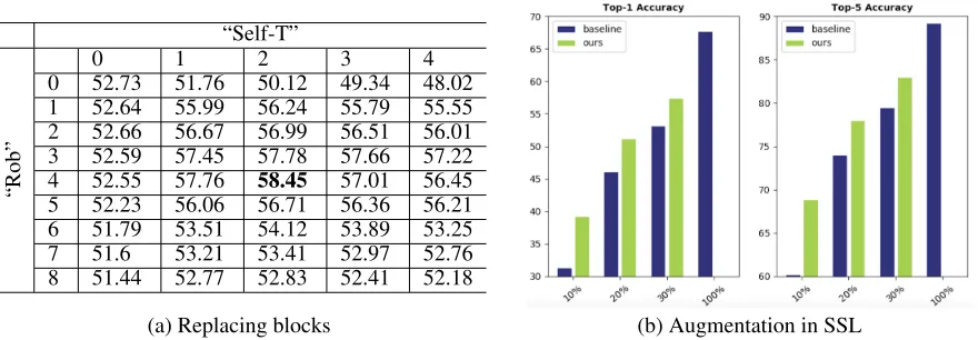
“Self-T”

“Rob”

0 1 2 3 4

0 52.73 51.76 50.12 49.34 48.02

1 52.64 55.99 56.24 55.79 55.55

2 52.66 56.67 56.99 56.51 56.01

3 52.59 57.45 57.78 57.66 57.22

4 52.55 57.76 58.45 57.01 56.45

5 52.23 56.06 56.71 56.36 56.21

6 51.79 53.51 54.12 53.89 53.25

7 51.6 53.21 53.41 52.97 52.76

8 51.44 52.77 52.83 52.41 52.18

(a) Replacing blocks (b) Augmentation in SSL

Figure 5: (a)Each row/column is corresponding to the number of replaced blocks in the “Rob”/”Self-T” component individually. The 1-shot classification accuracy onCnovel are reported. (b) Our Self-Jig is used in semi-supervised learning. The X-axis indicates the number of percentage of training instances used. Y-axis denotes the classification accuracy.

can get slightly improved over SVM method, due to discrim-inative information learned from unlabeled data. Critically, this shows that the proposed methodology is a single uni-fied framework; and the significant improvement of Self-Jig comes from the integration of all three components, rather than each individual component.

In Ablation Study II in Tab. 1, the combinations of two components are compared. Interestingly, (1) we found that using two components can indeed help improve the perfor-mance over the corresponding baselines. For example, the “Rob+Jigsaw (LR)” and “Rob+Jigsaw (SVM)” have better classification accuracy over the LR and SVM baselines, but lower results than our Self-Jig (LR) and Self-Jig (SVM). This actually demonstrates that the importance of “self-training” component in selecting theUselffor data augmen-tation. (2) Additionally, the SVM classifier is more sensitive to the quality of training instances than LR. With the aug-mented dataDenovelby our self-training Jigsaw method, our Self-Jig (SVM) have better performance than Self-Jig (LR). In contrast, Ablation study I and Ablation Study II show that the baseline methods by SVM classifiers are significantly lower than those corresponding variants by the LR classi-fier, due to the small number or low augmented data quality of training instances.

Without unlabeled data.Our framework still works with-out access to the extra unlabeled data. We could sample in-stances fromDbase to serve as the gallery images. In this case, the Jigsaw Augmentation is conducted between im-ages from different categories but likely to have a similar appearance. As shown in Tab. 1, we observed marginally improved (Self-Jig(SVM)+,Self-Jig(LR)+) over the naive baseline (SVM,LR).

Results on

mini

ImageNet

Setup.We employ ResNet-18 structure as the feature extrac-torf(I;θ). By default, we use the same hyperparameter and experimental settings as we train the network in ImageNet1k challenge dataset.

Competitors. As in Tab. 3, we mainly compare three

groups of the competitors: Meta-learning algorithms, such as MAML (Finn, Abbeel, and Levine 2017), Meta-SGD (Li et al. 2017), DEML+Meta-SGD (Zhou, Wu, and Li 2018), META-LEARN LSTM (Ravi and Larochelle 2017) and Meta-Net (Munkhdalai and Yu 2017); Metric-learning algorithms, such as Matching Nets (Vinyals et al. 2016), PROTO-NET (Snell, Swersky, and Zemeln 2017), RELA-TION NET (Sung et al. 2018), and MACO (Hilliard et al. 2018)) ; and other semi-supervised methods, including Semi-supervised PROTO-NET (S.S. PROTO-NET) (Ren et al. 2018), Ladder Network (Rasmus et al. 2015), Graph Neu-ral Networks(Garcia and Bruna 2018), Transductive Prop-agation Network(Liu et al. 2018), Semi-supervised Resnet PN(Boney and Ilin 2017). In particular, to make a fair com-parison, we implement the ladder network by using ResNet-18 architectures and the Graph Neural networks under same settings. Random Erase (Zhong et al. 2017) is the method that randomly erases the images. We implement the method (Zhong et al. 2017) by ResNet-18 with SVM classifier.

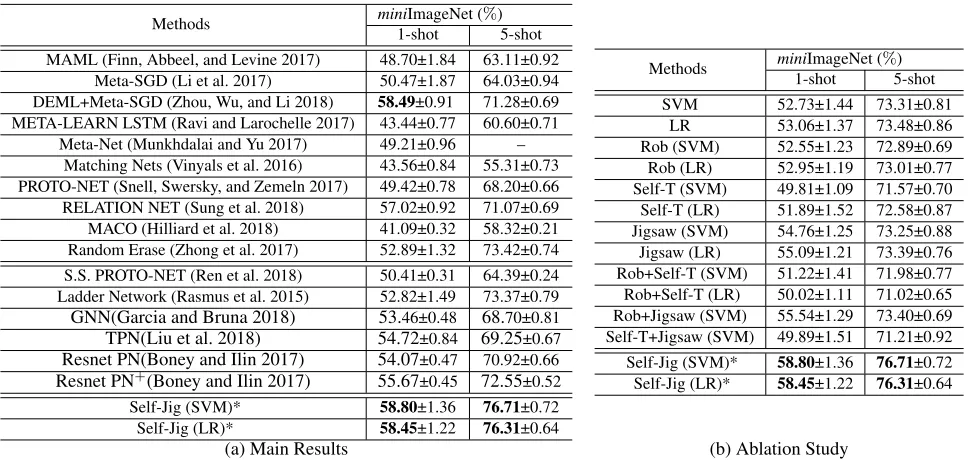
Results.As shown in Tab. 3(a), our Self-Jig (SVM) achieves the best performance in the 1-shot and 5-shot classification settings. This validates the effectiveness of our framework in using the unlabeled images in data augmentation. Further-more, we split the proposed framework, and evaluate each component/the combination of any two components in Tab. 3(b). We have two conclusive results: (1) Our frameworks,

i.e., Self-Jig (SVM), and Self-Jig (LR), get significantly im-proved over the corresponding baselines – SVM and LR, on 1-shot and 5-shot classification. This again shows the effi-cacy of our self-training Jigsaw data augmentation in help-ing one-shot classification. (2) The variants of only ushelp-ing each or any two components have no or very limited im-provement over the corresponding baselines. That indicates that the proposed method is a unified single framework.

Methods miniImageNet (%)

1-shot 5-shot

MAML (Finn, Abbeel, and Levine 2017) 48.70±1.84 63.11±0.92 Meta-SGD (Li et al. 2017) 50.47±1.87 64.03±0.94 DEML+Meta-SGD (Zhou, Wu, and Li 2018) 58.49±0.91 71.28±0.69 META-LEARN LSTM (Ravi and Larochelle 2017) 43.44±0.77 60.60±0.71

Meta-Net (Munkhdalai and Yu 2017) 49.21±0.96 – Matching Nets (Vinyals et al. 2016) 43.56±0.84 55.31±0.73 PROTO-NET (Snell, Swersky, and Zemeln 2017) 49.42±0.78 68.20±0.66 RELATION NET (Sung et al. 2018) 57.02±0.92 71.07±0.69 MACO (Hilliard et al. 2018) 41.09±0.32 58.32±0.21 Random Erase (Zhong et al. 2017) 52.89±1.32 73.42±0.74

S.S. PROTO-NET (Ren et al. 2018) 50.41±0.31 64.39±0.24 Ladder Network (Rasmus et al. 2015) 52.82±1.49 73.37±0.79

GNN(Garcia and Bruna 2018) 53.46±0.48 68.70±0.81

TPN(Liu et al. 2018) 54.72±0.84 69.25±0.67

Resnet PN(Boney and Ilin 2017) 54.07±0.47 70.92±0.66

Resnet PN+(Boney and Ilin 2017) 55.67±0.45 72.55±0.52

Self-Jig (SVM)* 58.80±1.36 76.71±0.72

Self-Jig (LR)* 58.45±1.22 76.31±0.64

Methods miniImageNet (%)

1-shot 5-shot

SVM 52.73±1.44 73.31±0.81

LR 53.06±1.37 73.48±0.86

Rob (SVM) 52.55±1.23 72.89±0.69 Rob (LR) 52.95±1.19 73.01±0.77 Self-T (SVM) 49.81±1.09 71.57±0.70 Self-T (LR) 51.89±1.52 72.58±0.87 Jigsaw (SVM) 54.76±1.25 73.25±0.88 Jigsaw (LR) 55.09±1.21 73.39±0.76 Rob+Self-T (SVM) 51.22±1.41 71.98±0.77 Rob+Self-T (LR) 50.02±1.11 71.02±0.65 Rob+Jigsaw (SVM) 55.54±1.29 73.40±0.69 Self-T+Jigsaw (SVM) 49.89±1.51 71.21±0.92

Self-Jig (SVM)* 58.80±1.36 76.71±0.72 Self-Jig (LR)* 58.45±1.22 76.31±0.64

(a) Main Results (b) Ablation Study

Table 3: Results onminiImageNet. The “±” indicates95%confidence intervals over tasks. *: indicates our method.

unlabeled images per category respectively, while our method use 15. As in Tab. 3(a), our frameworks easily over-perform other methods in both 1-shot and 5-shot classifica-tion settings.

Visualization. We visualize the Class Activation Map (CAM) of images in Fig. 4. Specifically, the first and third rows are labeled probe and synthesized images produced by our framework, respectively. The second and fourth rows are the activation map computed from the first and third rows by (Zhou et al. 2015) individually. In particular, the high-est predicted class scores of each image is projected back to highlight its class–specific discriminative regions. We can show that if the replaced blocks of the synthesized images are highly related to its class label, the class-specific region would be enlarged, such as the “radar” image in the fourth column; otherwise, this region will be reduced.

To give more insights we visualize five classes in Fig. 2(a). The Stars, Circles, and Triangles represent the labeled probe, the unlabeled gallery, and the synthesized image gen-erated by our framework. The instances of each class are de-noted by the same color. We can see in Fig. 2(a) that most of our synthesized images (i.e., Triangles) are still in the same class manifold. This explains why our synthesized images can help a lot in one-shot classification. We show the in-stances distribution of the red (Fig. 2(b)), green (Fig. 2(c)) and purple class (Fig. 2(d)) of Fig. 2(a). Each pair of labeled probeIi , unlabeled galleryIuand synthesized imageeIi is drawn with the same color. We can observe that when the gallery image is on the same manifold as probe image, the synthesized image is also on the manifold,e.g., the blue pair in Green class in Fig. 2(c) .

Ablation Study

We conduct extensive further ablation study on

miniImageNet to reveal the insights of our framework. In particular, we answer several questions as follows,

Replacing blocks.We use Jigsaw augmentation to fine-tune the base network withm≤4; The “Self-T” component em-ploys the Jigsaw augmentation (m ≤ 2) in a self-training manner. We vary the parameter m in our framework and compare the results in Tab. 5. We can see that by chang-ing the number of replaced blocks, there may be a slight variance in one-shot classification accuracy; but, our experi-mental conclusions still hold.

The Number of synthesized images.We choose to generate 10 synthesized images in our experiments. We also compare the results of generating 0, 1, 2, 5, 10, 20, 50, 100, 200, 500, 1000 synthesized images, while all the other parameters are kept the same. Thus the corresponding one-shot classifica-tion accuracies are 52.55%, 55.84%, 57.14%, 57.9%, 58.2%, 58.02%, 57.96%, 58.42%, 58.24%, 58.11% and 58.19%, re-spectively. Thus, we found that changing this parameter may lead to a slight variance of the final performance. But our fi-nal results are still significantly better than the baselines.

Performance in Semi-Supervised Learning (SSL). Our Self-Jig is tested in the SSL setting onCbaseclasses: we use

Conclusion

This work proposes a self-training Jigsaw data augmentation method for one-shot learning. Extensive experiments show the efficacy of our framework in synthesizing new instances to boost the recognition performance.

Acknowledgments

This work was supported in part by National Key R&D Program of China (#2017YFC0803700), NSF China (#U1611461, #61622204, #61572138, #61702108), and STCSM (#16JC1420400, #17JC1401600). Dr. Yanwei Fu is the corresponding authour.

References

Boney, R., and Ilin, A. 2017. Semi-supervised few-shot learning with prototypical networks.CoRRabs/1711.10856. Cai, Q.; Pan, Y.; Yao, T.; Yan, C.; and Mei, T. 2018. Memory Matching Networks for One-Shot Image Recognition. Chen, Z.; Fu, Y.; Zhang, Y.; Jiang, Y.-G.; Xue, X.; and Si-gal, L. 2018. Semantic Feature Augmentation in Few-shot Learning.ArXiv e-prints.

Chuck Rosenberg, Martial Hebert, H. S. 2005. Semi-supervised self-training of object detection models. InIEEE workshop on Motion and Video Computing.

Desolneux, A.; Moisan, L.; and Morel, J.-M. 2004. Gestalt theory and computer vision. InTheory and Decision Library A:.

Finn, C.; Abbeel, P.; and Levine, S. 2017. Model-agnostic meta-learning for fast adaptation of deep networks. In

ICML.

Garcia, V., and Bruna, J. 2018. Few-Shot Learning with Graph Neural Networks. InICLR.

Guttenberg, N., and Kanai, R. 2018. Learning to generate classifiers.ArXiv e-prints.

Hariharan, B., and Girshick, R. 2017. Low-shot visual recognition by shrinking and hallucinating features. In

ICCV.

He, K.; Zhang, X.; Ren, S.; and Sun, J. 2015. Deep residual learning for image recognition. InCVPR.

Hilliard, N.; Phillips, L.; Howland, S.; Yankov, A.; Corley, C. D.; and Hodas, N. O. 2018. Few-Shot Learning with Metric-Agnostic Conditional Embeddings. ArXiv e-prints. Inoue, H. 2018. Data Augmentation by Pairing Samples for Images Classification.ArXiv e-prints.

Koch, G.; Zemel, R.; and Salakhutdinov, R. 2015. Siamese neural networks for one-shot image recognition. InICML – Deep Learning Workshok.

Krizhevsky, A.; Sutskever, I.; and Hinton, G. E. 2012. Imagenet classification with deep convolutional neural net-works. InNIPS.

Laine, S., and Aila, T. 2016. Temporal Ensembling for Semi-Supervised Learning.

Li, Z.; Zhou, F.; Chen, F.; and Li, H. 2017. Meta-sgd: Learning to learn quickly for few shot learning. In

arxiv:1707.09835.

Liu, Y.; Lee, J.; Park, M.; Kim, S.; and Yang, Y. 2018. Trans-ductive propagation network for few-shot learning. CoRR

abs/1805.10002.

McCloskey, M., and Cohen, N. J. 1989. Catastrophic inter-ference in connectionist networks: The sequential learning problem.Psychology of learning and motivation.

Munkhdalai, T., and Yu, H. 2017. Meta networks. InICML. Noroozi, M., and Favaro, P. 2016. Unsupervised learning of visual representations by solving jigsaw puzzles. InECCV. Rasmus, A.; Valpola, H.; Honkala, M.; Berglund, M.; and Raiko, T. 2015. Semi-supervised learning with ladder net-works. InNIPS.

Ravi, S., and Larochelle, H. 2017. Optimization as a model for few-shot learning. InICLR.

Ren, M.; Triantafillou, E.; Ravi, S.; Snell, J.; Swersky, K.; Tenenbaum, J. B.; Larochelle, H.; and Zemel, R. S. 2018. Meta-learning for semi-supervised few-shot classification. In Proceedings of 6th International Conference on Learn-ing Representations ICLR.

Santoro; Bartunov, S.; Botvinick, M.; Wierstra, D.; and Lil-licrap, T. 2016. One-shot learning with memory-augmented neural networks. Inarx.

Snell, J.; Swersky, K.; and Zemeln, R. S. 2017. Prototypical networks for few-shot learning. InNIPS.

Sung, F.; Yang, Y.; Zhang, L.; Xiang, T.; Torr, P. H.; and Hospedales, T. M. 2018. Learning to compare: Relation network for few-shot learning. InCVPR.

Vinyals, O.; Blundell, C.; Lillicrap, T.; Kavukcuoglu, K.; and Wierstra, D. 2016. Matching networks for one shot learning. InNIPS.

Wang, Y., and Hebert, M. 2016. Learning to learn: model re-gression networks for easy small sample learning. InECCV. Wang, P.; Liu, L.; Shen, C.; Huang, Z.; Hengel, A.; and Tao Shen, H. 2017. Multi-attention network for one shot learning. InCVPR, 6212–6220.

Wang, Y.-X.; Girshick, R.; Hebert, M.; and Hariharan, B. 2018. Low-Shot Learning from Imaginary Data. InCVPR. Yarowsky, D. 1995. Unsupervised word sense disambigua-tion rivaling supervised methods. InProceedings of the 33rd annual meeting on Association for Computational Linguis-tics, 189–196. Association for Computational Linguistics. Zeiler, M. D., and Fergus, R. 2014. Visualizing and under-standing convolutional networks. InECCV.

Zhong, Z.; Zheng, L.; Kang, G.; Li, S.; and Yang, Y. 2017. Random erasing data augmentation. arXiv preprint arXiv:1708.04896.

Zhou, B.; Khosla, A.; Lapedriza, A.; Oliva, A.; and Torralba, A. 2015. Learning deep features for discriminative localiza-tion. CVPR.