Recovering PCA and Sparse PCA via Hybrid-
(
`
1, `
2)
Sparse Sampling
of Data Elements
Abhisek Kundu [email protected]
Intel Parallel Computing Labs
Intel Tech (I) Pvt Ltd, Devarabeesanhalli, Outer Ring Road Bangalore, 560103, India
Petros Drineas [email protected]
Computer Science Purdue University
West Lafayette, IN 47907, USA
Malik Magdon-Ismail [email protected]
Computer Science
Rensselaer Polytechnic Institute Troy, NY 12180, USA
Editor:David Wipf
Abstract
This paper addresses how well we can recover a data matrix when only given a few of its elements. We present a randomized algorithm that element-wise sparsifies the data, retaining only a few of its entries. Our new algorithm independently samples the data using probabilities that depend on both squares (`2 sampling) and absolute values (`1 sampling) of the entries. We prove that
this hybrid algorithm (i) achieves a near-PCA reconstruction of the data, and (ii) recovers sparse principal components of the data, from a sketch formed by a sublinear sample size. Hybrid-(`1, `2)
inherits the `2-ability to sample the important elements, as well as the regularization properties
of`1 sampling, and maintains strictly better quality than either`1or`2on their own. Extensive
experimental results on synthetic, image, text, biological, and financial data show that not only are we able to recover PCA and sparse PCA from incomplete data, but we can speed up such computations significantly using our sparse sketch .
Keywords: element-wise sampling, sparse representation, pca, sparse pca, hybrid-(`1, `2)
1. Introduction
We address two fundamental data science problems, namely,(i)a near-PCA reconstruction of the data, and(ii)recovering sparse principal components of the data, in a setting where we can use only a few of the data entries (element-wise matrix sparsificationproblem was pioneered by Achlioptas and McSherry 2001, 2007). This is a situation that one is confronted with all too often in machine learning (say, we have a small sample of data points and those data points have missing features). For example, with user-recommendation data, one does not have all the ratings of any given user. Or in a privacy preserving setting, a client may not want to give us all entries in the data matrix. In such a setting, our goal is to show that if the samples that we get are chosen carefully, the top-k PCA and sparse PCA features of the data can be recovered within some provable error bounds. In
c
fact, we show that solutions of a large class of optimization problems, irrespective of whether they are efficiently solvable (e.g. PCA) or NP-hard (e.g. sparse PCA), can be approximated provably by such element-wise sparse representation of the data.
More formally, the data matrix isA∈Rm×n(mdata points inndimensions). Often, real data
matrices have low effective rank, so letAkbe the best rank-kapproximation toAwithkA−Akk2
being small, wherekXk2is the spectral norm of matrixX.Akis obtained by projectingAonto the
subspace spanned by its top-kprincipal components. In order to approximate this top-kprincipal subspace, we adopt the following strategy. Select a small number, s, of elements from A and produce a sparse sketchA˜; useA˜ to approximate the top-kprincipal subspace. Note that both PCA and the sparse PCA problem have the same objective, i.e., to maximize the variance of the data; however, the sparse PCA problem has an additional sparsity constraint on each principal component (and this makes it NP-hard). Sections 2.1 and 2.2 contains the formulations of PCA and sparse PCA, respectively. We give the details of Algorithm 2 to approximate the top-kprincipal subspace and the corresponding theoretical guarantees in Theorem 3. Theorem 4 shows the quality of approximation for the sparse PCA problem (and this error bound is applicable to a large class of optimization problems as long as the objective function satisfies a generalized notion of Lipschitz continuity to be discussed later). The key quantity that we must control to recover a close approximation to PCA and sparse PCA is how well the sparse sketch approximates the datain the operator norm. That is, ifkA−A˜k2is small then we can recover PCA and sparse PCA effectively from a small number of samples.
Problem: Element-wise Matrix Sparsification
GivenA∈Rm×nand >0, sampleselements to obtain a sparse sketchA˜ for which
kA−A˜k2 ≤ and kA˜k0≤s. (1)
See SECTION 1.1 for notations. Our main result addresses the problem above. In a nutshell, with only partially observed data whose elements have been carefully selected, one can recover an ap-proximation to the top-kprincipal subspace. An additional benefit is that our approximation to the top-ksubspace using iterated matrix multiplication (e.g., power iterations) can benefit computation-ally from sparsity. To construct A˜, we use a general randomized approach which independently samples (and rescales)selements fromAusing probabilitypij to sample elementAij. We analyze
in detail the casepij ∝α|Aij|+ (1−α)|Aij|2 to get a bound onkA−A˜k2. We now make our
discussion precise, starting with our notation.
1.1 Notation
We use bold uppercase (e.g., X) for matrices and bold lowercase (e.g., x) for column vectors. The i-th row of Xis X(i), and thei-th column of XisX(i). Let[n]denote the set {1,2, ..., n}.
E(X) is the expectation of a random variableX; for a matrix, E(X) denotes the element-wise expectation. For a matrixX∈Rm×n, the Frobenius normkXk
F is kXk2F =
Pm,n
i,j=1X2ij, and the
spectral (operator) normkXk2 iskXk2 = maxkyk2=1kXyk2. We also have the`1 and`0 norms:
kXk1 =Pm,ni,j=1|Xij|and kXk0is the number of non-zero entries inX. Thek-th largest singular
value ofXisσk(X). For symmetric matricesXandY,YXif and only ifY−Xis positive
semi-definite. Inis then×nidentity and lnxis the natural logarithm ofx. We useei to denote
Two popular sampling probabilities are`1, wherepij =|Aij|/kAk1(Achlioptas and McSherry
2001; Achlioptas et al. 2013a), and`2, wherepij =A2ij/kAk 2
F (Achlioptas and McSherry 2001;
Drineas and Zouzias 2011). We constructA˜ as follows: A˜ij = 0if(i, j)-th entry is not sampled;
sampled elements Aij are rescaled to A˜ij = Aij/pij which makes the sketch A˜ an unbiased
estimator ofA, soE[ ˜A] =A. The sketch issparseif the number of sampled elements is sublinear inmn, i.e.,s=o(mn). Sampling according to element magnitudes is natural in many applications, for example in a recommendation system users tend to rate a product they like (high positive) or dislike (high negative).
Our main sparsification algorithm (Algorithm 1) receives as input a matrixAand an accuracy parameter > 0, and samplesselements from A ins independent, identically distributed trials with replacement, according to a hybrid-(`1, `2)probability distribution specified in Equation (3).
The algorithm returnsA˜ ∈Rm×n, a sparse and unbiased estimator ofA, as a solution to (1).
1.2 Prior Work on Element Sampling
Achlioptas and McSherry (2001, 2007) pioneered the idea of`2sampling for element-wise
sparsifi-cation. However,`2sampling on its own is insufficient for provably accurate bounds onkA−A˜k2.
As a matter of fact Achlioptas and McSherry (2001, 2007) observed that “small” entries need to be sampled with probabilities that depend on their absolute values only, thus also introducing the notion of`1 sampling. The underlying reason for the need of`1 sampling is the fact that if a small
element is sampled and rescaled using`2 sampling, this would result in a huge entry inA˜ (because
of the rescaling). As a result, the variance of`2 sampling is quite high, resulting in poor
theoret-ical and experimental behavior. `1 sampling of small entries rectifies this issue by reducing the
variance of the overall approach. Arora et al. (2006) proposed a sparsification algorithm that de-terministically keeps large entries, i.e., entries ofAsuch that|Aij| ≥/
√
nand randomly rounds the remaining entries using`1 sampling. Formally, entries ofAthat are smaller than
√
nare set to sign(Aij)/
√
nwith probabilitypij =
√
n|Aij|/and to zero otherwise. They used an-net
argument to show thatkA−A˜k2was bounded with high probability. Drineas and Zouzias (2011) bypassed the need for`1 sampling by zeroing-out the small entries ofA(e.g., all entries such that
|Aij|< /2nfor a matrixA∈Rn×n) and then use`2sampling on the remaining entries in order to
sparsify the matrix. This simple modification improves Achlioptas and McSherry (2007) and Arora et al. (2006), and comes with an elegant proof using the matrix-Bernstein inequality of Recht (2011). Note that all these approaches need truncation of small entries. Recently, Achlioptas et al. (2013a) showed that`1 sampling in isolation could be done without any truncation, and argued that (under
certain assumptions)`1sampling would be better than`2sampling, even using the truncation. Their
proof is also based on the matrix-valued Bernstein inequality of Recht (2011). Finally, the result that is closest to ours is due to Achlioptas et al. (2013b), where the proposed distribution is
pij =ρi· |Aij|/kA(i)k1 (Bernstein distribution) (2)
where,ρiis a distribution over the rows, i.e.,Piρi = 1. This distribution is derived using
matrix-Bernstein inequality for a fixed sampling budgets, and under some assumptions it is shown to be near-optimal in the sense that the error kA−A˜k2 it produces is within a constant factor of the
smallest error produced by an optimal distribution over elementsAij. Similar to this distribution
Acomparing to Bernstein distribution (Achlioptas et al. 2013b), while also being more faithful to how matrices in practice are sampled locally based on element properties, and not based on global properties of a matrix.
1.3 Our Contributions
We introduce an intuitive hybrid approach to element-wise matrix sparsification, by combining`1
and`2sampling. We propose to use sampling probabilities of the form
pij =α·
|Aij|
kAk1
+ (1−α) A
2 ij
kAk2
F
, α∈(0,1] (3)
for alli, j. We retain the good properties of`2 sampling that bias us towards data elements in the
presence of small noise, whileregularizingsmaller entries using `1 sampling. We summarize the
main contributions below.
• We give a parameterized sampling distribution in the variable α ∈ (0,1] that controls the balance between `2 sampling and `1 regularization. This greater flexibility allows us to achieve
better accuracy than both `1 and`2. Further, we derive the optimal hybrid-(`1, `2) distribution,
using Lemma 1 for any givenA, by computing the optimal parameterα∗which achieves the desired accuracy with the smallest sample size using our theoretical bound.
Setting α = 1in our bounds we reproduce the result of Achlioptas et al. (2013a) who claim that`1 is typically better than`2. Moreover, our result shows thatα∗ < 1 which means that the
hybrid approach is better than`1(and`2). Thus, our result generalizes the result of Achlioptas et al.
(2013a). Note that the Bernstein distribution of Achlioptas et al. (2013b) (for a givens) is a convex combination of ‘intra-row’ weights|Aij|/kAk1, where as, our distribution (for a given) is a much
simpler and intuitive convex combination of`1and`2probabilities.
• We propose Algorithm 2 to provably recover PCA by constructing a sparse unbiased sketch of (centered) data from a limited number of samples. Moreover, we show how we can effectively approximate the sparse PCA problem (NP-hard) from incomplete data. In fact, we prove how sampling based sketches can approximate the solutions for a large class of optimization problems (irrespective of their computational hardness) from limited number of observed data points.
For the above problems we want to derive probabilities using little or no global information about the data. The Bernstein distribution in Achlioptas et al. (2013b) requires additional informa-tion about row normskA(i)k1, as well as, optimal convex combinationsρi, for each row. In contrast,
our distribution assumes only one real numberα∗. This makes our optimal hybrid distribution more convenient for the above problems in practice.
•Finally, we propose Algorithm 3 to provably implement hybrid sampling usingonly one pass
over the data. This is particularly useful in streaming setting where we receive data as a stream of numbers and we have only limited memory to store them. Note that Bernstein sampling of Achlioptas et al. (2013b) can be implemented in streaming setting as well; however, they need information (or estimates) of those global quantities beforehand. In contrast, we need no prior knowledge of parameterαwhich governs the sampling distribution. Surprisingly, we can setα∗(or its estimate) at a later stage of the sampling process when the stream terminates.
Extensive experimental results on image, text, biological, and financial data show that sketches using our optimal hybrid-(`1, `2) sampling achieve better quality of approximation to PCA and
0 0.2 0.4 0.6 0.8 1
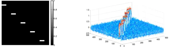
Figure 1: (left) Synthetic500×500binary dataD; (right) mesh view of noisy dataA0.1.
computations significantly using our sparse sketch. Finally, our results are comparable (if not better) than those of Achlioptas et al. (2013b) despite using significantly less information about the data.
1.4 A Motivating Example for Hybrid Sampling
The main motivation for introducing the idea of hybrid-(`1, `2)sampling comes from achieving a
tighter bound onsusing a simple and intuitive probability distribution on elements ofA. For this, we observe certain good properties of both`1 and`2 sampling for sparsification of noisy data (in
practice, we experience data that are noisy, and it is perhaps impossible to separate “true” data from noise). We illustrate the behavior of`1and`2 sampling on noisy data using the following synthetic
example. We construct a500×500binary dataD(FIGURE 1), and then perturb it by a random Gaussian matrixNwhose elementsNij follow Gaussian distribution with mean zero and standard
deviation0.1. We denote this perturbed data matrix byA0.1. First, we note that`1and`2sampling
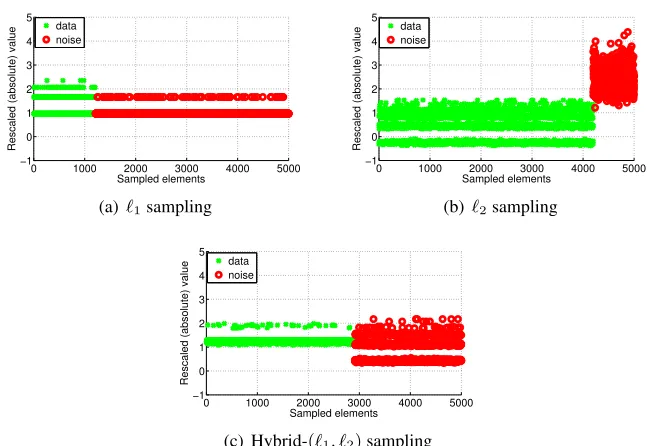
workidenticallyon binary dataD. However, FIGURE 2 depicts the change in behavior of`1and
`2 sampling to sparsify A0.1. Data elements and noise in A0.1 are the elements with non-zero
and zero values in D, respectively. We sample s = 5000indices in i.i.d. trials according to `1
and`2 probabilities separately to produce sparse sketchA˜. FIGURE 2 shows that elements ofA˜,
produced by`1 sampling, have controlled variance but most of them are noise. On the other hand,
`2 sampling is biased towards data elements, although small number of sampled noisy elements
create large variance due to rescaling. Such large magnitude noisy elements become outliers in
˜
A; consequently, PCA on A˜ becomes a poor approximation to the true PCA of A. Our
hybrid-(`1, `2)sampling benefits from this bias of`2towards data elements to sample large number of true
data. Additionally, the regularization property of`1component prevents noisy elements to become
outliers inA˜ helping us to achieve near-PCA reconstruction.
We parameterize our distribution using the variableα∈(0,1]that controls the balance between `2 sampling and`1 regularization. One can view α as a regularization parameter. We derive an
expression to computeα∗, the optimalα, corresponding to the smallest sample size that we need to achieve an accuracyin (1). Whenα = 1we reproduce the result of Achlioptas et al. (2013a). However, α∗ may be smaller than 1, and the bound on sample size, usingα∗, is guaranteed to be tighter than that of Achlioptas et al. (2013a) and`2.
2. Main Results
0 1000 2000 3000 4000 5000 −1 0 1 2 3 4 5
Rescaled (absolute) value
Sampled elements data
noise
(a)`1sampling
0 1000 2000 3000 4000 5000
−1 0 1 2 3 4 5 Sampled elements
Rescaled (absolute) value
data noise
(b)`2sampling
0 1000 2000 3000 4000 5000
−1 0 1 2 3 4 5 Sampled elements
Rescaled (absolute) value
data noise
(c) Hybrid-(`1, `2)sampling
Figure 2: Elements of sparse sketchA˜ produced fromA0.1by (a)`1, (b)`2, and (c) hybrid-(`1, `2),
α = 0.7 sampling. In each plot, x-axis is the number of sampled indicess = 5000, including both data and noise. y-axis plots the rescaled absolute values (inlnscale) of
˜
Acorresponding to the sampled indices. `1sampling produces elements with controlled
variance but it mostly samples noise, whereas`2samples a lot of data although producing
large variance of rescaled elements. Hybrid-(`1, `2) sampling uses `1 as a regularizer
while sampling fairly large number of data that helps to preserve the spectral structure of original data. Data and noisy elements are shown as clusters for better visualization.
of elements fromAas follows. We can expressAas a sum of matrices each having at most one non-zero element.
A=
m,n
X
i,j=1
AijeieTj, ∀(i, j)∈[m]×[n] (4)
We sample (in i.i.d. trials) some of the terms in (4) according to some probability distribution
{pij}m,ni,j=1defined over the elements ofAto form a (weighted) partial sum that represents our sparse
sketchA˜ ofA. More formally, we define the following sampling operatorSΩ :Rm×n→Rm×nin (5) that extracts some of the terms from (4). LetΩ⊂[m]×[n]be a multi-set of sampled indices
(it, jt), fort= 1, ..., s. Then,
˜
A=SΩ(A) =
1
s
s
X
t=1
Aitjt
pitjt eite
T
jt, (it, jt)∈Ω (5)
according topij’s as in equation (3). In order to boundkA−A˜k2we first expressA−A˜ as a sum of
zero-mean, independent, random matrices, and then use the following matrix-Bernstein inequality in Lemma 1 (due to Recht 2011) that bounds the deviation of spectral norms of such matrices.
Lemma 1 [Theorem 3.2 of Recht 2011] LetM1,M2, ...,Ms be independent, zero-mean random matrices inRm×n. Supposemaxt∈[s]
kE(MtMTt)k2,kE(MTtMt)k2 ≤ρ2,andkMtk2 ≤γ for
allt∈[s]. Then, for any > 0, 1s Ps
t=1Mt
2 ≤holds, subject to a failure probability at most
(m+n)exp −
s2/2
ρ2+γ/3
.
A popular construction ofMt∈Rm×n,t∈[s], in Lemma 1 isMt=
Aitjt
pitjt eite T
jt−Aforpitjt 6= 0.
Clearly, 1sPs
t=1Mt = ˜A−A.We can see that ρ2 andγ of Lemma 1 are now dependent onpij
(Lemmas 8 and 9), i.e., different choices ofpij lead to different bounds onρ2 andγ. Now, upper
bounding the failure probability in Lemma 1 by δ > 0, we can express the sample sizes as a function of the key quantitiesρ2andγ, and consequently as a function ofpij:
s≥ 2
2 ·(ρ
2+γ/3)·ln((m+n)/δ).
Since our choice ofpij in (3) is a function of distribution parameterα, we essentially parameterize
ρ2 andγ byα, and expresssas a function ofα. Let us definef(α)as follows.
f(α) =ρ2(α) +γ(α)kAk2/3,
where
γ(α) = max
i,j:
Aij6=0
(
kAk1
α+ (1−α)kAk1·|Aij| kAk2
F
)
+kAk2, (6)
ρ2(α) = maxnmax
i n
X
j=1
ξij(α),max j
m
X
i=1
ξij(α)
o
−σmin2 , (7)
ξij(α) = kAk2F/
α· kAk2
F
|Aij| · kAk1
+ (1−α)
,Aij 6= 0, (8)
σminis the smallest singular value ofA. Such parameterization gives us a flexibility to express the
sample size as a function ofα:s(α) ∝f(α). Naturally, we want to findα ∈(0,1]that results in the smallests(α). The optimalαmay be less than 1, and settingα = 1(in which case equation 3 coincides with`1probabilities of Achlioptas et al. 2013a) may not produce the smallests.
We can see thatγ(α)preventsf(α)from blowing up (in case of sampling a tiny element ofA) by settingαaway from 0 (this is a regularization step). Thus,ρ2(α)becomes the dominating term
inf(α)asγ(α)is multiplied by a small constant. We take a closer look atξij(α)as it is the key
quantity inρ2(α) which is approximately the larger of the largest row sum or the largest column
sum ofξij(α). While minimizingf(α),αmaintains a trade-off between the two terms α
·kAk2
F |Aij|·kAk1
and(1−α)such that the maximum row sum or column sum ofξij(α)gets smaller. Along rowi
or columnj, for smaller|Aij|, we typically have|Aij| · kAk1 <kAk2F, and consequentlyα→ 1
reduces ρ2(α). On the other hand, for larger |Aij|we have |Aij| · kAk1 > kAk2F andα away
Algorithm 1Element-wise Matrix Sparsification
1: Input:A∈Rm×n, accuracy >0.
2: Setsas in eq. (11).
3: For t = 1. . . s (i.i.d. trials with replacement)randomly sample pairs of indices (it, jt) ∈
[m]×[n]withP[(it, jt) = (i, j)] = pij, wherepij are as in (3), usingαas in (10).
4: Output:SΩ(A) = 1sPst=1
Aitjt
pitjt eite T jt.
depending on the structure of the data. Note that forα= 1(as in Achlioptas et al. 2013a) we have
ξij(α) =|Aij| · kAk1. Therefore, for larger|Aij|(true data points), maximum row sum or column
sum ofξij(α)lose the benefit of the delicate role played byα < 1to reduce those quantities, and
they become larger than that forα <1. Thus, parameterization and optimization withαgives us a strictly smaller sample size than that of`1or`2sampling for the problem in (1).
Our main algorithm Algorithm 1 leads us to the following theorem.
Theorem 2 LetA ∈ Rm×n and let > 0 be an accuracy parameter. Let S
Ω be the sampling operator defined in (5), and assume that the multi-setΩis generated using sampling probabilities
{pij}m,ni,j=1as in (3). Then, with probability at least1−δ,kSΩ(A)−Ak2≤kAk2,if
s≥ 2
(kAk2)2
·f(α)·ln((m+n)/δ). (9)
Furthermore, we can findα∗(optimalαcorresponding to the smallests) by solving (10):
α∗ = min
α∈(0,1]f(α), (10)
and the corresponding optimal sample size is
s∗ = 2
(kAk2)2 ·f(α
∗)·ln((m+n)/δ). (11)
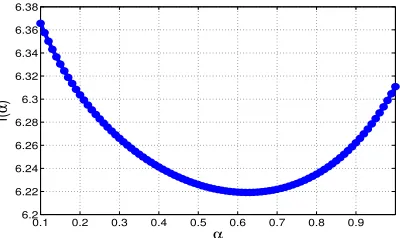
For a given matrix A, we can easily computeρ2(α) andγ(α)for various values ofα. Given an accuracyand failure probabilityδ, we can computeα∗corresponding to the tightest bound on s. Note that, forα= 1we reproduce the results of Achlioptas et al. (2013a) (which was expressed using various matrix metrics). However,α∗ may be smaller than 1, and is guaranteed to produce tighterscomparing to extreme choices ofα (e.g. α = 1for`1). We illustrate this in FIGURE 3.
We give a proof of Theorem 2 in APPENDIX A.
2.1 Approximation of PCA via Element Sampling
The top-k principal components of centered data A ∈ Rm×n (m data points in n dimensions), denoted byVk∈Rn×k, can be formulated as the solution to the variance maximization problem:
Vk= argmax
V∈Rn×k,VTV=I
trace(VTATAV). (12)
The maximum variance achievable usingVk, denoted byOP Tk, is the sum of squares of the top-k
0.1 0.2 0.3 0.4 0.5 0.6 0.7 0.8 0.9 6.2
6.22 6.24 6.26 6.28 6.3 6.32 6.34 6.36 6.38
α
f(
α
)
Figure 3: Plot off(α)in eqn. (10) for dataA0.1. We use= 0.05andδ= 0.1.x-axis plotsαand
y-axis is in log scale.
Algorithm 2Approximation of PCA from Data Samples
1: Input:Centered dataA∈Rm×n, sparsity parameters >0, and rank parameterk.
2: Produce sparse unbiased sketchA˜ fromA, insi.i.d. trials using Algorithm 11.
3: Perform rank truncated SVD on matrixA˜, i.e.,[ ˜Uk,D˜k,V˜k]= SVD(A˜,k).
4: Output:V˜k(columns ofV˜kare the ordered principal components).
Here we discuss a provable algorithm (Algorithm 2) to approximate PCA by applying element-wise sampling. We produce a sparse unbiased estimator A˜ of centered data A by sampling s elements in i.i.d. trials according to our hybrid-(`1, `2)distribution in (3). We use thisA˜ instead of
Ain (12) to compute the new optimal solutionV˜k
˜
Vk= argmax
V∈Rn×k,VTV=I
trace(VTA˜TAV˜ ). (13)
The computation of rank-truncated SVD on sparse data requires fewer floating point operations (therefore can be fast), and we consider the right singular vectors V˜k of A˜ as the approximate
principal components ofA. Naturally, more samples produce better approximation. However, this reduces sparsity, consequently we may lose the speed advantage. Theorem 3 shows the quality of approximation of principal components produced by Algorithm 2.
Theorem 3 LetA∈Rm×nbe a given matrix, andA˜ be a sparse sketch produced by Algorithm 1. LetV˜kbe the PCA’s ofA˜ computed in step 3 of Algorithm 2. Then
1) kA−AV˜kV˜kTk2F ≤ kA−Akk2F + 4kAkk2F · kA−A˜k2/σk(A),
2) kAk−A˜kkF ≤
√
8k·(kA−Akk2+kA−A˜k2),
3) kA−A˜kkF ≤ kA−AkkF +
√
8k·(kA−Akk2+kA−A˜k2).
1. Here we avoid computingkAk2directly and instead upper bound it bykAkFinγ(α)in Lemma 8. In (10)ρ2(α)is the dominating term (we ignoreσminas it is typically very small) andγ(α)is multiplied by a small constant; thus
The first inequality of Theorem 3 bounds the approximation of projected data onto the space spanned by topkapproximate principal components. The second and third inequalities measure the quality ofA˜kas a surrogate forAkand the quality of projection of sparsified data onto approximate
principal components, respectively. The proofs of first two inequalities of Theorem 3 follow from Theorem 5 and Theorem 8 of Achlioptas and McSherry (2001), respectively. The last inequality follows from the triangle inequality. The last two inequalities above are particularly useful in cases whereAis inherently low-rank and we choose an appropriatekfor whichkA−Akk2is small.
2.2 Approximating Sparse PCA from Incomplete Data
PCA constructs a low dimensional subspace of the data such that projection of the data onto this subspace preserves as much information as possible. However a shortcoming of PCA is the in-terpretation of the principal components (or factors) as they can be linear combinations of allthe original variables. In many cases the original variables have direct physical significance (e.g. genes in biological applications or assets in financial applications). In such cases it is desirable to have factors which have loadings on only a small number of the original variables. These interpretable factors are sparse principal components (SPCA). To derive sparse principal components, we add a sparsity constraint to the optimization problem (see equation 14): every column ofVshould have at mostrnon-zero entries (ris an input parameter),
Sk= argmax
V∈Rn×k,VTV=I,kV(i)k 0≤r
trace(VTATAV). (14)
The sparse PCA problem is not only NP-hard, but also inapproximable (Magdon-Ismail 2017). There are many heuristics for obtaining sparse factors (Cadima and Jolliffe, 1995; Trendafilov et al., 2003; Zou et al., 2006; d’Aspremont et al., 2007, 2008; Moghaddam et al., 2006; Shen and Huang, 2008) including some approximation algorithms with provable guarantees Asteris et al. (2014). The existing research typically addresses the task of getting just the top principal component (k = 1) (some exceptions are Ma 2013; Cai et al. 2013; Wang et al. 2014; Lei and Vu 2015). While the sparse PCA problem is hard and interesting, it isnotthe focus of this work.
We address the question: What if we do not knowA, but only have a sparse sampling of some of the entries inA(incomplete data)? The sparse sampling is used to construct asketchofA, denoted
˜
A. There is not much else to do but solve the sparse PCA problem with the sketchA˜ instead of the full dataAto getS˜k,
˜
Sk= argmax
V∈Rn×k,VTV=I,kV(i)k0≤r
trace(VTA˜TAV˜ ). (15)
We study how S˜k performs as an approximation to Sk with respective to the objective that we
are trying to optimize, namely trace(STATAS)— the quality of approximation is measured with respect to the trueA. We show that the quality of approximation is controlled by how wellA˜TA˜
approximates ATAas measured by the spectral norm of the deviation ATA−A˜TA˜. This is a general result that does not rely on how one constructs the sketchA˜.
Lemma 4 (Sparse PCA from a Sketch) Let Sk be a solution to the sparse PCA problem that solves (14), and S˜k a solution to the sparse PCA problem for the sketch A˜ which solves (15). Then,
Lemma 4 says that if we can closely approximateAwithA˜, then we can compute, fromA˜, sparse components which capture almost as much variance as the optimal sparse components computed from the full dataA. We prove that Lemma 4 follows as a corollary of a more general result given in Theorem 10.
In our setting, the sketch A˜ is computed from a sparse sampling of the data elements in A
(incomplete data). We use probabilities of the form in (3) to determine which elements to sample and how to form the sketch such that the errorkATA−A˜TA˜k2 is small. We can simplify this
quantity in terms ofkA−A˜k2as follows. Let∆ =A−A˜.
kATA−A˜TA˜k2=kAT∆ + ∆TA−∆T∆k2≤2kAk2k∆k2+k∆k2
2. (16)
We combine the bound onkA−A˜k2 for given accuracy/k from Theorem 2 with Lemma 4 to
derivekkATA−A˜TA˜k2 ≤(2 +/k)kAk2
2with a sample sizes=k2·s∗wheres∗as in (11).
However, we simplify this bound for a better interpretation ofsin terms matrix dimensionsmand nand stable rankk˜=kAk2
F/kAk22. Note thatkAk1≤
√
mnkAkF from Cauchy-Schwartz. Then,
γ(α)/kAk2≤1 +kAk1/(αkAk2)≤1 +
p
mnk/α˜ = ˆγ. (17)
Also, from|Aij| ≤ kAk2,ρ2(α)in (7) can be simplified as
ξij(α) ≤ kAk2F
α˜kkAk2/kAk1+ (1−α)
−1
, (18)
ρ2(α)/kAk2
2 ≤ max{m, n}˜k
αk˜kAk2/kAk1+ (1−α)−1= ˆρ2. (19)
Using the above relaxations we have the following theorem on sample size complexity.
Theorem 5 (Sampling Complexity for Sparse PCA) Samplesdata-elements fromA∈Rm×nto form the sparse sketchA˜ using Algorithm 1. LetSkbe a solution to the sparse PCA problem that solves (14), and letS˜k, which solves (15), be a solution to the sparse PCA problem for the sketchA˜ formed from thessampled data elements. Suppose the number of samplesssatisfies
s≥2k2−2( ˆρ2+γ/ˆ (3k)) log((m+n)/δ),
(ρˆ2andγˆare dimensionless quantities that depend only onA). Then, with probability at least1−δ
trace(˜SkTATAS˜k)≥trace(SkTATASk)−2(2 +/k)kAk22.
The dependence ofρˆ2 andγˆonAare given in (17) and (19), respectively. Roughly speaking, we can ignore the term withˆγ since it is multiplied by/k, and we haveρˆ2=O(˜kmax{m, n}). To paraphrase Theorem 5, when the stable rankk˜is a small constant, withO(k2max{m, n})samples, one can recover almost as good sparse principal components as with all data (a possible price being a small fraction of the optimal variance, sinceOP Tk≥ kAk22). As far as we know, the only prior
2.2.1 SPARSESKETCH USINGGREEDYTHRESHOLD
We also give an application of Lemma 4 to run sparse PCA after “denoising” the data using a greedy thresholding algorithm that sets the small elements to zero (see Theorem 6). Such denoising is appropriate when the observed matrix has been element-wise perturbed by small noise, and the uncontaminated data matrix is sparse and contains large elements. We show that if an appropriate fraction of the (noisy) data is set to zero, one can still recover sparse principal components. This gives a principled approach to regularizing sparse PCA in the presence of small noise when the data is sparse.
We give the simplest scenario of incomplete data where Lemma 4 gives some reassurance that one can compute good sparse principal components. Suppose the smallest data elements have been set to zero. This can happen, for example, if only the largest elements are measured, or in a noisy setting if the small elements are treated as noise and set to zero. So
˜
Aij =
(
Aij |Aij| ≥δ,
0 |Aij|< δ.
Recall˜k=kAk2
F/kAk22(stable rank ofA), and definekAδk2F =
P
|Aij|<δA 2
ij. Let∆ =A−A˜.
By construction,k∆k2
F =kAδk2F andkATA−A˜TA˜k2 ≤2kAk2k∆k2+k∆k22 from (16).
Sup-pose the zeroing of elements only loses a fraction of the energy inA, i.e. δ is selected so that
kAδk2F ≤2kAk2F/˜k; that is an/k˜fraction of the total variance inAhas been lost in the
unmea-sured (or zero) data. Thenk∆k2≤ k∆kF ≤kAkF/pk˜=kAk2.
Theorem 6 Suppose thatA˜ is created fromAby zeroing all elements that are less thanδ, andδ
is such that the truncated norm satisfieskAδk22≤2kAk2F/˜k. Then the sparse PCA solutionV˜∗ satisfies
trace( ˜V∗TAAV˜∗)≥trace(V∗TAATV∗)−2kkAk22(2 +).
Theorem 6 shows that it is possible to recover sparse PCA after setting small elements to zero. This is appropriate when most of the elements in A are small noise and a few of the elements in A
contain large data elements. For example if the data consists of sparseO(√nm)large elements (of magnitude, say 1) and manynm−O(√nm)small elements whose magnitude iso(1/√nm)(high signal-to-noise setting), then kAδk22/kAk22 →0and with just a sparse sampling of the O(
√
nm)
large elements (very incomplete data), we recover near optimal sparse PCA.
Not only do our algorithms preserve the quality of the sparse principal components, but iterative algorithms for sparse PCA, whose running time is proportional to the number of non-zero entries in the input matrix, benefit from the sparsity ofA˜. Our experiments show about five-fold speed gains while producing near-comparable sparse components using less than 10% of the data.
2.3 One-pass Hybrid-(`1, `2)Sampling
Here we discuss the implementation of hybrid-(`1, `2)sampling in one pass over the input
ma-trixAusing O(s)memory, e.g., a streaming model. Here we propose an algorithm, Algorithm 3, to implement a one-pass version of the hybrid samplingwithout a priori knowledge of the regular-ization parameterα.
We use SELECT-salgorithm (Algorithm 5 in APPENDIX F) to implement one-pass`1 and`2
Algorithm 3One-pass hybrid sampling
1: Input:Aij for all(i, j)∈[m]×[n], arbitrarily ordered, and sample sizes.
2: Apply SELECT-s algorithm (Algorithm 5) using `1 probabilities to sample s independent
indices (it1, jt1) and corresponding values Ait1jt1 to form random multiset S1 of triples
(it1, jt1,Ait1jt1), fort1= 1, ..., s.
3: Apply SELECT-salgorithm using `2 probabilities to samplesindependent indices (it2, jt2)
and corresponding valuesAit2jt2 to form random multisetS2 of triples(it2, jt2,Ait2jt2), for
t2= 1, ..., s.
4: Store kAk2F andkAk1/* these are already computed in SELECT-salgorithms above */
5: /* stream terminates */
6: Set the value ofα∈(0,1](say, using Algorithm 4).
7: Create empty multiset of triplesS.
8: X←0m×n.
9: Fort= 1. . . s
10: Generate a uniform random numberx∈[0,1].
11: ifx≤α,S(t)←S1(t); otherwise,S(t)←S2(t).
12: (it, jt)←S(t,1 : 2).
13: p←α·|S(t,3)kAk |
1 + (1−α)·
|S(t,3)|2 kAk2
F
14: X←X+S(t,3)p·s eite T jt.
15: End
16: Output:random multisetS, and sparse matrixX.
to form independent multisetsS1 andS2. We store kAk2F and kAk1 already computed in steps
2-3. Subsequent steps do not need further access to A. Interestingly, we set α in step 6 when the data stream terminates. Steps 9-15 sampleselements from S1 andS2 using theα in step 6,
and produces a sparse matrix X using the sampled entries in multisetS. Theorem 7 proves that Algorithm 3 indeed samples elements ofAaccording to the hybrid-(`1, `2)probabilities in (3).
Theorem 7 Using the same notations as in Algorithm 3, forα∈(0,1],t= 1, ..., s,
P[S(t) = (i, j,Aij)] =α·
|Aij|
kAk1
+ (1−α)· A
2 ij
kAk2
F
.
See proof in APPENDIX E. Note that, Theorem 7 holds for any arbitraryα ∈ (0,1]in line 7 of Algorithm 3, i.e., Algorithm 4 is not essential for correctness of Theorem 7. We only needαto be independent of the elements ofS1andS2. However, we can use Algorithm 4 to get a good estimate
ofα∗ (SECTION 2.3.1). In this case, we need additional independent samples fromA to ‘learn’ the parameterα∗.
2.3.1 ESTIMATE OFα∗FROMSAMPLES
Here we discuss Algorithm 4, to estimateα∗ from samples ofAand few other quantities, such as,
kAkF,kAk1, andAmin, whereAminis defined as
Amin= min i,j:
Aij6=0
Algorithm 4Estimatingα∗from Samples
1: Input: Ω, the set of triples {(i, j,Aij)} where eachAij is sampled with probabilitypij (say
pij =|Aij|/kAk1), accuracyε,Amin,kAk2F,kAk1, and matrix dimensionsmandn.
2: Computeγ˜(α)as in equation (20) andξ˜ij(α)as in equation (21), for a givenα.
3: Output:α˜in equation (23).
LetΩbe a set of sampled triples{(i, j,Aij)}where eachAij is sampled with probabilitypij (e.g.,
pij =|Aij|/kAk1). Let us define, for a fixedα,
˜
γ(α) = max
i,j:
Aij6=0
(
kAk1
α+ (1−α)kAk1·|Aij| kAk2
F
)
+kAkF = kAk1
α+ (1−α)kAk1
kAk2
F
·Amin
+kAkF. (20)
Note that,˜γ(α)can be computed using only one pass over the data. Further, we define the following random variable (parameterized byα)
˜
ξij(α) =
kAk2
F α·kAk2
F
|Aij|·kAk1 + (1−α)
·δij, (21)
whereδij is an indicator function defined asδij := I((i, j,Aij)∈ Ω). Note that,δij = 1w.p. pij,
and0otherwise. For a given columnj, we define the following random variableY˜j(α):
˜
Yj(α) = m
X
i=1
˜
ξij(α).
Similarly, for a given rowi, we defineY˜i(α) =Pnj=1ξ˜ij(α). Finally, we define
˜
ρ2(α) = max{max
j
˜
Yj(α),max i
˜
Yi(α)}. (22)
Using the above quantities we solve the optimization problem in (23) and use the solution as an estimate forα∗.
˜
α: min
α∈(0,1] ρ˜
2(α) + ˜γ(α)ε/3. (23)
Note that, γ˜(α) in equation (20) closely approximates γ(α) in equation (6), where the error of approximation iskAkF− kAk2. This error becomes small in equation (23) asγ˜(α)is multiplied by a small quantityε/3. Next we analyze how wellξ˜ij(α)approximatesξij(α)using a simplified data
model. For this we assume|Aij| ∈ {L, ,0}, whereL >0, and letsLandsbe the number
of elements with magnitudesLand, respectively. Also, let the minimum singular valueσmin≈0.
For(i, j,Aij)∈Ωand|Aij|=(which is unlikely),|Aij| · kAk1 kAk2F; consequentlyξ˜ij(α)
is small and does not contribute much toY˜j(α)(orY˜i(α)). On the other hand, for(i, j,Aij) ∈Ω
and|Aij|=L(which is very likely),|Aij| · kAk1 kAk2F, and consequentlyξ˜ij(α)contributes
significantly toY˜j(α)(orY˜i(α)). So, if we samplesLnumber of such large elementsρ˜2(α)is close
3. Experiments
We perform various element-wise sampling on synthetic and real data to show how well the sparse sketches preserve the structure of the original data, in spectral norm. Also, we show results on the quality and computation time of the principal components and sparse principal components derived from sparse sketches.
3.1 Algorithms for Sparse Sketches
Algorithm 1 is our prototypical algorithm to produce (unbiased) sparse sketchesA˜ from a given ma-trix via various sampling methods. We construct our sparse sketch using our optimal hybrid-(`1, `2)
probabilities, and compare its quality with other sketches produced via `1 and `2 sampling. We
borrow same definitions from (Achlioptas et al. 2013a) for comparing our results with`1sampling.
nd(A) := kAk
2 1
kAk2
F
, rs0(A) :=
maxikA(i)k0
kAk0/m , rs1(A) :=
maxikA(i)k1
kAk1/m ,
where nd is numeric density and rs is row density skewness. Achlioptas et al. (2013a) argues that`1
outperforms`2sampling when rs0 >rs1. We compute the theoretical optimal mixing parameterα∗
by solving (10) for various datasets2, and compare thisα∗with the theoretical condition derived by Achlioptas et al. (2013a). Further, we verify the accuracy ofα∗by measuringE =kA−A˜k2/kAk2
for distributions corresponding to variousα, for a given sample size s3. We expectE to be the smallest forα≈α∗rather thanα = 1(`1) orα≈0(`2).
3.2 Algorithms for PCA from Sparse Sketches
We first compare three algorithms for computing PCA of the centered dataA. Let the actual PCA of the original data beA. We use Algorithm 2 to compute approximate PCA from random samples via our optimal hybrid-(`1, `2) sampling. Let us denote this approximate PCA byH. Also, we
compute PCA of a Gaussian random projection of the original data to compare its quality withH. LetAG=GA∈Rr×n, whereA∈Rm×nis the original data, andGis ar×mstandard Gaussian matrix. Let the PCA of this random projectionAGbeG. The quality of various PCA is determined
by measuring how much variance of the data they can capture (as in equation 12). For this, letσk,
σh, andσg denote the variance preserved byA,H, andG, respectively. Note that,AandGrequire
access to the full data, whileHis computed from only few samples ofA. Also, we compare the computation time (in milliseconds)ta,th, andtGforA,H, andG, respectively.
Finally, we compare the quality of our optimal hybrid sampling with `1 sampling and
Bern-stein sampling (Achlioptas et al. 2013b) by quantifying the variance,σ`1 andσb, preserved by the
corresponding sparse sketches.
3.3 Algorithms for Approximate Sparse PCA from Sketches
We show the experimental results for sparse PCA from a sketch using several real data matrices. As we mentioned, sparse PCA is NP-Hard, and so we use heuristics. These heuristics are discussed next, followed by the data, the experimental design and finally the results.
2. we findα∗from the plot off(α)forα∈[0.1,1].
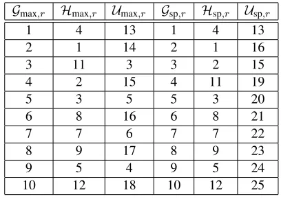
Let G (ground truth) denote the algorithm which computes the principal components (which may not be sparse) of the full data matrix A; the optimal variance is OP Tk. We consider six
heuristics for getting sparse principal components.
Gmax,r Therlargest-magnitude entries in each principal component generated byG.
Gsp,r r-sparse components using theSpasmtoolbox of Sjstrand et al. (2012) withA.
Hmax,r Therlargest entries of the principal components for the(`1, `2)-sampled sketchA˜.
Hsp,r r-sparse components usingSpasmwith the(`1, `2)-sampled sketchA˜.
Umax,r Therlargest entries of the principal components for theuniformlysampled sketchA˜.
Usp,r r-sparse components usingSpasmwith the uniformly sampled sketchA˜.
Output of an algorithmZis sparse principal componentsV, and we consider the metricf(Z) =
trace(VTATAV), whereAis the original centered data. We consider the following statistics. f(Gmax,r)
f(Gsp,r)
Relative loss of greedy thresholding versusSpasm, illustrating the value of a good sparse PCA algorithm. Our sketch based algorithmsdo notaddress this loss.
f(Hmax/sp,r)
f(Gmax/sp,r) Relative loss of using the(`1, `2)-sketchA˜ instead of complete data A. A ratio
close to 1 is desired. f(Umax/sp,r)
f(Gmax/sp,r) Relative loss of using the uniform sketchA˜ instead of complete dataA. A
bench-mark to highlight the value of a good sketch.
We also report the computation time for the algorithms. We show results to confirm that sparse PCA algorithms using the(`1, `2)-sketch are nearly comparable to those same algorithms on the
complete data; and, gain in computation time from sparse sketch is proportional to the sparsity. Also, we evaluate the quality of Algorithm 4 to estimateα∗ from a small number of samples from various data.
3.4 Other Sketching Probabilities
We considerpij proportional to the sum of row and columnleverage scoresofA(Chen et al. 2014)
to produce sparse sketchA˜ using Algorithm 1. LetAbe anm×nmatrix of rank%, and its SVD is given byA =UΣVT, whereUandVcontains% orthonormal left and right singular vectors, respectively, andΣis the diagonal matrix of singular values. We define leverage scores as follows (as in Mahoney and Drineas 2009)
(row leverage) µi = kU(i)k22, ∀i∈[m]
(column leverage) νj = kV(j)k22, ∀j∈[n]
and element-wise leverage score (similar to Chen et al. 2014)
plev=
1 2
µi+νj
(m+n)% +
1
2mn, i∈[m], j ∈[n].
Note thatplevis a probability distribution on the elements ofA. At a high level, the leverage scores
of an element(i, j)is proportional to the squared norms of thei-th row of the left singular matrix and thej-th row of the right singular matrix. The constant term inplev prevents the rescaled values
from blowing up in case of sampling an element with tiny leverage score. Such leverage score sampling is distinct from uniform sampling only forlow-rankmatrices orlow-rank approximations
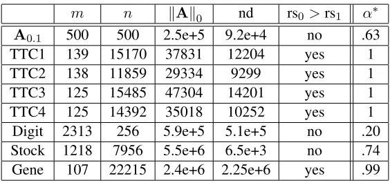
m n kAk0 nd rs0>rs1 α∗
A0.1 500 500 2.5e+5 9.2e+4 no .63
TTC1 139 15170 37831 12204 yes 1
TTC2 138 11859 29334 9299 yes 1
TTC3 125 15485 47304 14201 yes 1
TTC4 125 14392 35018 10252 yes 1
Digit 2313 256 5.9e+5 5.1e+5 no .20
Stock 1218 7956 5.5e+6 6.5e+3 no .74
Gene 107 22215 2.4e+6 2.25e+6 yes .99
Table 1: α∗ for variousm×ndata sets (=.05is the desired relative-error accuracy). rs0 >rs1
implies`1is better than`2(Achlioptas et al. 2013a), and we reproduce this (α∗= 1). But,
for rs0 ≤rs1,α∗ <1and our hybrid sampling is strictly better than both`1and`2.
3.5 Description of Data
Synthetic Data: A0.1as described in SECTION 1.4 (FIGURE 1).
TechTC Datasets (TTC):(Gabrilovich and Markovitch 2004) These datasets are bag-of-words fea-tures for document-term data describing two topics (ids). We choose four such datasets. Rows represent documents and columns are the words. We preprocessed the data by removing all the words of length four or smaller, and then divide each row by its Frobenius norm.
Digit Data: (Hull 1994) A data set of three handwritten digits: six (664 samples), nine (644 sam-ples), and one (1005 samples). Pixels are treated as features, and pixel values are normalized in [-1,1]. Each16×16digit image is encoded to form a row in the data matrix (2313 rows and 256 columns).
Stock Data(S&P): We use a temporal data containing 1218 stocks (rows) collected between 1983 and 2011. This temporal data set has with 7056 snapshots (columns) of prices.
Gene Expression Data: We use GSE10072 gene expression data for lung cancer from NCBI Gene Expression Omnibus database. There are 107 samples (58 lung tumor cases and 49 normal lung controls) forming the rows of the matrix, with 22,215 probes (features) from GPL96 platform annotation table.
3.6 Results
All the random results are based on mean of several independent trials (small variance observed).
3.6.1 QUALITY OFSPARSESKETCH
Table 1 summarizesα∗ for various data sets. Achlioptas et al. (2013a) argued that, for rs0 > rs1,
`1 sampling is better than `2 (even with truncation). Our results on α∗ in Table 1 reproduce this
condition (α∗ = 1 implies `1). Moreover, our method can derive the right blend of `1 and `2
s/(k(m+n)) αˆ
A0.1,k= 5 2 0.7
3 0.7
Digit,k= 3 3 0.3
5 0.3
Stock,k= 1 2 0.7
3 0.7
Table 2: αˆ corresponding to the minimum relative error kA−A˜k2/kAk2, for a fixed budget of
samples sizes. αˆ ≈α∗ in Table 1, indicating that our optimal hybrid sampling produces strictly better sparse sketch than both`1and`2.k≈ kAk2F/kAk22(stable rank).
Also, we note the value ofα4for the minimum relative error kA−A˜k2
kAk2 , for a fixed sample size
sin Table 2. Table 2 shows that the quality of the sparse sketch produced by our optimal hybrid sampling is strictly better than that of both`1and`2.
•Comparison with`2-with-truncation: We also compare our optimal hybrid sampling with`2
sampling with truncation. We use two predetermined truncation parameters,ε= 0.1andε= 0.01. First, `2 sampling without truncation turns out to produce the worst quality sparse sketches for
all datasets. For real datasets, hybrid-(`1, `2) sampling using α∗ outperforms `2 with truncation
ε= 0.1andε= 0.01. ForA0.1,`2withε= 0.01appears to produceA˜ that is as bad as`2without
truncation. However,`2withε= 0.1shows better quality than optimal hybrid sampling (forA0.1
only) as thisεfilters out the noisy elements. We should point out that we know a goodεforA0.1
as we control the noise in this case. However, in reality, we have no control over the noise, and choosing the rightεwith no prior knowledge of the data, is an improbable outcome.
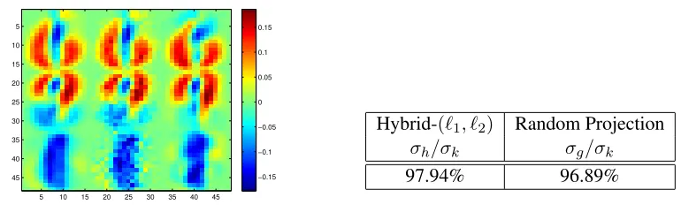
3.6.2 QUALITY OFPCAFROM SPARSE SKETCHES
We investigate the quality of Algorithm 2 for Digit data andA0.1. We setr = 30kfor the random
projection matrixAG to achieve a comparable runtime ofG with H(k is 3 and 5 for Digit and
A0.1, respectively). FIGURE 4 shows thatHhas better quality thanGfor Digit data. Also, Table 3
lists the gain in computation time for Algorithm 2 due to sparsification (using hybrid sampling with α∗). Finally, our optimal hybrid sampling outperforms`1and Bernstein sampling (Achlioptas et al.
2013b) by preserving more variance of data via PCA (Table 4).
3.6.3 QUALITY OFSPARSEPCA ALGORITHMS
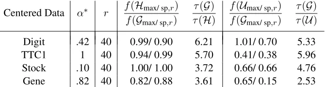
We report results for primarily the top principal component (k= 1) which is the case most consid-ered in the literature. When k >1, our results do not qualitatively change. We note the optimal mixing parameterα∗using Algorithm 1 for various datasets in Table 5.
Handwritten Digits.We sample approximately7%of the elements from the centered data using
(`1, `2)-sampling, as well as uniform sampling. The quality of solution for small r is shown in
Table 5, including the running time τ. For this data, f(Gmax,r)/f(Gsp,r)≈0.23 (r = 10), so it
is important to use a good sparse PCA algorithm. We see from Table 5 that the (`1, `2)-sketch
5 10 15 20 25 30 35 40 45 5
10
15
20
25
30
35
40
45 −0.15
−0.1 −0.05 0 0.05 0.1 0.15
Hybrid-(`1, `2) Random Projection
σh/σk σg/σk
97.94% 96.89%
Figure 4: [Digit data] Approximation quality of PCA (Algorithm 2) from samples of data. (Left) Visualization of principal components as16×16image. Principal components are or-dered from the top row to the bottom. First column of PCA’s are exact (A). Second column of PCA’s (H) are computed on sparse sketch with 7%non-zeros of all the ele-ments via hybrid sampling using optimalα. Third column of PCA’s (G) are computed onAG. (Right) Variance preserved by PCA algorithms. Hybrid sampling based PCA,
despite using less information, is better than PCA of random projection.
Sparsified Digit SparsifiedA0.1
# non-zeros 7% 6%
ta/th/tG 151/30/36 73/18/36
Table 3: Computational gain of Algorithm 2 comparing to exact PCA. We report the computation time of MATLAB function ‘svds(A,k)’ for actual dataA(ta), sparsified dataA˜ (th), and
random projection dataAG(tG). We use only 7% and 6% of all the elements of Digit data
andA0.1, respectively, to construct respective sparse sketches.k= 3for Digit andk= 5
forA0.1.
significantly outperforms the uniform sketch. A more extensive comparison of recovered variance is given in FIGURE 6(a). We also observe a speed-up of a factor of about 6 for the(`1, `2)-sketch.
We point out that the uniform sketch is reasonable for the digits data because most data elements are close to either+1or−1, since the pixels are either black or white.
We show a visualization of the principal components in FIGURE 5. We observe that the sparse components from the(`1, `2)-sketch are almost identical to that of from the complete data.
TechTC Data. We sample approximately5%of the elements from the centered data using our
(`1, `2)-sampling, as well as uniform sampling. For this data,f(Gmax,r)/f(Gsp,r)≈0.84(r = 10).
We observe a very significant quality difference between the (`1, `2)-sketch and uniform sketch.
A more extensive comparison of recovered variance is given in FIGURE 6(b). We also observe a speed-up of a factor of about 6 for the(`1, `2)-sketch. Unlike the digits data which is uniformly near
`1 Bernstein Hybrid-(`1, `2)
σ`1/σk σb/σk σh/σk
Digit (α∗ = 0.42) 98.47 % 98.46 % 98.51% Stock (α∗ = 0.1) 85.09 % 95.61 % 97.07%
Table 4: Variance preserved by PCA of various sparse sketches. Our optimal hybrid sampling out-performs other sampling methods including Bernstein sampling (Achlioptas et al. 2013b). We sample 9%non-zeros from digit data and2%non-zeros from stock data.
Centered Data α∗ r f(Hmax/ sp,r) f(Gmax/ sp,r)
τ(G)
τ(H)
f(Umax/ sp,r)
f(Gmax/ sp,r)
τ(G)
τ(U)
Digit .42 40 0.99/ 0.90 6.21 1.01/ 0.70 5.33 TTC1 1 40 0.94/ 0.99 5.70 0.41/ 0.38 5.96 Stock .10 40 1.00/ 1.00 3.72 0.66/ 0.66 4.76 Gene .82 40 0.82/ 0.88 3.61 0.65/ 0.15 2.53
Table 5: Comparison of sparse principal components from the(`1, `2)-sketch and uniform sketch.
Recall,Gis the ground truth.
As a final comparison, we look at the actual sparse top component with sparsity parameter r= 10. The topic IDs in the TechTC data are 10567=”US: Indiana: Evansville” and 11346=”US: Florida”. The top-10 features (words) in the full PCA on the complete data are shown in Table 6. In Table 7 we show which words appear in the top sparse principal component with sparsityr= 10
using various sparse PCA algorithms. We observe that the sparse PCA from the(`1, `2)-sketch with
only 5% of the data sampled matches quite closely with the same sparse PCA algorithm using the complete data (Gmax/sp,r matchesHmax/sp,r).
Stock Data. We sample about2%of the non-zero elements from the centered data using the
(`1, `2)-sampling, as well as uniform sampling. For this data,f(Gmax,r)/f(Gsp,r)≈0.96(r = 10).
We observe a very significant quality difference between the (`1, `2)-sketch and uniform sketch.
A more extensive comparison of recovered variance is given in FIGURE 6(c). We also observe a speed-up of a factor of about 4 for the(`1, `2)-sketch. Similar to TechTC data this data set is also
“spikey”, so biased sampling toward larger elements significantly outperforms the uniform-sketch. We now look at the actual sparse top component with sparsity parameterr = 10. The top-10 features (stocks) in the full PCA on the complete data are shown in Table 8. In Table 9 we show which stocks appear in the top sparse principal component using various sparse PCA algorithms. We observe that the sparse PCA from the(`1, `2)-sketch with only 2% of the non-zero elements
sam-pled matches quite closely with the same sparse PCA algorithm using the complete data (Gmax/sp,r
matchesHmax/sp,r).
Gene Expression Data. We sample about9%of the elements from the centered data using the
(`1, `2)-sampling, as well as uniform sampling. For this data,f(Gmax,r)/f(Gsp,r)≈0.05(r = 10)
re-(a)r = 100% (b)r= 50% (c)r= 30% (d)r = 10%
Figure 5: [Digits] Visualization of top-3 sparse principal components. In each figure, left panel showsGsp,rand right panel showsHsp,r.ris the maximum number of non-zeros allowed.
20 40 60 80 100
0.6 0.8 1
Sparsity constraint: r (percent) f(Hsp,r)/f(Gsp,r)
f(Usp,r)/f(Gsp,r)
20 40 60 80 100
0.2 0.4 0.6 0.8
Sparsity constraint: r (percent) f(Hsp,r)/f(Gsp,r)
f(Usp,r)/f(Gsp,r)
20 40 60 80 100
0.6 0.8 1
Sparsity constraint: r (percent) f(Hsp,r)/f(Gsp,r)
f(Usp,r)/f(Gsp,r)
20 40 60 80 100
0.2 0.4 0.6 0.8
Sparsity constraint: r (percent) f(Hsp,r)/f(Gsp,r)
f(Usp,r)/f(Gsp,r)
(a) Digit (b) TechTC (c) Stock (d) Gene
Figure 6: Quality of sparse PCA for(`1, `2)-sketch and uniform sketch over an extensive range for
the sparsity constraintr. The variance preserved by the uniform sketch is significantly lower, highlighting the importance of a good sketch.
covered variance is given in FIGURE 6(d). We also observe a speed-up of a factor of about 4 for the(`1, `2)-sketch. Similar to TechTC data this data set is also “spikey”, and consequently biased
sampling toward larger elements significantly outperforms the uniform-sketch.
Also, we look at the actual sparse top component with sparsity parameter r = 10. The top-10 features (probes) in the full PCA on the complete data are shown in Table top-10. In Table 11 we show which probes appear in the top sparse principal component with sparsityr = 10using various sparse PCA algorithms. We observe that the sparse PCA from the(`1, `2)-sketch with only 9% of
the elements sampled matches reasonably with the same sparse PCA algorithm using the complete data (Gmax/sp,r matchesHmax/sp,r).
Finally, we validate the genes corresponding to the top probes in the context of lung can-cer. Table 12 lists the top twelve gene symbols in Table 10. Note that a gene can occur mul-tiple times in principal component as genes can be associated with different probes. Genes like SFTPC, AGER, WIF1, and FABP4 are down-regulated in lung cancer, while SPP1 is up-regulated (see the functional gene grouping: www.sabiosciences.com/rt_pcr_product/HTML/
PAHS-134Z.html). Co-expression analysis on the set of eight genes for Hmax,r andHsp,r
ID Top 10 inGmax,r ID Other words
1 evansville 11 service 2 florida 12 small
3 south 13 frame
4 miami 14 tours
5 indiana 15 faver 6 information 16 transaction
7 beach 17 needs
8 lauderdale 18 commercial 9 estate 19 bullet 10 spacer 20 inlets
21 producer
Table 6: [TechTC] Top ten words in top prin-cipal component of the complete data (the other words are discovered by some of the sparse PCA algorithms).
Gmax,r Hmax,r Umax,r Gsp,r Hsp,r Usp,r
1 1 6 1 1 6
2 2 14 2 2 14
3 3 15 3 3 15
4 4 16 4 4 16
5 5 17 5 5 17
6 7 7 6 7 7
7 6 18 7 8 18
8 8 19 8 6 19
9 11 20 9 12 20
10 12 21 13 11 21
Table 7: [TechTC] Relative ordering of the words (w.r.t. Gmax,r) in the top sparse
principal component with sparsity pa-rameterr= 10.
ID Top 10 inGmax,r ID Other stocks
1 T.2 11 HET.
2 AIG 12 ONE.1
3 C 13 MA
4 UIS 14 XOM
5 NRTLQ 15 PHA.1
6 S.1 16 CL
7 GOOG 17 WY
8 MTLQQ 9 ROK 10 EK
Table 8: [Stock data] Top ten stocks in top prin-cipal component of the complete data (the other stocks are discovered by some of the sparse PCA algorithms).
Gmax,r Hmax,r Umax,r Gsp,r Hsp,r Usp,r
1 1 2 1 1 2
2 2 11 2 2 11
3 3 12 3 3 12
4 4 13 4 4 13
5 5 14 5 5 14
6 6 3 6 7 3
7 7 15 7 6 15
8 9 9 8 8 9
9 8 16 9 9 16
10 11 17 10 11 17
Table 9: [Stock data] Relative ordering of the stocks (w.r.t. Gmax,r) in the top sparse
principal component with sparsity pa-rameterr= 10.
S1). Further, AGER and FAM107A appear in thetop fivehighly discriminative genes in (Hou et al., 2010, Table S3). Additionally, AGER, FCN3, SPP1, and ADH1B appear among the 162 most dif-ferentiating genes across two subtypes of NSCLC and normal lung cancer in (Dracheva et al., 2007, Supplemental Table 1). Such findings show that our method can identify, from incomplete data, important genes for complex diseases like cancer. Also, notice that our sampling-based method is able to identify additional important genes, such as, FCN3 and FAM107A in top ten genes.
ID Top 10 inGmax,r ID Other probes
1 210081 at 11 205866 at 2 214387 x at 12 209074 s at 3 211735 x at 13 205311 at 4 209875 s at 14 216379 x at 5 205982 x at 15 203571 s at 6 215454 x at 16 205174 s at 7 209613 s at 17 204846 at 8 210096 at 18 209116 x at 9 204712 at 19 202834 at 10 203980 at 20 209425 at 21 215356 at 22 221805 at 23 209942 x at 24 218450 at 25 202508 s at
Table 10: [Gene data] Top ten probes in top principal component of the complete data (the other probes are discovered by some of the sparse PCA algo-rithms).
Gmax,r Hmax,r Umax,r Gsp,r Hsp,r Usp,r
1 4 13 1 4 13
2 1 14 2 1 16
3 11 3 3 2 15
4 2 15 4 11 19
5 3 5 5 3 20
6 8 16 6 8 21
7 7 6 7 7 22
8 9 17 8 9 23
9 5 4 9 5 24
10 12 18 10 12 25
Table 11: [Gene data] Relative ordering of the probes (w.r.t. Gmax,r) in the
top sparse principal component with sparsity parameterr = 10.
Gmax,r ν Hmax,r ν Hsp,r ν
SFTPC 4 SFTPC 3 SFTPC 3
AGER 1 SPP1 1 SPP1 1
SPP 1 1 AGER 1 AGER 1 ADH1B 1 FCN3 1 FCN3 1 CYP4B1 1 CYP4B1 1 CYP4B1 1 WIF1 1 ADH1B 1 ADH1B 1 FABP4 1 WIF1 1 WIF1 1 FAM107A 1 FAM107A 1
Table 12: [Gene data] Gene symbols corresponding to top probes in Table 11. One gene can be associated with multiple probes. Hereν is the frequency of occurrence of a gene in top ten probes of their respective principal component.
3.6.4 ESTIMATE OFα∗FROMSAMPLES
20 40 60 80 100 0.85
0.9 0.95
Sparsity constraint: r (percent) f(Hsp,r),α∗= 0.1
f(Hsp,r),α= 1.0
Figure 7: [Stock data] Quality of sketch using suboptimal α to illustrate the importance of the optimal mixing parameterα∗.
Non-zeros sampled Estimatedα∗
Digit,α∗ = 0.42 6 % 0.80
19 % 0.67
Stock,α∗ = 0.1 2 % 0.1
10 % 0.1
Table 13: Estimatedα∗using Algorithm 4 from small number of non-zeros of Digit and Stock data. Most of elements of Digit data are close to either+1or−1, thus requiring more samples to accurately estimateα∗.
3.6.5 OTHERSKETCHINGPROBABILITIES
We compare the quality of sparse sketches produced from low-rank and rank-truncated synthetic and real data using our optimal hybrid sampling withplev.
• Power-law Matrix: First, we construct a500×500low-rankpower-lawmatrix, similar to Chen et al. (2014), as follows: Apow = DXYTD, where, matrices X andY are500×5i.i.d.
GaussianN(0,1)andDis a diagonal matrix with power-law decay,Dii=i−γ,1≤i≤500. The
parameterγcontrols the ‘incoherence’ of the matrix (largerγmakes the data more ‘spiky’). Further, we construct low-rank approximation by projecting a data set onto a low dimensional subspace. We notice that the datasets projected onto the space spanned by top few principal com-ponents preserve the linear structure of the data. For example, Digit data show good separation of digits when projected onto the top three principal components. For TechTC and Gene data the top two respective principal components are good enough to form a low-dimensional subspace where the datasets show reasonable separation of two classes of samples. For the stock data we use top three PCAs because the stable rank is close to 2.
Quality of Sparse Sketch:We measurekA−A˜k2/kAk2(Ais the low-rank data) for the
above-mentioned two sampling methods using various sample size. Table 14 lists the quality of sparse sketches produced fromApowvia the two sampling methods. Similarly, for all other datasets our
(a) Low-rank dataApow (b) Element-wise leverage scores forApow
(c) Optimal hybrid distribution forApow
Figure 8: Comparing optimal hybrid-(`1, `2) distribution with leverage scoresplev for dataApow
for γ = 1.0. (a) Structure of Apow, (b) distribution plev, (c) optimal hybrid-(`1, `2)
distribution. Our optimal hybrid distribution is more aligned with the structure of the data, requiring much smaller sample size to achieve a given accuracy of sparsification. This is supported by Table 14.
s
k(m+n) hybrid-(`1, `2) plev
γ = 0.5 3 42% 58%
5 31% 43%
γ = 0.8 3 15% 43%
5 12% 40%
γ = 1.0 3 8% 42%
5 6% 39%
Table 14: Sparsification qualitykApow−A˜powk2/kApowk2for low-rank ‘power-law’ matrixApow
(k= 5). We compare the quality of hybrid-(`1, `2)sampling and leverage score sampling
for two sample size. We note (mean)α∗ of hybrid-(`1, `2) distribution for dataApow
using = 0.05, δ = 0.1. For γ = 0.5,0.8,1.0, we have mean α∗ = 0.11,0.72,0.8, respectively, with very small variance.
We notice that with increasingγ leverage scores get more aligned with the structure of the data
Apow resulting in gradually improving approximation quality, for the same sample size. Largerγ
produces more variance in data elements. `2 component of our hybrid distribution bias us towards
s
k(m+n) Hybrid-(`1, `2) plev
Digit,k= 3 3 44% 61%
5 34% 47%
A0.1,k= 5 3 25% 80%
5 21% 62%
Table 15: Sparsification of rank-truncated data. We compare the quality ofkA−A˜k2/kAk2 for hybrid-(`1, `2)sampling and leverage score sampling using two different sample size.
20 40 60 80 100
0.4 0.6 0.8 1
Sparsity constraint: r (percent) f(Hsp,r)/f(Gsp,r) f(Lsp,r)/f(Gsp,r)
20 40 60 80 100
0.85 0.9 0.95 1
Sparsity constraint: r (percent)
f(Hsp,r)/f(Gsp,r) f(Lsp,r)/f(Gsp,r)
20 40 60 80 100
0.85 0.9 0.95 1
Sparsity constraint: r (percent)
f(Hsp,r)/f(Gsp,r) f(Lsp,r)/f(Gsp,r)
20 40 60 80 100
0.6 0.8 1
Sparsity constraint: r (percent) f(Hsp,r)/f(Gsp,r) f(Lsp,r)/f(Gsp,r)
(a) Digit (rank 3) (b) TechTC (rank 2) (c) Stock (rank 3) (d) Gene (rank 2)
Figure 9: [Low-rank data] Quality of sparse PCA of low-rank data for optimal(`1, `2)-sketch and
leverage score sketch over an extensive range for the sparsity constraintr. The quality of the optimal hybrid sketch is considerably better highlighting the importance of a good sketch.
(and rescaled) elements. With increasingγ we need more regularization to counter the problem of rescaling. Interestingly, our optimal parameterα∗ adapts itself with this changing structure of data, e.g. forγ = 0.5,0.8,1.0, we haveα∗= 0.11,0.72,0.8, respectively. This shows the benefit of our parameterized hybrid distribution to achieve a superior approximation quality. FIGURE 8 shows the structure of the dataApowforγ = 1.0along with the optimal hybrid-(`1, `2)distribution and
leverage score distributionplev. The figure suggests our optimal hybrid distribution is better aligned
with the structure of the data, resulting in a superior sparse sketch of the data. Similar results are observed for other datasets as well.
Quality of Sparse PCA: Let Lsp,r be the r-sparse components using Spasm for the leverage
score sampled sketchA˜. FIGURE 9 shows that leverage score sampling is not as effective as the optimal hybrid(`1, `2)-sampling for sparse PCA of low-rank data.
3.7 Conclusion
the columns of the data matrix corresponding to the features. This method of recalibrating can be used to improve any sparse PCA algorithm.
Our algorithms are simple and efficient, and many interesting avenues for further research re-main. Can the sampling complexity for the top-ksparse PCA be reduced fromO(k2)toO(k). We suspect that this should be possible by getting a better bound onPk
i=1σi(ATA−A˜TA˜); we used
the crude boundkkATA−A˜TA˜k2. We also presented a general surrogate optimization bound which may be of interest in other applications. In particular, it is pointed out in Magdon-Ismail and Boutsidis (2016) that though PCA optimizes variance, a more natural way to look at PCA is as the linear projection of the data that minimizes theinformation loss. Magdon-Ismail and Boutsidis (2016) gives efficient algorithms to find sparse linear dimension reduction that minimizes informa-tion loss – the informainforma-tion loss of sparse PCA can be considerably higher than optimal. To minimize information loss, the objective to maximize isf(V) =trace(ATAV(AV)†A). It would be inter-esting to see whether one can recover sparse low-information-loss linear projectors from incomplete data.
Overall, the experimental results demonstrate the quality of the algorithms presented here, indi-cating the superiority of our approach to other extreme choices of element-wise sampling methods, such as,`1and`2sampling. Also, we demonstrate the theoretical and practical usefulness of
hybrid-(`1, `2)sampling for fundamental data analysis tasks such as recovering PCA and sparse PCA from
sketches. Finally, our sampling scheme outperforms element-wise leverage scores for the sparsifi-cation of variouslow-ranksynthetic and real data.
Acknowledgments
Appendix A. Proof of Theorem 2
In this section we provide a proof of Theorem 2 following the proof outline of Drineas and Zouzias (2011); Achlioptas et al. (2013a). We use Lemma 1 as our main tool. For allt∈ [s]we define the matrixMt∈Rm×nas follows:
Mt=
Aitjt
pitjt eite
T jt−A.
It now follows that 1sPs
t=1Mt=SΩ(A)−A.We can boundkMtk2for allt∈[s]. We define the
following quantity:
λ= kAk1· |Aij|
kAk2
F
, forAij 6= 0 (24)
Lemma 8 Using our notation, and using probabilities of the form (3), for allt∈[s],
kMtk2≤ max
i,j:
Aij6=0
kAk1
α+ (1−α)λ+kAk2.
Proof Using probabilities of the form (3), and becauseAij = 0is never sampled,
kMtk2=k(Aitjt/pitjt)eite T
jt−Ak2
≤ max
i,j:
Aij6=0
n α
kAk1
+(1−α)· |Aij|
kAk2
F
−1o
+kAk2,
Using (24), we obtain the bound.
Next we bound the spectral norm of the expectation ofMtMTt.
Lemma 9 Using our notation, and using probabilities of the form (3), for allt∈[s],
kE(MtMTt)k2 ≤ kAk2Fβ1−σ2,
β1 = max i
n
X
j=1
α· kAk2
F
|Aij| · kAk1
+ (1−α) −1
,
forAij 6= 0.
Proof Recall thatA=Pm,n
i,j=1AijeieTj andMt=
Aitjt
pitjteite T
jt−A. We derive
E[MtMTt] = m,n
X
i,j=1
(A2ij/pij)eieTi −AAT.
Sampling according to probabilities of (3), and becauseAij = 0is never sampled, we get,
m,n
X
i,j=1
A2ij
pij
= kAk2F
m,n
X
i,j=1
α· kAk2
F
|Aij| · kAk1
+ (1−α) −1
,
≤ kAk2F
m X i=1 max i n X j=1
α· kAk2
F
|Aij| · kAk1
+ (1−α) −1

![Figure 5: [Digits] Visualization of top-3 sparse principal components. In each figure, left panelshows Gsp,r and right panel shows Hsp,r](https://thumb-us.123doks.com/thumbv2/123dok_us/9785812.1964099/21.612.99.523.285.381/figure-digits-visualization-sparse-principal-components-gure-panelshows.webp)
![Table 7: [TechTC] Relative ordering of thewords (w.r.t. Gmax,r) in the top sparseprincipal component with sparsity pa-rameter r = 10.](https://thumb-us.123doks.com/thumbv2/123dok_us/9785812.1964099/22.612.312.516.331.483/techtc-relative-ordering-thewords-sparseprincipal-component-sparsity-rameter.webp)