Repeating average filter for noisy texture classification

(1)

Sharif University of Technology

Scientia Iranica

Transactions D: Computer Science & Engineering and Electrical Engineering www.scientiairanica.com

Repeating average lter for noisy texture classication

M.H. Shakoor

_{and F. Tajeripour}

School of Electrical and Computer Engineering, Shiraz University, Shiraz, P.O. Box 71348-51154, Iran. Received 8 November 2015; received in revised form 3 March 2016; accepted 28 June 2016

KEYWORDS Local binary pattern; Texture classication; Repeating average lter;

Completed local binary pattern; Noise robustness.

Abstract. In this paper, it is shown that repeating average lter increases the uniform patterns of noisy textures and, consequently, increases the classication accuracy of textures. In other words, for noisy textures, rst, an average lter, such as 3 3 mean lter, is applied to each image; then, a feature extraction method, such as LBP, is used to extract features of the ltered image. The more value of noise, the more repeating of average lter should be applied to textures. Moreover, it is shown that by repeating the 3 3 average lter for textures, the variance of texture decreases, then increases. Thus, average lter must be repeated while the variance of image decreases and when the variance starts increasing, it must be stopped. Using convolution to apply average lter for an image takes so much time; therefore, a simple technique is proposed in this paper that increases the speed of average ltering signicantly. After noise reduction, by using LBP operator, features of texture are extracted for classication. Implementations on Outex, CUReT, and UIUC datasets determine that the performance of the proposed method is better than that of some advanced noise-resistant LBP variants such as BRINT and CRLBP.

1. Introduction

Texture analysis plays important roles in image pro-cessing and computer vision. There are many applica-tions that use texture classication and segmentation. Some applications such as fabric defect detection [1,2], medical image analyzing [3], remote sensing [4], face detection [5], and image retrieval [6] are related to texture analysis. The main point of texture analyzing and classication is feature extraction. In the last decades, many types of texture features extraction have been proposed. One of the rst and important types of texture features extraction is statistical, including some methods such as co-occurrence matrix [7] and local binary patterns [8]. The second type includes model-based methods such as hidden Markova [9], autocorrelation [10], and autoregressive [11] models.

*. Corresponding author. Tel.: +98 71 38203540

E-mail address: [email protected], (M. H. Shakoor); [email protected] (F. Tajeripour)

Anisotropic Circular Gaussian MRF (ACGMRF) [12] is an improved version of the Gaussian Markov ran-dom eld method [13]. It is rotation-invariant and sensitive to directional features. The third group of these methods is related to structural methods such as topological texture descriptors [14] and morphological methods [15]. Finally, the fourth analyzing methods are frequency-based or lter-based, such as some Ga-bor and wavelet methods. These methods capture visual properties such as spatial localization, spatial frequency, and orientation of the structures present in the image. Widely employed for object recognition, Gabor lters present illumination invariance since they detect invariant spatial frequency [16]. There are some Gabor techniques such as Traditional Gabor Filters (TGF) [17], Circular Gabor Filters (CGF) [18], and Normal Gabor Filters (NGF) [19]. Some wavelet-based algorithms [20-22], such as Daubechies wavelet transform features (DBWP) [23], are related to the frequency-based method.

(2)

descrip-tors is Gray Level Co-occurrence Matrices (GLCM) [24]. Besides the original version of the GLCM, several variations have been proposed. Focusing on optimization, Clausi and Jernigan [25] used linked lists exploiting the scarcity of the co-occurrence matrices to reduce the computation time. Some extensions of the GLCM have been proposed. For increasing the discriminability of the descriptors, Gelzinis et al. [26] extracted descriptors considering simultane-ously dierent values for parameter d. Walker et al. [27] proposed co-occurrence matrix-based features by weighted summation of GLCM elements from areas presenting high discrimination. Furthermore, addi-tion of color informaaddi-tion has been considered for co-occurrence matrices [28]. Multi-scale analysis has also been performed using the GLCM. Hu [29] and Pacici et al. [30] consider multiple scales by changing the window size from which the GLCM descriptors are extracted. Rakwatin et al. [31] proposed that the image be rescaled to dierent sizes, extracting co-occurrence descriptors from each size. Nguyen-Duc et al. [32] obtained improved results for content-based image retrieval employing a combination of contourlet transform [33] and GLCM. First, the contourlet trans-form was pertrans-formed for four sub-bands of the image; then, the GLCM features were extracted from each one. The development and analysis of low-level fea-ture descriptors have been widely considered in the past years. Among the vastly employed methods are the Scale-Invariant Feature Transform (SIFT) [34], Speeded Up Robust Feature (SURF) [35], Histogram of Oriented Gradients (HOG) [36], and Gradient Location and Orientation Histogram (GLOH) [37].

One of the most popular and simple methods for texture features extraction is Local Binary Pattern (LBP). This method is a statistical one that extracts uniform properties of each texture. For the rst time, Ojala et al. proposed LBP [38]. It is an operator to describe local patterns and it has achieved high performance for classication results on many kinds of texture datasets [39]. LBP is a method that is not sensitive to monotonic gray scale change.

The rst goal of LBP is related to texture classication, however it has been used for some applications such as face recognition [40], dynamic texture recognition [41], and shape localization [42]. Before introducing LBP, a similar method, i.e. Census Transform (CT), was proposed by Zabih et al. [43]. The rst version of LBP provided too many features and was sensitive to rotation. Therefore, Ojala [44] oered two rotation-invariant LBP methods. LBPri_(P;R) is a rotation-invariant type of LBP; however, it also extracts too many features from each texture. Further-more, Ojala proposed LBPu2

P;R that was not

rotation-invariant and prepared too many features, but it was robust to noise. One of the most important methods

proposed by Ojala et al. was LBPriu2

(P;R) [45]. This

method not only extracted smaller numbers and high discriminative features, but also was rotation-invariant and became the most popular since it decreased num-ber of the features signicantly and obtained high discriminative ability.

There are some drawbacks in LBP. It is a lo-cal operator, so it is sensitive to noise. Therefore, some noise-robust LBP methods are introduced. Jin et al. introduced Improved Local Binary Pattern (ILBP) [46]. It is similar to simple LBP, but in ILBP the mean value of the neighborhood and center points is used instead of the center point. One of the most important and simple noise-resistant LBP methods is LTP. Tan and Triggs [47] proposed Local Ternary Pattern (LTP) to quantize the dierence between a pixel and its neighbors into three levels. Dominant LBP (DLBP) [19] was introduced by Liao et al. It used the most frequently occurred patterns to capture descriptive textural features. It selected 80% of the most frequently appeared patterns from histogram of LBP and the other 20% of patterns that contained almost non-uniform noise were removed from features. Another noise-robust LBP is fuzzy local binary pattern FLBP [48] or soft LBP [49]. In this method, each pixel position may contribute to several bins in the histogram of possible patterns by dierent membership p values. The FLBP is a very time consuming method. Haane et al. proposed Median Binary Patterns (MBP) [50]. MBP used median gray value of the neighborhood points instead of the center point. Fathi et al. [51] proposed a noise-tolerant method (NTLBP) that used circular majority voting. This method regrouped the non-uniform LBP patterns to obtain better perfor-mance. Ren et al. [52] proposed an ecient Noise-Resistant Local Binary Pattern (NRLBP) approach. The NRLBP method restored some local structures of the image that were cropped by noise; however, it was very time consuming and could not be generalized to neighborhoods with larger scales. Therefore, it was ecient only for small neighborhoods such as R = 1 and P = 8. Lui et al. [53] proposed Binary Rota-tion Invariant and Noise Tolerant (BRINT) texture classication method that used mean of the neighbor points for LBP. This method decreased the eects of noise by using the mean value of some sequential neighbor points on the circular patch. In other words, it reduced the noise value of the neighbor points. BRINT used average of angular points (points on the circle of neighborhood) instead of neighbor points of LBP. Some methods, such as Completed Robust Local Binary Pattern (CRLBP) [54], used average lter and Weighted Local Gray level (WLG) to reduce the noise. In CRLBP, the value of each center point in a 3 3 local patch is replaced by its average local grey value. CRLBP used a weight value for the center point when

(3)

it calculated the mean of the points. These methods are some of the most popular LBPs that are resistant to noise. Kylberg et al. reviewed and compared most of them in [55].

There are many applications for texture clas-sication. Zhang and Wu proposed a method for fruits classication [56]. They proposed a hybrid classication method based on Fitness-Scaled Chaotic Articial Bee Colony (FSCABC) algorithm and feed Forward Neural Network (FNN). Classication of fruits is a dicult challenge due to the numerous types of fruits. In this method, the color histogram, texture, and shape features of each fruit image are extracted to compose a feature space. Zhang and Wu showed that the combination of color histogram, Unser's texture, and shape features is more eective than any single kind of feature in classication of fruits. Zhang and Wu used Unser method [57] to describe the texture features for classication. Unser described a new approach [57] to the characterization of texture properties at multiple scales using the wavelet transform. The analysis used an over-complete wavelet decomposition, which yielded a description that was translation-invariant. Unser proved that the sum and dierence of two random variables with the same variances are de-correlated and the principal axes of their associated joint probability function are dened. The use of the wavelet transform in texture classication processes can contribute to improving the results, but it seems to be dependent on the area and the texture types.

As it is mentioned before, CRLBP uses the average lter during LBP operations. In this paper, some average lters are used as preprocessing operation for noise reduction. Moreover, the main motivation of this paper is to repeat average ltering for more noise reduction. Average lter is used more than one time to increase the percentage of uniform patterns and decrease the noise eects. Implementation shows that repeating average lter for low SNR textures increases the classication accuracy signicantly and provides performance that is better than that of some advanced and state-of-the-art noise-robust LBP vari-ants. Repeating average lter by convolving it with noisy image takes so much time; therefore, in this paper, a simple technique is proposed that increases the speed of average ltering noticeably and increases the speed of preprocessing around 30 times.

This paper is organized as follows: In Section 2, LBP and some of the last versions of LBP are explained. Section 3 presents the proposed methods. Experimental results and conclusion are reported in Sections 4 and 5, respectively.

2. Brief review of some LBPs

In this section, a brief review of Local Binary

Pat-tern (LBP), CLBP, and CRLBP is prepared. These methods are related to the implementation part of the proposed method.

2.1. Local Binary Pattern (LBP)

LBP provides binary codes by comparing P points of the neighboring pixels with respect to the center point. It generates a binary code 0 if the value of the neighboring pixel is smaller than the center value of patch. Otherwise, it generates a binary code 1. Then, the binary codes are multiplied by the corresponding weights and the results are outlined to generate an LBP code. This value is calculated as follows:

LBPP;R(x;y)= P 1_X

i=0

s(gi gc)2i; (1)

where gc is the pixel value of the center point and gi is

the pixel value of the ith neighboring pixel, P , is the number of neighboring pixels, and R is the radius.

s(gi gc) =

(

1 gi gc

0 gi< gc (2)

If the square neighborhood is used, LBP provides features that are not rotation-invariant. The circu-lar neighborhood must be used for rotation-invariant methods. To obtain rotation invariance, the original LBP is extended to a circular symmetric neighbor set of P members on a circular region with radius R using uniform patterns [8]. For circular neighboring points, it is necessary to interpolate some neighbor points. The rotation-invariant uniform LBP (LBPriu2) [45] can be obtained by Eqs. (3)-(5). In these equations, riu2 reects the rotation-invariant uniform patterns that have a U value of at most 2. U is used to estimate the uniformity that corresponds to the number of spatial transitions, i.e. bitwise 0=1 changes between successive bits in the circle. Furthermore, LBPri _{and LBP}u2 _[44]

are two other types of LBP that are used for texture classication. LBPri_{is a rotation-invariant method but}

LBPu2 _{is not. Because of the high number of features,}

both of these methods are very time consuming and are not used for real-time and fast texture processing:

LBPriu2 P;R(x; y)=

8 < :

P 1_P

i=0s(gi gc) if U(LBPP;R)2

P + 1 otherwise (3) s(gi gc) =

(

1 gi gc

0 gi< gc (4)

U(LBPP;R) =js(gP 1 gc) s(g0 gc)j

+XP

i=1

(4)

2.2. Completed Local Binary Pattern (CLBP), Completed Robust Local Binary Count (CRLBP)

Gue et al. proposed CLBP [58] method. CLBP combines the sign and magnitude codes of LBP. In CLBP, the local dierence is divided into the sign (S) and magnitude (M) so that CLBP S and CLBP M are made. Also, the center point of each patch is compared with the average of the entire image and CLBP C is made. Both CLBP S and CLBP M produce binary strings so that they can be combined for texture classication. The most accurate result is provided by CLBP S/M/C. In most papers [53,54] and in this paper, CLBP refers to CLBP S/M/C. A noise-resistant CRLBP method is same as the CLBP, but it uses average value of 3 3 patch instead of each point. CRLBP uses = 1 and 8 as weights of center point when it calculates the average value of each patch. In this paper, some average lters that use circular and square neighborhoods are used. These lters are applied to noisy textures before feature extraction. 3. Average ltering

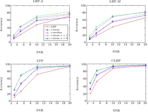
In this paper, some types of average lters are used for noise reduction. Figure 1 illustrates the performance when using four types of average lter for Outex (TC10) dataset. In this gure, the classication accuracy of noisy textures for SNR = 3, 5, 10, and 20 is shown. Also, the results of some lters are shown. Square mean lter (s-mean) uses a square 3 3 mask

for ltering. S-median uses a similar mask, but it calculates the median of 9 points. C-mean is a mean lter that calculates the mean of points on a circular neighborhood (R = 1). It calculates the mean of 9 points that include 8 points on the circle and the center point. It uses the weights = 1 and 8 for the center point. The results are determined for LBP S, LBP M, LTP, and CLBP. The best accuracy is obtained for CLBP. Therefore, in his paper, the results of repeating of the average lter for CLBP are used and they are named Repeat Filter CLBP or RF CLBP.

The plots in Figure 1 indicate that some lters, such as c-mean ( = 1) and s-mean, perform better than c-mean ( = 8) and S-median. The performance of c-mean ( = 1) is similar to that of s-mean. However, for some cases, the performance of c-mean ( = 1) is slightly better than that of s-mean. C-mean requires interpolation step to calculate some points on the circle. Thus, in this paper, s-mean lter is used. 3.1. Repeating average lter

In some methods such as CRLBP [54] mean lter of 3 3 is applied one time to all points of noisy texture to decrease the noise. In this paper, it is shown that if average lter is applied more than one time to a noisy texture, better accuracy of classication can be obtained. In other words, the more value of noise the more number of average lters should be applied to noisy texture. Some feature extraction methods such as LBP use uniform patterns to extract discriminative features of textures. The proposed algorithm is shown

Figure 1. Comparison of the performances of some average lters for noisy Outex (TC10) textures with four variants of LBP (R = 1 and P = 8) and dierent SNR values.

(5)

Figure 2. Pseudo code of estimation of optimum number for repeating the average lter.

in Figure 2. When a texture is corrupted by noise, the percentage of uniform patterns decreases signicantly. However, by using average lter, it is possible to increase this percentage. If average lter is applied to a noisy texture, the percentage of uniform patterns increases. Therefore, by repeating this ltering opera-tion, it is possible to extract more ecient features by LBP operator.

The implementation shows that for low SNR or very noisy textures, the number of repeats of average lter must be high, such as 5 or 6, and for low noise or high SNR, it must be used only one or two. If the number of repeats of using average lter is small, it may not reduce the noise eciently. On the other hand, if this number is too large, it corrupts the texture edges and leads to worse results. Therefore, it is necessary to nd the best number of repetitions. Moreover, it is necessary to use small mask for average lter to save the local edge and contrast of textures. Therefore, in this paper, a 3 3 average mask is used.

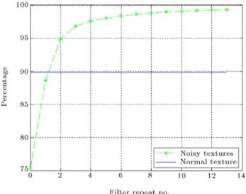
Figures 3 and 4 determine the percentage of uniform patterns of LBP versus the number of repeats of the average mask for Outex and CUReT datasets, respectively. In both of these gures, R = 1 and P = 8. In Figure 3, the percentage of uniform patterns is around 90% without noise. In this gure, SNR = 5. It shows that the percentage of uniform patterns of noisy textures is around 75% and this percentage reaches 88% after the rst time of applying average lter. After the second use of average lter, it reaches 95% and after that, it increases slightly. In addition, Figure 4 shows the similar trend for texture of CUReT. Figures 3 and 4 indicate the uniform percentage

Figure 3. Uniform percentage of LBP S versus number of repeats of average lter for noisy Outex textures (SNR=5).

Figure 4. Uniform percentage of LBP S versus number of repeats of average lter for noisy CUReT textures

(SNR=3).

for a value of SNR. Figure 5 determines the uniform percentage for Outex dataset for dierent values of SNR. In this gure, the uniform percentage for noisy, normal, and ltered textures is shown. The ltered textures are ltered by using average lter for 3, 7, and 10 times. According to this gure, the more number of repeats of average lters, the more percentage of uniform patterns can be obtained.

3.2. Optimum number of repeats for average lter

One of the important points is the optimal number of repeats for the average mask. In addition, average mask decreases the noise in a noisy texture and in-creases the uniform patterns of texture; also, it corrupts some edge and local texture information. Therefore, it is necessary to obtain the optimum or best number for repeating of the average mask. According to Figures 3

(6)

Figure 5. Uniform percentage of Outex for dierent values of SNR.

and 4, the percentage of uniform patterns increases signicantly at the rst, second, and third times of using average mask, but after that it reaches a plateau. Table 1 indicates the summary of implementation for repeating of average mask. It shows the optimum numbers of repeats of average mask for Outex (TC10 and TC13), CUReT, and UIUC datasets. In other words, in this table, the number of repeats to reach the highest accuracy (Max. Acc.) is shown for each SNR value and dataset. In addition, the number of repeats to record the lowest variance of image is determined in Min. Var. columns. It is important to note that the numbers in Table 1 may change for a dierent run of implementation. It is because of random behavior of noise. However, the changes are not large and they may be 1 or 2.

Noise increases the variance of image. On the other hand, using average lter reduces variance. Re-peating average lter decreases the variance of image. In this paper, it is shown that for texture images by repeating average lter the variance decreases, then it increases. Therefore, the average ltering operation should continue until the average variance of each image reaches the minimum value. In other words, the optimum value for repeating average lter is obtained

Figure 6. Variance of ltered noisy image of CUReT dataset versus number of the applications of the lter for SNR = 5.

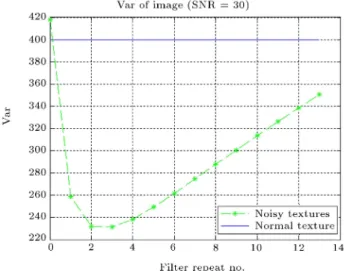
Figure 7. Variance of ltered noisy image of CUReT dataset versus number of the applications of the lter for SNR = 30.

when variance reaches the lowest values. Figures 6 to 9 show the variance (mean variance of all textures) of ltered textures after applying the average lter for 0 to 13 times. These gures indicate that variance of noisy textures decreases, then increases by using

Table 1. The relation between max accuracy and min variance of noisy textures and number of repeats of average lter for dierent SNR values for Outex, CUReT, and UIUC datasets.

SNR

Outex (TC10) Outex (TC13) CUReT UIUC

Max Acc

Min Var

Max Acc

Min Var

Max Acc.

Min Var

Max Acc

Min Var

2 20 5 6 6 14 6 21 90

3 6 5 5 5 7 5 15 105

5 4 3 3 3 5 4 5 115

10 3 2 4 3 2 3 4 110

(7)

Figure 8. Variance of ltered noisy image of Outex (TC10) dataset versus number of the applications of the lter for SNR = 5.

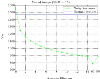
Figure 9. Variance of ltered noisy image of UIUC dataset versus number of the applications of the lter for SNR = 15.

average mask. Figure 6 shows the variance of all noisy textures of CUReT (SNR = 5) versus the number of repeats of average lter. It also determines the variance of normal textures (no noise). According to this gure, the minimum value of variance is obtained when the number of repeats of the lter is four (or may be three or ve). In other words, the best accuracy is obtained when the average lter is applied 4 times to noisy textures. Another example is shown in Figure 7. This gure is same as the previous gure, but SNR is 30. Therefore, the number of repeats should be lower than that in the previous example. Figure 7 indicates that the repeat number 2 or 3 is the best because it provides minimum variance. Also, Figure 8 indicates the same trend for Outex dataset. For some datasets such as Outex and CUReT, the variance decreases

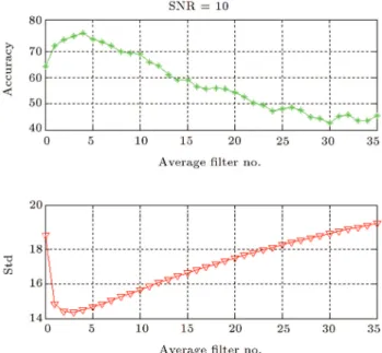
by repeating average lter and after a small number of repeats, it increases. However, for some datasets such as UIUC, it decreases at rst and increases after applying the average lter for more than 200 times. It is indicated in Figure 8. One of the dierences of UIUC and other datasets relates to high variance of UIUC textures. The mean variance of UIUC dataset without noise is around 1480, while it is around 400 for Outex and CUReT. In other words, for some textures such as UIUC that have high variance (without noise), the highest accuracy is not reachable when variance is minimum. For these types of textures, the optimum number for repeating the average lter is obtained when the change of variance is lower than a threshold. Table 1 determines that if the minimum variance is obtained after applying the average lter for k times, the highest accuracy is achieved when the number of repeats is around k. Only for UIUC dataset, this relation is not true. As it is shown in Figure 9, after a large number of repeats, variance increases. However, the maximum accuracy is obtained for lower numbers of repeats. Figures 10 to 12 determine the relation between change of variance and accuracy of RF CLBP (repeating lter CLBP) for Outex (TC10 and TC13) and CUReT datasets for some SNR values. These gures indicate that the accuracy of classication reaches a peak when variance reaches the lowest value. In Figure 10, the max accuracy for TC10 is obtained when n = 6 and variance reaches the lowest value when n = 5. In Figures 10 and 11, the highest accuracy is achieved when n is 4 and 5. In these gures, the minimum value of variance is achieved when n is 4 and 7, respectively. In these gures, the min value of variance is recorded when n is 3 and 5, respectively. However, as it is shown in Figure 13, the

Figure 10. Standard deviation of image and accuracy of RF CLBP of the ltered noisy image of Outex (TC10) dataset versus number of the applications of the lter for SNR = 3.

(8)

Figure 11. Standard deviation of image and accuracy of RF CLBP of the ltered noisy image of Outex (TC13) dataset versus number of the applications of the lter for SNR = 10.

Figure 12. Standard deviation of image and accuracy of RF CLBP of the ltered noisy image of CUReT dataset versus number of the applications of the lter for SNR=3.

trend of change of variance and accuracy for UIUC textures does not follow this relation; UIUC is a dataset that includes high-variance images. For this type of datasets, the optimum number of repeats for the average mask is determined when the change of variance is negligible.

The pseudo code in Figure 2 estimates the optimal number of repeats of the average lter for noisy textures to reach the best accuracy. As it is mentioned in this code, for some textures such as Outex and CUReT of which the average variances are lower than T1 (T1

is around 1000), the average lter should be repeated

Figure 13. Standard deviation of image and accuracy of RF CLBP of the ltered noisy image of UIUC dataset versus number of the applications of the lter for SNR=10.

until the variance of image reaches the lowest value. As illustrated in Figures 6, 7, and 8, the average variance of these textures (without noise) is around 400 (< T1).

For some textures such as UIUC, this value is around 1480 (> T1). It is shown in Figure 9. Therefore,

the optimum number of repeats for average ltering is determined when the change of variance is lower than T 2. The value of this threshold depends on V0; V0 is average variance of all normal textures (without noise). 3.3. Fast average ltering method

In this section, a simple technique is introduced to increase the average ltering. The circular mean lter requires interpolating neighbor points on the circular patch. For the 3 3 area, 4 point values should be interpolated from neighbor points. Therefore, to increase the speed of ltering, square mean lter is used instead of circular mean lter [59] to remove the time of interpolation. It does not have negative eects on the performance, because, as it is shown in Figure 1, the performance of circular mean lter is only slightly better than that of square mean lter.

Here, a simple technique is proposed that in-creases the speed of applying of square lter to an image. If image size is M N, a 3 3 mask should be convolved (M 1)(N 1) times with the image, which takes too much time. To decrease this time, the noisy image I0 should be shifted one pixel to eight directions, by which eight shifted images of I1 to I8 are provided. Then, as in Eq. (6), by calculating the average of all of the 9 images, the ltered image is provided. Iavg

is same as the noisy image that is ltered by 3 3 square mean lter. This method increases the speed of average ltering. The increase in speed depends on the size of each texture. For datasets that are used in

(9)

this paper, using this technique increases the speed of average ltering around 30 times:

Iavg= 1₉ 8

X

i=0

Ii: (6)

4. Experimental results

To determine the performance when repeating average lter, some comprehensive texture datasets are used in this section: the Outex [39], the UIUC [60], and the CUReT [61]. For all noisy textures, Gaussian noise is used.

4.1. Dissimilarity metric method

For comparing two textures, the LBP histograms of them must be compared. There are many methods for comparing two histograms, such as histogram intersec-tion, log-likelihood ratio, and chi-square method [8]. In this paper, chi-square method is used for classication. Eq. (8) shows chi-square method. A test sample, T , is assigned to the class of model, L, that minimizes the chi-square value:

D(T; L) =

N

X

i=1

(Ti Li)2

Ti+ Li ; (7)

where N is the number of bins of each histogram, and Ti and Li are the values of the sample and the

model image at the ith bin, respectively. The nearest neighborhood (K-NN with K = 1) classier with the chi-square distance is used to measure the dissimilarity between two textures.

4.2. Experimental results of the Outex dataset The Outex dataset includes many test suites [39]. These suites have been collected under dier-ent illumination, rotation, and scaling conditions. Outex TC 00010 (TC10) and two groups of Ou-tex TC 00012(TC12(`t') and TC12(`h')) are considered as some famous test suites in this dataset. They can be used for rotation-invariant tests. These two suites have the same 24 classes of textures, which are collected under three dierent illuminates (horizon, inca, and t184) and nine dierent rotation angles (00, 50, 100, 150, 300, 450, 600, 750, and 900).

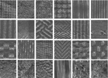
There are 20 non-overlapping 128128 texture im-ages for each class under each condition. Furthermore, in this paper, Outex TC 00013 is used. This suite includes 68 texture classes with the size of 128 128 and inca illumination. Figure 14 shows the 24 images of each class of Outex dataset. Table 2 compares the results of the proposed method and some state-of-the-art noise-robust LBPs. This table and all other tables of this paper compare the results for noisy textures with SNR = 100, 30, 15, 10, 5, 3, and 2.

Figure 14. All 24 classes of Outex dataset.

Table 2 indicates that the RF CLBP with optimal n (number of repeats of the average lter), R = 3, and P = 24 provides the best performance for all values of SNR for TC10. Only for SNR = 3, the accuracy of BRINT1 CS CM is slightly better than that of RF CLBP. The table shows that RF CLBP with n = 1 is same as CRLBP. Therefore, for low noise values, the performance of RF CLBP is same as that of CRLBP, but it is noticeably better than that of BRINT. On the other hand, for low SNR values, the accuracy of RF CLBP with optimum value of n is signicantly higher than that of CRLBP, but the accuracy of BRINT is close to that of RF CLBP. In other words, accuracy of the proposed method is higher than those of both CRLBP and BRINT and other types of noise-robust LBPs for low- and high-noise textures. Tables 3 and 4 show the results of TC12(`t') and TC12(`h'). They also indicate that RF CLBP outperforms all the other methods such as LTP, NTLBP, CRLBP, and BRINT. For very highly noisy textures, only BRINT method provides the accuracy near RF CLBP. For low-noise textures, the accuracy of the proposed method is same as that of CRLBP. In both tables, the best accuracy for all SNR values is obtained by using RF CLBP with optimum number of repeats of lter for R = 3 and P = 24. Only for SNR = 3 and 2, in Table 3, the accuracy of BRINT1 is slightly better than that of RF CLBP.

Figures 15 and 16 show the accuracy of RF CLBP for 2 suites of Outex dataset. In these gures, R = 1 and P = 8. Figure 15(a) shows that the best accuracies of RF CLBP for TC10 when SNR = 30, 10, 5, 3, and 2 are around 3, 3, 4, 5, and 19, respectively. Figure 15(b) determines the performance of RF CLBP for TC12(`t') suites. According to this gure, the highest accuracies for SNR = 30, 10, 5, 3, and 2 are obtained when n (number of repeats of lter) is equal to 2, 2, 3, 4, and 25, respectively. Figure 16(a) determines the same trend for TC13 when R = 1 and P = 8. In this suite,

(10)

Table 2. Classication rates for noisy Outex (TC10) textures using dierent SNR values.

TC10 SNR = 100 SNR = 30 SNR = 15 SNR = 10 SNR = 5 SNR = 3 SNR = 2

LBP 81.09 74.66 64.66 48.78 22.40 10.63 5.55

CLBP S/M/C (R = 1; P = 8) 97.55 96.07 93.65 88.39 51.98 17.79 8.28

CRLBP (R = 1; P = 8) = 1 98.10 97.40 96.43 94.92 83.67 46.09 17.26

CRLBP (R = 1; P = 8) = 8 97.92 97.37 95.91 93.46 74.11 32.03 13.25

CRLBP (R = 3; P = 24) = 1 99.43 99.35 98.93 97.76 92.27 71.96 29.12

CRLBP (R = 3; P = 24) = 8 99.27 98.96 98.26 96.12 85.81 64.23 20.18

NTLBP (MS9) 98.65 96.12 88.85 80.23 51.09 30.34 12.78

LTP 95.91 95.05 88.91 69.01 25.89 12.08 9.32

NRLBP (MS9) 87.40 85.73 80.16 72.42 51.02 32.63 14.01

LBP (MS3) 95.03 86.93 67.24 49.79 24.06 12.97 8.77

BRINT1 CS CM (MS9) 94.74 94.04 92.21 92.42 89.24 77.50 41.38

BRINT2 CS CM (MS9) 97.76 96.48 95.47 92.97 88.31 71.51 38.52

RF CLBP (R = 1; P = 8; n = 1) 97.14 96.80 95.63 93.46 79.87 44.27 15.00 RF CLBP (R = 1; P = 8; n = 2) 98.20 97.55 96.64 96.61 87.81 59.43 23.57 RF CLBP (R = 1; P = 8; n = opt) 98.49 98.33 97.97 96.82 91.90 76.49 40.12 RF CLBP (R = 3; P = 24; n = 1) 99.43 99.40 98.98 98.54 92.71 70.95 28.59 RF CLBP (R = 3; P = 24; n = 2) 99.19 99.22 98.96 98.75 94.58 76.16 31.30 RF CLBP (R = 3; P = 24; n = opt) 99.43 99.40 98.98 98.78 94.58 77.48 43.35

Table 3. Classication rates for noisy Outex (TC12(`t')) textures using dierent SNR values.

TC12t SNR = 100 SNR = 30 SNR = 15 SNR = 10 SNR = 5 SNR = 3 SNR = 2

LBP 71.27 64.56 53.38 42.18 20.86 9.88 5.63

CLBP S/M/C (R = 1; P = 8) 90.93 87.41 84.05 79.77 48.73 18.19 8.19

CRLBP (R = 1; P = 8) = 1 93.84 91.71 90.56 87.29 75.39 42.89 13.98

CRLBP (R = 1; P = 8) = 8 92.57 91.06 89.44 83.47 65.16 27.41 28.02

CRLBP (R = 3; P = 24; N = 46) = 1 97.34 97.08 96.50 94.91 87.97 66.34 27.01 CRLBP (R = 3; P = 24; N = 46) = 8 96.46 96.41 95.28 92.69 79.61 52.92 21.54

NTLBP (MS9) 92.15 89.35 83.77 74.47 49.84 31.27 12.01

LTP 80.76 80.30 75.42 60.14 24.93 11.09 6.5

NRLBP (MS9) 84.49 81.16 77.52 70.16 50.88 33.31 13.87

LBP (MS3) 91.30 82.55 60.25 47.31 24.07 13.63 8.55

BRINT1 CS CM (MS9) 92.87 90.63 89.72 88.12 83.84 74.47 38.55

BRINT2 CS CM (MS9) 95.95 93.59 91.32 90.49 83.68 69.70 35.01

(11)

Table 4. Classication rates for noisy Outex (TC12(`h')) textures using dierent SNR values.

TC12h SNR = 100 SNR = 30 SNR = 15 SNR = 10 SNR = 5 SNR = 3 SNR = 2

LBP 68.06 64.03 55.58 45.02 21.37 10.37 6.09

CLBP S/M/C (R = 1; P = 8) 92.52 90.53 86.90 81.78 50.60 17.87 7.31

CRLBP (R = 1; P = 8) = 1 94.12 92.66 90.44 88.40 77.45 43.17 12.08

CRLBP (R = 1; P = 8) = 8 93.91 93.50 90.35 85.93 70.56 29.56 22.50

CRLBP (R = 3; P = 24; N = 46) = 1 96.44 97.04 96.57 95.49 88,06 63.22 23.88 CRLBP (R = 3; P = 24; N = 46) = 8 95.63 95.88 94.98 93.59 79.68 42.88 19.87

NTLBP (MS9) 94.35 90.81 84.95 75.49 47.04 30.38 12.04

LTP 80.84 79.23 75.28 64.68 25.42 10.74 7.23

NRLBP (MS9) 85.76 82.69 77.38 69.68 49.07 32.06 11.44

LBP (MS3) 90.72 79.17 60.74 45.81 25.02 12.55 9.87

BRINT1 CS CM (MS9) 94.10 92.31 90.95 89.84 85.83 76.04 34.15

BRINT2 CS CM (MS9) 96.92 95.14 93.66 92.29 84.77 71.02 32.56

Figure 15. The performance of RF CLBP (R = 1, P = 8) for dierent numbers of repeats of average lter for noisy Outex Dataset: (a) TC10 and (b) TC12(t).

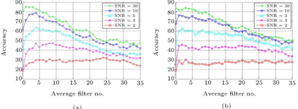
Figure 16. The performance of RF CLBP for dierent numbers of repeats of average lter for noisy Outex (TC13): (a) R = 1, P = 8 and (b) R = 3, P = 24.

(12)

when SNR = 30, the highest accuracy is obtained for n = 1, but it is 4 for SNR = 10. Furthermore, the best performances for SNR = 5, 3, and 2 are achieved when n = 4, 4, and, 19 respectively. All of the plots in Figures 15 and 16(a) use RF CLBP with R = 1 and P = 8. The performance of RF CLBP improves for larger neighborhoods with the similar trend. The performance of RF CLBP for R = 3 and P = 24 is shown in Figure 16(b). This plot indicates that the best numbers of repeats for SNR = 30, 10, 5, 3, and 2 are achieved when n is 3, 1, 2, 2, and 3, respectively. Figures 15 and 16 show that for large values of SNR, the best performance is achieved after 1, 2, or at max, 3 times of using average lter while for high noisy textures, it is necessary to repeat the lter more times. Furthermore, after some special number of using average lter, the accuracy decreases. However, this reduction is moderate for large neighborhood.

Some methods such as GLCM that use co-occurrence matrix are not rotation-invariant and they are sensitive to noise. Therefore, if they are used for these textures, the classication accuracy decreases signicantly [55].

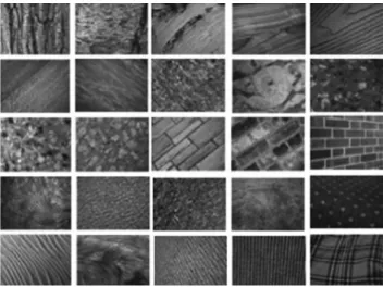
4.3. Experimental results of the UIUC dataset The UIUC dataset [60] contains 25 classes with 40 images in each class. Resolution of each texture image is 640480. Figure 17 shows one image for each class of UIUC dataset. For implementation, each time, N = 20 images of each class are selected randomly for train and the rest of them (40 N) are used for test. This operation is run 100 times and the average of the results is shown in Table 5. This table compares the accuracy of the proposed method with those of LBP, LTP, CLBP, and CRLBP. In this table, for all values of SNR, the highest performance is achieved by using RF CLBP when R = 3 and P = 24 for optimum value of n. Also,

Figure 17. All 25 classes of UIUC dataset.

RF CLBP with R = 1 and P = 8 has the second best performance in this table.

As it is mentioned before, CRLBP is same as RF CLBP with n = 1. Therefore, these two methods are almost the same considering accuracy for low-noise textures; however, for highly noisy textures, the accuracy of RF CLBP is higher by far than those of all CRLBP and all other LBP variants such as LTP, LBP, and CLBP. Also, the results of LBP-based and non-LBP methods when used for UIUC textures are shown in Table 6 in the next sections.

4.4. Experimental results of the CUReT dataset

The CUReT dataset [61] contains 61 classes of tex-tures. They are shown in Figure 18. These images are captured in dierent viewpoints and illumination orientations. For each class, 92 images are selected from the images that have a viewing angle of less than 60_{. Each time, N = 46 images are randomly}

Table 5. Classication rates for noisy UIUC textures using dierent SNR values. (N = 20).

UIUC SNR = 100 SNR = 30 SNR = 15 SNR = 10 SNR = 5 SNR = 3 SNR = 2

LBP (R = 1) 54.40 57.30 54.35 48.16 44.08 41.15 42.18

LTP (R = 1) 76.88 77.44 73.00 66.14 62.47 60.24 59.12

CLBP S/M/C (R = 1; P = 8; N = 20) 87.42 87.68 84.68 81.44 72.48 71.76 66.47 CLBP S/M/C (R = 3; P = 24; N = 20) 90.74 90.38 87.56 81.64 74.54 73.85 68.23 CRLBP (R = 3; P = 24; N = 20) = 1 93.49 93.08 92.74 88.57 80.20 76.55 70.55 CRLBP (R = 3; P = 24; N = 20) = 8 92.51 92.28 91.11 85.90 77.16 73.12 68.85 RF CLBP (R = 1; P = 8; n = 1) 89.55 89.38 88.20 87.91 81.78 75.12 68.51 RF CLBP (R = 1; P = 8; n = 2) 89.84 89.77 90.00 89.41 85.31 78.03 70.24 RF CLBP (R = 1; P = 8; n = opt) 90.21 90.03 90.17 90.19 87.13 82.72 75.70 RF CLBP (R = 3; P = 24; n = 1) 93.73 93.15 92.82 89.81 81.27 76.93 70.40 RF CLBP (R = 3; P = 24; n = 2) 94.52 94.44 94.64 94.10 89.87 81.85 75.01 RF CLBP (R = 3; P = 24; n = opt) 94.82 94.80 94.64 94.28 92.32 87.19 82.77

(13)

Table 6. Classication rates for 3 datasets of textures.

Methods Outex UIUC (N = 20) CUReT (N = 46)

LBP 81.19 54.51 77.54

CLBP S/M/C (R = 1; P = 8) 97.66 87.52 95.56

CRLBP (R = 1; P = 8) = 1 98.12 93.54 94.70

CRLBP (R = 1; P = 8) = 8 97.97 92.58 95.58

CRLBP (R = 3; P = 24) = 1 99.42 93.65 96.21

CRLBP (R = 3; P = 24) = 8 99.34 92.57 96.42

NTLBP (MS9) 98.77 | 91.64

LTP 95.98 76.94 84.92

BRINT1 CS CM (MS9) 94.80 | 96.85

BRINT2 CS CM (MS9) 97.87 | 96.80

RF CLBP (R = 1; P = 8; n = 1) 97.24 89.57 96.07 RF CLBP (R = 1; P = 8; n = 2) 98.21 89.88 95.28 RF CLBP (R = 1; P = 8; n = opt) 98.54 90.26 96.06 RF CLBP (R = 3; P = 24; n = 1) 99.44 93.75 95.99 RF CLBP (R = 3; P = 24; n = 2) 99.21 94.62 95.15 RF CLBP (R = 3; P = 24; n = opt) 99.45 94.83 96.11

GLCM 83.02 75.67 |

GLCM, pyramid decomposition 84.61 73.99 |

GLCM, Gaussian smoothing 81.79 81.88 |

Multi scale GLCM 89.40 81.76 |

Gabor 84.90 69.90 87.50

VZ Joint 98.51 80.20 96.59

VZ MR8 94.06 92.14 95.75

Lazebnik (H + L)(S + R) | 95.42 72.50

HA+SIFT | 97.50 89.10

Figure 18. All 61 classes of CUReT dataset.

chosen for train from each class. The remaining (92 N) images are used as test samples. The average classication rates over 100 random tests are shown in Table 7.

In Table 7, the comparison between the proposed methods and some LBP noise-resistant methods such as BRINT, CRLBP, LTP, DLBP, and NTLBP is illus-trated. The wavelet transform features (DBWP) [23] and Circular Gaussian MRFs (ACGMRF) [12] are other two methods that are illustrated in the table. The results of some Gabor lter methods such as

TGF [17], CGF [18], and NGF [19] are shown in this table. Furthermore, DLBP+NGF is a method that uses Dominant LBP (DLBP) [19] with normal Gabor lter. It can be seen in the table that for all SNR < 100 values, the proposed method provides the best accuracy. Only for SNR = 100, the performance of BRINT1 CS CM (MS9) is slightly higher than that of RF CLBP. Similar to Outex dataset, in CUReT dataset, the accuracy of RF CLBP is slightly better than that of CRLBP for low noise. Also, this accuracy is slightly better than that of BRINT for highly noisy textures. However, for high SNR values, accuracy of the proposed method is signicantly higher than that of BRINT. On the other hand, this performance is noticeably more accurate than that of CRLBP for very noisy textures.

As it is mentioned in some papers [55], the performance of Gabor lter and co-occurrence matrix methods signicantly declines for noisy textures. Ta-ble 7 shows some of these results.

4.5. Comparison for normal textures (without noise)

In this section, the comparison between accuracy of the proposed method and accuracy of some LBP-based, co-occurrence, Gabor Filter, patch LBP-based, and general descriptor approaches is shown. Table 6 shows

(14)

Table 7. Classication rates for noisy CUReT textures using dierent SNR values (N = 46).

CUReT SNR = 100 SNR = 30 SNR = 15 SNR = 10 SNR = 5 SNR = 3 SNR = 2

LBP 77.47 73.25 67.50 62.72 50.25 39.72 25.78

CLBP S/M/C (R = 1; P = 8; N = 46) 95.49 94.42 91.97 88.11 77.91 66.30 50.34 CLBP S/M/C (R = 3; P = 24; N = 46) 95.51 95.87 87.23 72.77 61.35 57.77 54.20 CRLBP (R = 3; P = 24; N = 46) = 1 96.06 95.90 93.56 85.58 79.67 74.55 61.22 CRLBP (R = 3; P = 24; N = 46) = 8 96.34 96.18 92.30 82.88 74.97 69.98 57.55

NTLBP (MS9) 91.56 85.99 78.98 74.90 65.74 56.31 39.45

LTP 84.82 84.06 79.60 72.89 57.62 47.13 37.27

LTP (MS9) 92.22 90.15 86.66 84.55 77.48 70.67 41.05

BRINT1 CS CM (MS9) 96.81 95.39 93.69 90.92 86.11 80.45 64.87

BRINT2 CS CM (MS9) 96.78 94.90 92.83 90.46 84.48 78.33 63.21

DBWP 88.37 85.33 80.38 71.40 63.40 | |

TGF 60.79 62.69 51.80 43.67 46.41 | |

CGF 52.94 53.39 52.36 46.39 46.74 | |

ACGMRF 66.90 57.54 51.36 47.05 47.08 | |

NGF 47.86 45.49 43.14 41.63 40.06 | |

DLBP 87.82 85.28 79.44 68.73 47.72 | |

DLBP+NGF 96.17 95.78 92.81 86.06 71.28 | |

the results of the proposed method and some other methods for 3 datasets. In this table, the methods which are related to 4 groups of texture classication are shown: GLCM method, a Gabor method, two scale-invariant and patch-based methods of VZ Joint and VZ MR8 [62,63], and general descriptor methods that include Lazebnik [64] and SIFT [34]. This table shows the results of texture classication without noise. If noise is added to the texture, the accuracy of classication of some methods considerably decreases. According to this table, the best accuracy for Outext is obtained by the proposed method. HA+SIFT provides the best accuracy for UIUC. However, the SIFT-based methods are very time consuming approaches. For CUReT textures, BRINT1 CS CM (MS9) achieves the best classication accuracy. This method uses multi resolution parameters for an especial version of LBP. MS9 refers to the 9 dierent combinations of R and P (LBP parameters). This table shows that the accuracy of the proposed method is noticeably higher than that of Gabor and co-occurrence based methods (GLCM).

General descriptors such as SIFT and Lazeb-nik [64] achieve high accuracy only for UIUC textures. These types of textures have large numbers of key

points; therefore, their accuracy is high. The accuracy of general descriptors such as SIFT decreases for some textures such as CUReT. This dataset contains some textures that have low contrast. Therefore, number of key points of some CUReT textures is very low. For the default threshold of SIFT, the number of key points of some CUReT textures is zero.

4.6. Comparison with other average ltering methods

In this paper, it is shown that repeating the mean lter decreases the noise and increases the classication accuracy of textures. A 3 3 square mean lter is used in the proposed method. The size of window must be small for better description of edge details and avoidance of corruption of edge and details of textures. The smallest size of window that is symmetric is 3 3. Thus, it was selected for this paper. If a larger size had been selected, it would have corrupted the edge and local details of textures. There are some other average ltering methods that remove noise from im-age. Nagao [65] and improved Nagao [66] are two types of these methods. These methods preserve edge and textures details better than simple mean method. If

(15)

they had been used instead of the proposed method, the classication accuracy would have slightly increased, but the computational time would have been very high. In this section, the computational times of the proposed method and these two methods are compared.

Table 8 determines that the proposed fast mean method increases the speed of mean square method around 30 times. Table 9 shows the time of feature ex-traction for some methods [24]. This table determines the time of feature extraction for 2 datasets. According to this table, the proposed method (RF CLBP with the proposed fast mean) is considerably faster than other methods.

Some average spatial lters have been proposed for noise reduction. Nagao [65] is one of these methods. The idea of Nagao lter is as follows: rstly, a rectangle template around the central pixel is rotated and the position of minimum variance as the default direction template is chosen; then, the value of the central pixel is replaced by the average value of the default template. Such processes are iterated until the pixels do not vary. The performance of Nagao lter depends on the shape of its template. The computational time of Nagao lter is also very high. The eect of Nagao lter is not satisfying for its mean lter style [66]. Therefore, Zhang and Wu proposed the improved Nagao lter or window-length Nagao lter (AWN) method [66]. They

Table 8. Average time of mean and the proposed fast mean for a texture (msec).

Mean Proposed

fast mean Ratio

UIUC 2562.5 72.6 35.29

Outex (TC10) 78.71 2.57 30.62

CUReT 52.33 1.84 28.44

showed that by using median lter instead of mean lter and some techniques, the edge and some other details of image were preserved and better performance than that of Nagao method could be obtained.

Both Nagao and AWN methods can preserve edge and textures details better than simple mean method. But, the computational times of theme are considerably higher than that of mean method. As it is shown in Table 8, the proposed fast mean method increases the speed of square mean method around 30 times in comparison with the traditional mean lter. Nagao lter is slower than simple mean lter at least 10 times. In other words, speed of the proposed fast mean method is higher than that of Nagao around 300 times. For improved Nagao (AWN) method, median or complex templates are used; therefore, the speed of AWN is lower than that of Nagao and the ratio is higher than 300 for AWN method.

4.7. Comparison with other methods considering LBP specications

Table 10 compares specications of some texture fea-tures extraction methods. In this paper, the LBP with riu2 mapping is used. It is shown in the table that local binary pattern (riu2) is a rotation-invariant and gray-scale-invariant method [67]. The computational time of this method is low and it extracts a small number of features. However, LBP is not scale-invariant and sensitive to noise. The proposed method and some advanced LBPs [55] provide noise robustness for LBP. It is a simple method that can be combined with other methods and it has achieved high performance in classication results for many kinds of texture datasets [39]. It has been extensively exploited in many applications, e.g. face image analysis, image and video retrieval, environment modeling, visual inspection,

mo-Table 9. Computational time (sec) required for feature extraction. Dataset LBP CLBP RF CLBP

(n = 1)

RF CLBP fast mean (n = 1)

Gabor GLCM

Multi scale GLCM UIUC 24.95 37.20 284.50 44.70 1371.59 39.35 183.10

Outex 1.89 4.93 21.56 5.45 297.94 41.66 180.49

Table 10. Comparison between LBP and other approaches.

Simple LBP LBPriu2 _CLBPriu2 _Proposed _SIFT _GLCM _Gabor

Gray-scale-invariant Yes Yes Yes Yes Yes No Yes

Rotate-invariant No Yes Yes Yes Yes No Yes

Scale-invariant No No No No Yes No Yes

Noise robustness No No No Yes Yes No No

Computational time Medium Low Low Low Very high Medium High

(16)

tion analysis, biomedical and aerial image analysis, and remote sensing [68]. Some methods such as [69] extract features which are robust not only to the noise but also to the change of noise.

5. Conclusion

In this paper, it is shown that repeating average lter for noisy texture increases the classication accuracy signicantly. The more value of noise, the more number of repeats of average lter should be used for noisy textures. The optimal value for repeating the average lter is obtained when variance of texture reaches the lowest values or the change of it is smaller than a threshold value. The performance of the proposed method is better than that of some novel and advanced noise-robust LBP methods. Some state-of-the-art methods such as CRLBP provide good performance only for highly SNR noisy textures. On the other hand, some advanced methods such as BRINT provide high accuracy for low SNR values. The proposed method provides the best performance for both low and high SNR values. Furthermore, by using the fast technique that is proposed in this paper, the speed of applying average lter increases signicantly. Therefore, the speed of the proposed method is by far higher than those of almost all the noise-robust LBP methods that are used in this paper. The proposed method is used as a preprocessing operation for noisy textures. After this pre-processing operation, CLBP is used for feature extraction. It is possible to use any other types of feature extraction methods to extract features of textures.

References

1. Cohen, F.S., Fan, Z. and Attali, S. \Automated inspection of textile fabrics using Textural models", IEEE Transactions on Pattern Analysis and Machine Intelligence, 13(8), pp. 803-808 (1991).

2. Tajeripour, F., Kabir, E. and Sheikhi, A. \Fabric defect detection using modied local binary patterns", EURASIP Journal on Advances in Signal Processing, 8, pp. 1-12 (2008).

3. Ji, Q., Engel, J. and Craine, E. \Texture analysis for classication of cervix lesions", IEEE Transactions on Medical Imaging, 19(11), pp. 1144-1149 (2000).

4. Anys, H. and He, D.C. \Evaluation of textural and multi polarization radar features for crop classica-tion", IEEE Transactions on Geoscience and Remote Sensing, 33(5), pp.1170-1181 (1995).

5. Zhang, B., Gao, Y., Zhao, S. and Liu, J. \Local derivative patterns versus local binary patterns: face recognition with high-order local patterns descriptor", IEEE Transactions on Image Processing, 19(2), pp. 533-544 (2010).

6. Murala, S., Maheshwari, R.P. and Subramanian, R.B. \Local tetra patterns: a new feature descriptor for content-based image retrieval", IEEE Transactions on Image Processing, 21(5), pp. 2874-2886 (2012).

7. Haralik, R.M., Shanmugam, K. and Dinstein, I. \Tex-ture fea\Tex-tures for image classication", IEEE Transac-tions on Systems, Man and Cybernetics, 3(6), pp. 610-621 (1973).

8. Ojala, T., Pietikainen, M. and Maenpa, T.T. \Mul-tiresolution gray-scale and rotation Invariant texture classication with local binary patterns", IEEE Trans-actions on Pattern Analysis and Machine Intelligence, 24(7), pp. 971-987 (2002).

9. Chen, J.L. and Kundu, A. \Rotation and gray scale transform invariant texture identication using wavelet decomposition and hidden Markov model", IEEE Transactions on Pattern Analysis and Machine Intel-ligence, 16(2), pp. 208-214 (1994).

10. Campisi, P., Neri, A., Panci, C. and Scarano, G. \Ro-bust rotation-invariant texture classication using a model based approach", IEEE Transactions on Image Processing, 13(6), pp. 782-791 (2004).

11. Kashyap, R.L. and Khotanzad, A. \A model-based method for rotation invariant texture classication", IEEE Transactions on Pattern Analysis and Machine Intelligence, 8(4), pp. 472-481 (1986).

12. Deng, H. and Clausi, D.A. \Gaussian MRF rotation-invariant features for image classication", IEEE Trans. Pattern Anal. Mach. Intell., 26(7), pp. 951-955 (2004).

13. Chellappa, R. and Chatterjee, S., \Classication of textures using Gaussian Markov random elds", IEEE Trans. Acoust., Speech, Signal Process., ASSP-33, 4, pp. 959-963 (1985).

14. Eichmann, G. and Kasparis, T. \Topologically invari-ant texture descriptors", Computer Vision, Graphics and Image Processing, 41(3), pp. 267-281 (1988).

15. Lam, W.K. and Li, C. \Rotation texture classication by improved iterative morphological decomposition", IEEE Proceedings Vision, Image and Signal Process-ing, 144(3), pp. 171-179 (1997).

16. Daugman, J.G. \Uncertainty relation for resolution in space, spatial frequency, and orientation optimized by two dimensional visual cortical lters", Journal of the Optical Society of America, pp. 1160-1169 (1985).

17. Bovik, A.C., Clark, M. and Geisler, W.S. \Multi-channel texture analysis using localized spatial lters", IEEE Trans. Pattern Anal. Mach. Intell., 12(1), pp. 55-73 (1990).

18. Haley, G.M. and Manjunath, B.S. \Rotation-invariant texture classication using a complete space-frequency model", IEEE Trans. Image Process., 8(2), pp. 255-269 (1999).

19. Liao, S., Law, M.W.K. and Chung, A.C.S. \Dominant local binary patterns for texture classication", IEEE Trans. on Image Processing, 18(5), pp. 1107-1118 (2009).

(17)

20. Arof, H. and Deravi, F. \Circular neighborhood and1-DDFT features for texture classication and segmen-tation", IEEE Proceedings Vision, Image, and Signal Processing, 145(3), pp. 167-172 (1998)

21. Kim, S. \Texture classication using rotation wavelet lters", IEEE Transactions on Systems, Man and Cybernetics, Part A: Systems and Humans, 30(6), pp. 847-852 (2000).

22. Kokare, M., Biswas, P.K. and Chatterji, B.N. \Rotation-invariant texture image retrieval using ro-tation complex wavelet lters", IEEE Transactions on Systems, Man and Cybernetics, Part B: Cybernetics, 36(6), pp. 1273-1282 (2006).

23. Mallat, S.G. \A theory for multiresolution signal decomposition: The wavelet representation", IEEE Trans. Pattern Anal. Mach. Intell., 11(7), pp. 674-693 (1989).

24. Siqueira, F.R., Schwartz, W.R. and Pedrini, H. \Multi-scale gray level co-occurrence matrices for texture description", Neurocomputing, pp. 336-345 (2013).

25. Clausi, D. and Jernigan, M. \A fast method to deter-mine co-occurrence texture features", IEEE Transac-tions on Geoscience and Remote Sensing, 36(1), pp. 298-300 (1998).

26. Gelzinis, A., Verikas, A. and Bacauskiene, M. \In-creasing the discrimination power of the co-occurrence matrix-based features", Pattern Recognition, 40(9), pp. 2367-2372 (2007).

27. Walker, R., Jackway, P. and Longsta, D. \Genetic algorithm optimization of adaptive multi-scale GLCM features", International Journal of Pattern Recogni-tion and Articial Intelligence, 17(1), pp. 17-39 (2003).

28. Benco, M. and Hudec, R. \Novel method for color textures features extraction based on GLCM", Radio Engineering, 4(16), pp. 64-67 (2007).

29. Hu, Y. \Unsupervised texture classication by com-bining multi-scale features and K-means classier", In Chinese Conference on Pattern Recognition, pp. 1-5 (2009).

30. Pacici, F. and Chini, M. \Urban land-use multi-scale textural analysis", In IEEE International Geoscience and Remote Sensing Symposium, pp. 342-345 (2008).

31. Rakwatin, P., Longepe, N., Isoguchi, O., Shimada, M. and Uryu, Y. \Mapping tropical forest using ALOS PALSAR 50 m resolution data with multiscale GLCM analysis", In IEEE International Geoscience and Remote Sensing Symposium, pp. 1234-1237 (2010).

32. Nguyen-Duc, H., Do-Hong, T., Le-Tien, T. and Bui-Thu, C. \A new descriptor for image retrieval using contourlet co-occurrence", In Communications and Electronics (ICCE), Third International Conference, pp. 169-174 (2010).

33. Do, M., Vetterli, M., The Contourlet Transform: 552 \An ecient directional multi resolution image repre-sentation", IEEE Transactions on Image Processing, 14(12), pp. 2091-2106.

34. Lowe, D.G. \Distinctive image features from scale-invariant keypoints", International Journal of Com-puter Vision, 60, pp. 91-110 (2004)

35. Bay, H., Tuytelaars, T. and Van Gool, L. \SURF: speeded-up robust features", In European Conference on Computer Vision, pp. 346-359 (2006).

36. Dalai, N., Triggs, B., Rhone-Alps, I. and Montbonnot, F. \Histograms of oriented gradients for human detec-tion", In IEEE Conference on Computer Vision and Pattern Recognition, pp. 886-893 (2005).

37. Mikolajczyk, K. and Schmid, C. \A performance evaluation of local descriptors", IEEE Transactions on Pattern Analysis and Machine Intelligence, 27(10), pp.1615 -1630 (2005).

38. Ojala, T., Pietikainen, M. and Harwood, D.A. \Com-parative Study of texture measures with classication based on feature distributions", Pattern Recognition, 29(1), pp. 51-59 (1996).

39. Ojala, T., Maenpaa, T., Pietikainen, M., Viertola, J., Kyllonen, J. and Huovinen, S. \Outex - new framework for empirical evaluation of texture analysis algorithm", in Proc. International Conference on Pattern Recogni-tion, pp. 701-706 (2002).

40. Ahonen, T., Hadid, A. and Pietikainen, M. \Face recognition with local binary patterns: application to face recognition", IEEE Trans. on Pattern Anal-ysis and Machine Intelligence, 28(12), pp. 2037-2041 (2006).

41. Zhao, G. and Pietikainen, M. \Dynamic texture recog-nition using local binary patterns with an applica-tion to facial expressions", IEEE Trans. on Pattern Analysis and Machine Intelligence, 27(6), pp. 915-928 (2007).

42. Huang, X., Li, S.Z. and Wang, Y. \Shape localization based on statistical method using extended local bi-nary patterns", In Proc. International Conference on Image and Graphics, pp. 184-187 (2004).

43. Zabih, R. and Wood, J. \Non-parametric local trans-forms for computing visual correspondence", In Proc. Euro. Conf. Comput. Vis., pp. 151-158 (1994).

44. Ojala, T. \Nonparametric texture analysis using sim-ple spatial operators, with applications in visual in-spection", Acta Universitatis Oulue nsis, C 105 (1997).

45. Pietikainen, M., Ojala, T. and Xu, Z. \Rotation-invariant texture classication using feature distribu-tions", Pattern Recognition, 33(1), pp. 43-52 (2000).

46. Jin, H., Liu, Q., Lu, H. and Tong, X. \Face detection using improved LBP under Bayesian framework", In Proceedings of the 3rd International Conference on Image and Graphics, ICIG 2004, pp. 306-309 (2004).

47. Tan, X. and Triggs, B. \Enhanced local texture feature sets for face recognition under dicult lighting condi-tions", In Proc. International Workshop on Analysis and Modeling of Faces and Gestures, pp. 168-182 (2007).

(18)

48. Iakovidis, D.K., Keramidas, E.G. and Maroulis, D. \Fuzzy local binary patterns for ultra sound texture characterization", In Proceedings of the 5th Interna-tional Conference on Image Analysis and Recognition, ICIAR 2008, 5112 of Lecture Notes in Computer Sci-ence, Povoa de Varzim, Portugal, pp. 750-759 (2008).

49. Ahonen, T. and Pietikainen, M. \Soft histograms for local binary patterns", In Proceedings of the Finnish Signal Processing Symposium, FINSIG 2007, 1, Oulu, Finland, pp. 1-4 (2007).

50. Haane, A., Seetharaman, G. and Zavidovique, B. \Median binary pattern for textures classication", In Proceedings of the 4thInternational Conference, ICIAR 2007, 4633 of Lecture Notes in Computer Science, Montreal, Canada, pp. 387-398 (2007).

51. Fathi, A. and Naghsh-Nilchi, A.R. \Noise tolerant local binary pattern operator for ecient texture analysis", Pattern Recognit. Letters, 33(9), pp. 1093-1100 (2012).

52. Ren, J., Jiang, X. and Yuan, J. \Noise resistant local binary pattern with an embedded error correction mechanism", IEEE Trans. Image Process., 22(10), pp. 4049-4060 (2013).

53. Liu, L., Long, Y., Fieguth, P., Lao, S. and Zhao, G. \BRINT: Binary rotation invariant and noise tolerant texture classication", IEEE Trans. on Image Process-ing (2014).

54. Zhao, Y., Jia, W., XiangHuc, R. and Min, H. \Completed robust local binary pattern for texture classication", Neurocomputing, 106, pp. 68-76 (2013).

55. Kylberg G. and Sintorn I.M. \Evaluation of noise ro-bustness for local binary pattern descriptors in texture classication", EURASIP Journal on Image and Video Processing, 17, pp. 1-20 (2013).

56. Zhang, Y., Wang, S., Ji, G. and Phillips, P. \Fruit classication using computer vision and feed forward neural network", Journal of Food Engineering, 143, pp. 167-177 (2014).

57. Unser, M. \Texture classication and segmentation using wavelet frames", IEEE Transaction on Image Processing, 4(11), pp. 1549-1560 (1995).

58. Guo, Z., Zhang, L. and Zhang, D. \A completed modeling of local binary pattern operator for texture classication", IEEE Trans. Image Process., 9(16), pp. 1657-1663 (2010).

59. Shakoor, M.H. and Tajeripour, F. \Circular mean ltering for textures noise reduction", Iranian Journal of Electrical & Electronic Engineering, 11(3), pp. 195-203 (2015).

60. Lazebnik, S., Schmid, C. and Ponce, J. \A sparse tex-ture representation using local ane regions", IEEE Trans. Pattern Anal. Mach. Intell., 27(8), pp. 1265-1278 (2005).

61. Dana, K.J., Ginneken, B., Nayar, S.K. and Koen-derink, J.J. \Reectance and texture of real world

surfaces", ACM Transactions on Graphics, 18(1), pp. 1-34 (1999).

62. Varma, M. and Zisserman, A. \A statistical approach to texture classication from single images", Interna-tional Journal of Computer Vision, 62(1), pp. 61-81 (2005).

63. Varma, M. and Zisserman, A. \A statistical approach to material classication using image patch exem-plars", IEEE Transactions on Pattern Analysis and Machine Intelligence, 31(11), pp. 2032-2047 (2009).

64. Lazebnik, S., Schmid, C. and Ponce, J. \A sparse tex-ture representation using local ane regions", IEEE Trans. Pattern Anal. Mach. Intell., 27(8), pp. 1265-1278 (2005).

65. Makoto, N. and Takashi, M. \Edge preserving smooth-ing", Computer Graph Imag Proc, 9, pp. 394-407 (1979).

66. Zhang, Y. and Wu, L. \Improved image lter based on SPCNN", Science in China Series F-Information Sciences, 51(12), pp. 2115-2125 (2008).

67. Maani, R., Karla, S. and Yang, Y. \Noise robust rotation invariant features for texture classication", Pattern Recognition, 46, pp. 2103-2116 (2013).

68. Huang, D., Shan, C., Ardabilian, M., Wang, Y. and Chen, L. \Local binary patterns and its application to facial image analysis: A survey", IEEE Transactions on Systems Man, and Cybernetics, 4(5), pp. 765-781 (2011).

69. Shakoor, M.H. and Tajeripour, F. \Noise robust and rotation invariant entropy features for texture classi-cation", Multimedia Tools and Applications, 75(6), pp. 1-36 (2016). DOI 10.1007/s11042-016-3455-6

Biographies

Mohammad Hossein Shakoor received the BS de-gree in Computer Engineering from Shiraz University, Shiraz, Iran, in 1998, and MS degree in Computer Architecture from Isfahan university, Isfahan, Iran, in 2003. Currently, he is pursuing PhD in Computer Engineering with the specialty of Articial Intelligence at Shiraz University. His research interests include tex-ture classication, pattern recognition, and computer vision.

Farshad Tajeripour received the BS and MS degrees in Electronic Engineering from Shiraz University, Shi-raz, Iran, in 1994 and 1997, respectively. He received PhD degree in Electronic Engineering from Tarbiat Modarres University, Tehran, Iran, in 2009. Currently, he is an Assistant Professor at Shiraz University. His research interests include texture classication, pattern recognition, computer vision, and video processing.