Vol 6, No 6 (2015)

(1)

Available online throug

ISSN 2229 – 5046

SYNCHRONIZATION OF THREE DIMENSIONAL CANCER MODEL

WITH ROSSLER SYSTEM USING A ROBUST ADAPTIVE SLIDING MODE CONTROLLER

WITH APPLICATION TO SECURE COMMUNICATIONS

MOHAMMAD SHAHZAD

Department of General Requirements, College of Applied Sciences, Nizwa, Oman.

MOHAMMED RAZIUDDIN*

Research Scholar, Singhania University, Jhunjhunu, Rajasthan, India.

(Received On: 10-05-15; Revised & Accepted On: 26-06-15)

ABSTRACT

T

his paper deals the computational study of synchronization of the Three Dimensional Cancer Model (TDCM) with Rossler System (RS) using a Robust Adaptive Sliding Mode Controller (RASMC) together with uncertainties, external disturbances and fully unknown parameters. A simple suitable sliding surface, which includes synchronization errors, is constructed and appropriate update laws are used to tackle the uncertainties, external disturbances and unknown parameters. All simulations to achieve the synchronization for the proposed technique for the two nonidentical chaotic systems under consideration are being done using Mathematica. Furthermore, application of synchronization to secure communication is also demonstrated on tumour cells.

Key Words: TDCM; Synchronization; RASMC.

1. INTRODUCTION

Synchronization of chaotic systems is a collective phenomenon occurring in systems of interacting units, and is ubiquitous in nature, society and technology. Recent studies have enlightened the important role played by the interaction topology on the emergence of synchronized states. It gained momentum in the last two decades and various techniques have been proposed on synchronization of chaotic systems [1–8]. The aforecited works on chaos synchronization have focused on chaotic systems without model uncertainties and external disturbances. It has been observed practically that structural variations of the systems and unmodeled dynamical uncertainties are present in the chaotic system dynamics due to the modeling errors. So, synchronization of chaotic systems with uncertainties and external disturbances is effectively significant in applications [9–17]. The previously mentioned studies were based on with fully (or partially) known parameters for the systems. While, in practice, it is hard to exactly determine the values of the system parameters in priori. Therefore, synchronization of chaotic systems with unknown parameters is essential and useful in real-life applications [18–25].

Motivated by the aforementioned studies, we aim to synchronize the TDCM with the Rossler system using RASMC. In our numerical approach, we study the synchronization between the considered nonidentical chaotic systems as well as efficiency of the implemented technique. As far as the best of my knowledge, my study is different with others because TDCM has never been studied in this way before. The attractive features of the implemented technique like fast response, a good transient performance, insensitiveness to the matching parameters uncertainties and external disturbances, mount pressure for the particular technique in this study.

We implement the RASMC [26] in the presence of uncertainties, external disturbances and fully unknown parameters in both considered master and slave chaotic systems together with the assumption that the bounds of the uncertainties and external disturbances are unknown in advance. A simple suitable sliding surface, which includes synchronization errors, is chosen. Appropriate update laws are used to tackle the uncertainties, external disturbances and unknown parameters. Then, on the basis of the update laws, the RASMC is designed to guarantee the existence of the sliding motion. The stability and robustness of the proposed RASMC is proved using Lyapunov stability theory for the TDCM and Rossler system graphically.

Corresponding Author: Mohammed Raziuddin*

(2)

2. DESCRIPTION OF RASMC

In order to implement the proposed technique [26], the n-dimensional master and slave systems with uncertainties, external disturbances and unknown parameters are given as follows:

Master system:

( )

t

=

( )

+

( )

+ ∆

( , )

t

+

m

( )

t



x

f x

F x

θ

f x

d

. (2.1)

Slave System:

( )

t

=

( )

+

( )

+ ∆

( , )

t

+

s

( )

t

+

( )

t



y

g y

G y

ψ

g y

d

u

. (2.2)

Where

x

( )

t

=

[

x x

₁

,

₂

,...,

x

_n

]

T are the state vectors,

θ

f x

( )

= 



f x

₁

( ) ( )

,

f x

₂

,...,

f x

( )



_

Tare the continuous nonlinear

functions,

F

_i

( ),

x

i

=

1, 2,...,

n

, is ith row of an

n n

×

matrix

(

F x

( )

)

whose elements are continuous nonlinear

functions,

θ

=

[

θ θ

₁

,

₂

,...,

θ

_n

]

T are the unknown vector parameters,

∆

f x t

( )

,

= ∆

_



f x t

₁

( ) ( )

, ,

∆

f x t

₂

, ,...,

∆

f x t

_n

( )

,



_

T

and

d

m

( )

t

= 



d

₁m

( )

t

,

d

₂m

( )

t

,...,

d

_nm

( )

t



_

T are the vectors of unknown uncertainties and external disturbances of

the master system respectively.

y

( )

t

=

[

y y

₁

,

₂

,...,

y

_n

]

T are the state vectors,

g y

( )

= 



g y g

₁

( ) ( )

,

₂

y

,...,

g

_n

( )

y



_

T

are the continuous nonlinear functions,

G

_i

( ),

y

i

=

1, 2,...,

n

, is ith row of an

n n

×

matrix

(

G y

( )

)

whose elements

are continuous nonlinear functions,

ψ

=

[

ψ ψ

₁

,

₂

,...,

ψ

_n

]

T are the unknown vector parameters,

(

,

)

1

(

,

)

,

2

(

,

)

,...,

(

,

)

T n

g y t



g

y t

g

y t

g

y t



∆

= ∆

_

∆

_

and

d

s

( )

t

= 



d

₁s

( )

t

,

d

₂s

( )

t

,...,

d

_ns

( )

t

_



T are the vectors of unknown uncertainties and external disturbances of the slave system, respectively, and

( )

1

( ) ( )

,

2

,...

( )

T n

u t

= 



u t u t

u

t



_

is the vector of control inputs.

Assumption 1: Since the trajectories of chaotic systems are always bounded, then the unknown uncertainties

( , )

t

∆

f x

and

∆

g y

( , )

t

are assumed to be bounded. Therefore, there exist appropriate positive constants

α

_im and

,

1, 2,...,

s

i

n

α

=

such that

( , )

m

i i

f

t

α

∆

x

<

and

∆

g

_i

( , )

y

t

<

α

_is

,

i

=

1, 2,...

n

_(2.3)

⇒

∆

f

_i

( , )

x

t

− ∆

g

_i

( , )

y

t

<

α

_i

,

i

=

1, 2,...,

n

, where

α

_i are unknown constants (2.4)

Assumption 2: In general, it is assumed that the external disturbances are norm-bounded in

C

1, i.e.

d

_im

( )

t

<

β

_im

and

d t

is

( )

<

β

is

,

i

=

1, 2,...,

n

(2.5)

⇒

d

im

( )

t

−

d t

is

( )

<

β

i

,

i

=

1, 2,...,

n

, where

β

i are unknown constants (2.6)

To solve the synchronization problem, the error between the master system (2.1) and slave systems (2.2) can be defined as

e

( )

t

=

x

( )

t

−

y

( )

t

. Then from (2.1) and (2.2), the error dynamics can be written as:

( )

t

=

( )

+

( )

+ ∆

( , )

t

+

m

( )

t

−

( )

−

( )

− ∆

( , )

t

−

s

( )

t

−

( )

t



e

f x

F x

θ

f x

d

g y

G y

ψ

f y

d

u

. (2.7)

It is clear that the synchronization problem can be transformed to the equivalent problem of stabilizing the error system (2.7). The objective of this paper is that for any given master chaotic system (2.1) and slave chaotic system (2.2) with the uncertainties, external disturbances and unknown parameters a suitable feedback control law

u

( )

t

is designed such that the asymptotical stability of the resulting error system (2.7) can be achieved in the sense that

lim

( )

0

t→∞

x

t

−

y

t

→

.

Let us consider now, the appropriate sliding surface with the desired behavior. Therefore, the sliding surface suitable for the technique can be designed as:

( )

( ),

1, 2,...,

i i i

s t

=

λ

e t

i

=

n

(2.8)

(3)

After designing the suitable sliding surface, let us determine the input signal

u

( )

t

to guarantee that the error system trajectories reach to the sliding surface

s

( )

t

=

0

(i.e. to satisfy the reaching condition

s

( ) ( )

t

s



t

<

0

) and stay on it, forever. Therefore, to ensure the existence of the sliding motion a discontinuous control law with minimum chattering, is given as:

(

)

ˆ

_ˆ

ˆ

( )

sgn( )

tanh(

), for 1, 2,...,

i i i i i i i i i i i i

u t

=

f

x

−

g

y

+

F

x

θ

−

G

y

ψ

+

α β

+

s

+

k

ε

s

i

=

n

(2.9) Where

θ

ˆ

_i,

ψ

ˆ

_i,

α

ˆ

_i,

β

ˆ

_i are estimations for

θ

_i,

ψ

_i,

α

_i,

β

_i respectively and

k

i

>

0,

i

=

1, 2,...,

n

are the

switching gain constant.

To tackle the uncertainties, external disturbances and unknown parameters, appropriate update laws are defined as:

[

]

0

ˆ

_{( )}

T

_,

ˆ

₍₀₎

ˆ

γ

=



θ

F x

θ

,

[

]

0

ˆ

= −

( )

T

γ

,

ˆ

(0)

=

ˆ



ψ

G y

ψ

,

0 0

ˆ

i i i

s

i

,

ˆ

i

(0)

ˆ

i

&

i

(0)

i

α



=

β



=

λ

α

=

α

β

=

β

. (2.10)

where

γ

=

[

λ λ

_{1 1}

s

,

_{2 2}

s

,...,

λ

_{n n}

s

]

T and

θ

ˆ

₀,

ψ

ˆ

₀,

α

ˆ

_i₀ and

β

ˆ

_i₀ are the initial values of the update parameters

θ

ˆ

,

ψ

ˆ

,

ˆ

_i

α

and

β

ˆ

_i respectively.

Based on the control input in (2.9) and update laws governed by (2.10), to guarantee the reaching condition

( ) ( )

t



t

<

0 s

s

and to ensure the occurrence of the sliding motion, we have the following theorem.

Theorem 1: Consider the error dynamics (2.7), this system is controlled by

u

( )

t

in (2.9) with update laws in (2.10). Then the error system trajectories will converge to the sliding surface

s

( )

t

=

0

.

3. DESCRIPTION OF THE SYSTEMS

The simplicity and elusiveness of the TDCM in its various forms have attracted the attention of mathematicians for over decades. The equations of motion of TDCM [27] is given by

1 12 13

1

1 ,

dT

T

rT

a TH

a TE

dt

k





=

_

−

_

−





2 21 2

1 ,

dH

H

r H

a TH

dt

k





=

_

−

_

−





3 31 3 3

.

r TE

dE

a TE

d E

dt

=

T

+

k

−

(3.1)

where

T t

( )

denotes the number of tumour cells;

H t

( )

denotes the healthy host cells and

E t

( )

denotes effecter immune cells at the time t;

r

₁ is the growth rate of tumour cells in the absence of any effect from other cell populations with maximum carrying capacity

k

₁;

a

₁₂ and

a

₁₃ refers to the tumour cells killing rate by the healthy host cells and effecter cells respectively;

r

₂ is the growth rate of healthy host cells with maximum carrying capacity

k

₂;

a

₂₁ is the rate of inactivation of the healthy cells by tumours cells. The rate of recognition of the tumour cells by the immune system depends on the antigenicity of the tumour cells. Since this recognition process is very complex in order to keep the model simple, we assume the stimulation of the immune system depends directly on the number of tumour cells with positive constants

r

₃ and

k

₃. The effecter cells are inactivated by the tumour cells at the rate

a

₃₁ as well as they die naturally at the rate

d

₃. We assume that the cancer cells proliferate faster than the healthy cells (i.e.

r

₁

>

r

₂) and all system parameters are being kept positive.

In order to make dimensionless to the system (3.1), let us introduce: ₁

1

T

x

k

=

, ₂

2

H

x

k

=

, ₃

3

E

x

k

=

,

τ

=

r t

₁ ,

12 2 12 1

a k

A

r

=

, ₁₃ 13 3

1

a k

A

r

=

, ₂ 2

1

r

R

r

=

, ₂₁ 21 1

1

a k

A

r

=

, ₃ 3

1

r

R

r

=

, ₃ 3

1

k

K

k

=

, ₃₁ 31 1

1

a k

A

r

=

, ₃ 3

1

d

D

r

=

, the non

(4)

1 1 1 12 1 2 13 1 3

2 2 2 2 21 1 2

3 1 3

3 31 1 3 3 3

1 3

(1

)

,

(1

)

,

TDCM :

.

x

A x x

x

R x

x

A x x

R x x

x

A x x

D x

x

k

=

−





 =

−







=

−



₊





(3.2)

We synchronize the TDCM with the given below Rossler system [28],

1 2 3

2 1 2

3 1 3 1 3

Rossle

,

.

r :

,

y

ay

y

by

cy

y y

= − −





₌

₊



 =

−

+





(3.3)

In order to apply the RASMC to synchronize the TDCM and Rossler systems with uncertainties (

∆

f x t

_i

( , ) :

_i

1

0.5 cos 2 ;

x

0.5 cos 5 ;

x

2

0.5 cos

x

3 &

∆

g y t

i

( , ) :

i

−

0.5 cos 2 ;

y

1

−

0.5 cos 5

y

2

;

−

0.5 cos

y

3), external

disturbances (

d

im

( ) :

t

0.5 cos

t

&

( ) :

s i

d t

−

0.5 cos

t

, for

i

=

1, 2, 3

) and unknown parameters (as per equation (2.10)), it is assumed that the TDCM drives the Rossler system. The master and slave systems can be rewritten in the form of (2.1) and (2.2) as follows:

2

1 12 1 2 13 1 3

1 1

2

2 2 21 1 2

2 2 2

3 3 3

3 1 3 _{( )} _{( , )}

31 1 3

1 3

( )

0

1 0.5 cos 2

0.5

0

0 0.5 cos 5

0

0 0.5 cos

t

x

A x x

x

R x

A x x

x

R

x

D

x

R x x

A x x

x

k

∆



− −

−









_{ }

_{ }

_



₋



_

_{ }

_





=

+

_

_{ }

+

_

+



_{ }

₋

_{ }

_



 









₋



+













  







F x f x

f x

x

θ ( )

cos

0.5 cos

m _t

t























d (3.4)



3 2 1 1

1 2 2 2

1 1 3 3 3 3

( ) ( ) ( , ) ( )

0

1 0.5 cos 2

0.5 cos

( )

0

0 0.5 cos 5

0.5 cos

( )

0

0 0.5 cos

0.5 cos

( )

s

t t

y

t

u t

y

a

y

t

u t

by

y y

y

c

y

t

u t

∆

−



 

   

 





 

   

 



=

_

_{ }

+

_{   }

+ −

_{ }

+ −

_

+



+

 

   

−

 

−





 

   

 





 



 

g y G y g y d

y

ψ ( )t























u (3.5)

Therefore, using (2.7), the error dynamics can be expressed as:

(

)

2

1 1 12 1 2 13 1 3 1

0.5 cos 2

1

cos 2

1

cos

2 3 1

( ),

e



= − −

x

A x x

−

A x x

+ +

x

+

y

+

t

+

y

+

y

−

u t

(

)

2

2 2 2 2 11 2 2 2 1 2

0.5 cos 5

2

cos 5

2

cos

2

( ),

e



= −

R x

−

A x x

+

R x

− −

y

a y

+

x

+

y

+

t

−

u t

(

)

3 1 3

3 31 1 3 3 3 1 1 3 3 3 3 3

1 3

0.5 cos

cos

( )

R x x

e

A x x

D x

by

y y

cy

x

y

t

u t

x

K

=

−

+

−

+



. (3.6)

Where

u t

i

( )

(for

i

=

1, 2, 3

) governed by (2.11).

4. NUMERICAL SIMULATION

In the proposed computational study, we have chosen

A

₁₂

=

1

;

A

₁₃

=

2.5

;

A

₂₁

=

1.5

;

R

₂

=

0.6

;

A

₃₁

=

0.2

;

3

4.5 R

=

;

K

₃

=

1

;

D

₃

=

0.5

;

a

=

0.32

;

b

=

0.3

;

c

=

4.5

and the initial values of the update vector parameters

0

ˆ

θ

,

ψ

ˆ

₀,

α

ˆ

_i₀ and

β

ˆ

_i₀ are

[

0.1, 0.1, 0.1

]

,

[

0.2, 0.2, 0.2

]

,

[

0.3, 0.3, 0.3

]

and

[

0.4, 0.4, 0.4

]

respectively. Furthermore, The vector of switching gains

k

_i

=

10

for

i

=

1, 2, 3

, the coefficient

ε

=

10

and the sliding surfaces are

s

₁

=

10 e

₁,

s

₂

=

8 e

₂,

s

₃

=

10 e

₃. The TDCM and Rossler system are started with the initial conditions as follows:

1

(0)

1

(5)

the TDCM and Rossler system, as one can see the all synchronization errors converge to the zero, which implies that the chaos synchronization between the TDCM and Rossler system is realized. The time responses of the update vector parameters

θ

ˆ

,

ψ

ˆ

,

α

ˆ

_i and

β

ˆ

_i are depicted in figures 2–5 respectively. It is very well clear that all of the update parameters approach to some constants. Furthermore, we have plotted the time series of state vectors of the master and slave systems (fig. 6) that also confirm the synchronization between the systems under consideration.

(6)

(7)

In order to discuss the stability, we consider a Lyapunov function (that is a positive definite function also) as follows:

(

)

₂

(

)

2 2 ₂

2

1

1 _ˆ

1 ˆ

ˆ

( )

2

n

i i i i i

i

V t

s

α α

β β

=





=

_

+

−

+

−

_

+

−

+

−





∑

θ θ

ψ ψ

(4.1)

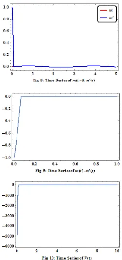
Figure 10 shows that the derivative of Lyapunov function (4.1) is less than or equal to zero for t is bigger than zero

(i.e. ( )

V t



≤

0 for

t

≥

0)

which strongly support that the synchronization is stable on the chosen sliding surfaces.

5. CHAOTIC SECURE COMMUNICATIONS

(8)

synchronization and to carry the message (Fig. 11). In the modulator the chaotic carrier signal

c t

( )

produced by the drive system is modulated by the message signal

m t

( )

to generate the transmitted signal

s t

( )

. Modulation is achieved by mixing the message signal with the chaotic carrier signal using a mixing algorithm which is simply a function of the message and chaotic carrier signals, i.e.

s t

( )

=

f m t c t

(

( ), ( )

)

.

In this paper the transmitter and the receiver are taken as TDCM and Rossler systems respectively. Let

s t

( )

be the transmitted signal that is the sum of the message signal

m t

( )

and the chaotic carrier signal

c t

( )

from the drive system. Here the message signal is chosen to be a periodic function

m t

( )

=

0.01sin 2

t

. With this choice the chaotic carrier signal

c t

( )

, chosen to be the state variable

x

₁ (representing number of tumour cells ) of the drive system. To recover the message the demodulator calculates the difference between the signal

s t

( )

from the modulator and

c t

′

( )

from the response system as

m t

′

( )

. The results (in Fig 7 and 8) show that when there is no synchronization between the drive and the response systems, the message signal

m t

( )

and the demodulated chaotic signal

m t

′

( )

are quite unrelated but when the controller is activated at

t

=

0.2

synchronization occurs after a short transient time and then the recovered and the original messages are identical. It is also confirmed by the convergence of the difference

( )

m t

′ −

m t

to zero shortly after the controller is activated (Fig 9) and that is because when the drive and response systems are completely synchronized

c t

′

( )

=

c t

( )

and consequently

m t

′

( )

=

m t

( )

.

6. CONCLUSIONS

In this computational study, the problem of practical synchronization of chaotic systems is done using RAMSC under the effects of the model uncertainties, external disturbances and unknown parameters in synchronizing the two different chaotic systems (TDCM & Rossler). Numerical simulations are presented to show the applicability and feasibility of the proposed study using Mathematica. We conclude three remarkable features of our proposed study that are:

(1) The implemented technique in our study was robust with respect to the model uncertainties, external disturbances and unknown parameters.

(2) It can be easily realized and implemented in real world applications without requiring the bounds of the model uncertainties, external disturbances and unknown parameters to be known in advance.

(9)

REFERENCES

1. W. Xiang, Y. Huangpu, Second-order terminal sliding mode controller for a class of chaotic systems with unmatched uncertainties. Commun Nonlinear Sci Numer Simulat, 15 (2010) 3241–3247.

2. M. Rafikov, J. M. Balthazar, On control and synchronization in chaotic and hyperchaotic systems via linear feedback control. Commun Nonlinear Sci Numer Simulat, 13 (2008) 1246–1255.

3. S. Bowong, Adaptive synchronization between two different chaotic dynamical systems. Commun Nonlinear Sci Numer Simulat, 12 (2007) 976–985.

4. H. Chen, G. Sheu, Y. Lin, C. Chen, Chaos synchronization between two different chaotic systems via nonlinear feedback control. Nonlinear Anal, 70 (2009) 4393–4401.

5. M.T. Yassen, Controlling, synchronization and tracking chaotic Liu system using active backstepping design.

Phys Lett A, 360 (2007) 582–587.

6. F. Wang, C. Liu, Synchronization of unified chaotic system based on passive control. Physica D, 225 (2007) 55–60.

7. Ahmad, I., Saaban, A., Ibrahim, A., Shahzad, M., 2014, “Global Chaos Identical and Nonidentical Synchronization of a New Chaotic System Using Linear Active Control,” Complexity, DOI: 10.1002/cplx.21573.

8. W. Chang, PID control for chaotic synchronization using particle swarm optimization. Chaos Soliton Fract, 39 (2009) 910–917.

9. Y. Sun, Chaos synchronization of uncertain Genesio–Tesi chaotic systems with dead zone nonlinearity. Phys Lett A, 373 (2009) 3273–3276.

10. F. Jianwen, H. Ling, X. Chen, F. Austin, W. Geng, Synchronizing the noise-perturbed Genesio chaotic system by sliding mode control. Commun Nonlinear Sci Numer Simulat, 15 (2010) 2546–2551.

11. M. Feki, Sliding mode control and synchronization of chaotic systems with parametric uncertainties. Chaos Soliton Fract, 41 (2009) 1390–1400.

12. C. Lin, Y. Peng, M. Lin, CMAC-based adaptive backstepping synchronization of uncertain chaotic systems.

Chaos Soliton Fract, 42 (2009) 981–988.

13. A. A. Ahmadi, V.J. Majd, Robust synchronization of a class of uncertain chaotic systems. Chaos Soliton Fract, 42 (2009) 1092–1096.

14. M. M. Asheghan, M.T.H. Beheshti, An LMI approach to robust synchronization of a class of chaotic systems with gain variations. Chaos Soliton Fract, 42 (2009) 1106–1111.

15. N. Cai, Y. Jing, S. Zhang, Modified projective synchronization of chaotic systems with disturbances via active sliding mode control. Commun Nonlinear Sci Numer Simulat, 15 (2010) 1613–1620.

16. H. Kebriaei, M.J. Yazdanpanah, Robust adaptive synchronization of different uncertain chaotic systems subject to input nonlinearity. Commun Nonlinear Sci Numer Simulat, 15 (2010) 430–441.

17. C. Chen, Quadratic optimal neural fuzzy control for synchronization of uncertain chaotic systems. Expert Syst Appl, 36 (2009) 11827–11835.

18. H. Wang, Z. Han, Q. Xie, W. Zhang, Finite-time chaos synchronization of unified chaotic system with uncertain parameters. Commun Nonlinear Sci Numer Simulat, 14 (2009) 2239–2247.

19. J. Ma, A. Zhang, Y. Xia, L. Zhang, Optimize design of adaptive synchronization controllers and parameter observers in different hyperchaotic systems. Appl Math Comput, 215 (2010) 3318–3326.

20. E. Hwang, C. Hyun, E. Kim, M. Park, Fuzzy model based adaptive synchronization of uncertain chaotic systems: robust tracking control approach. Phys Lett A, 373 (2009) 1935–1939.

21. H. Salarieh, M. Shahrokhi, Adaptive synchronization of two different chaotic systems with time varying unknown parameters. Chaos Soliton Fract, 37 (2008) 125–136.

22. M. P. Aghababa, A. Heydari: Chaos synchronization between two different chaotic systems with uncertainties, external disturbances, unknown parameters and input nonlinearities. Applied Mathematical Modelling, 36 (2012) 1639–1652.

23. M. P. Aghababa, M. E. Akbari: A chattering-free robust adaptive sliding mode controller for synchronization of two different chaotic systems with unknown uncertainties and external disturbances, Applied Mathematics

and Computation, 218 (2012) 5757–5768.

24. Khan, A., Shahzad, M., 2013, “Synchronization of circular restricted three body problem with Lorenz hyper chaotic system using a robust adaptive sliding mode controller,” Complexity18, 58–64.

25. Shahzad, M., 2015, “The Improved Results with Mathematica and Effects of External Uncertainty & Disturbances on Synchronization using a Robust Adaptive Sliding Mode Controller: A Comparative Study,”

Nonlinear Dynamics79, 2037-2054.

26. M. Pourmahmood, S. Khanmohammadi, G. Alizadeh, Synchronization of two different uncertain chaotic systems with unknown parameters using a robust adaptive sliding mode controller. Commun Nonlinear Sci

Numer Simulat, 16 (2011) 2853–2868.

(10)

29. Njah, A. N., 2011, “Synchronization via active control of parametrically and externally excited

Φ −

6 Van der Pol and Duffing oscillators and application to secure communications,” Journal of Vibration & Control17, 493-504.

30. Yang, T., 2004, ‘‘A survey of chaotic secure communication systems,’’ International Journal of Computational Cognition 2, 81–130.

31. Bu, S. and Wang, B. H., 2004, ‘‘Improving the security of chaotic encryption by using a simple modulating method,’’ Chaos, Solitons and Fractals 19, 919–924.

Source of support: Nil, Conflict of interest: None Declared