ANTHROPOGENIC CONTROLS ON OVERWASH DEPOSITION: EVIDENCE AND CONSEQUENCES
Laura J. Rogers
A thesis submitted to the faculty at the University of North Carolina at Chapel Hill in partial fulfillment of the requirements for the degree of Master of Science in the Department of
Geological Sciences.
Chapel Hill 2015
Approved by:
Laura J. Moore
Antonio B. Rodriguez
iii ABSTRACT
Laura J. Rogers: Anthropogenic Controls on Overwash Deposition: Evidence and Consequences (Under the direction of Laura J. Moore)
Accelerated sea-level rise and potential future increases in storminess due to climate
change will threaten the vitality of barrier islands by lowering their relative elevation and altering
overwash frequency. High-density development may further increase island vulnerability by
restricting delivery of overwash to the subaerial island. I analyzed pre- and post-Hurricane Sandy
(2012) LiDAR surveys of the New Jersey coast to assess human influence. I compared natural
environments to two developed environments (commercial and residential) using
shore-perpendicular topographic profiles. The volume of overwash delivered to residential and
commercial areas is reduced by 40% and 90%, respectively, of that delivered to the natural
environment. I use this analysis and an exploratory barrier island evolution model to assess
long-term impacts of anthropogenic structures. Simulations suggest natural barrier islands may persist
under a range of likely future sea-level rise scenarios (7–13 mm/yr) whereas developed barrier
iv
ACKNOWLEDGEMENTS
I would like to express my thanks to my thesis advisor, Dr. Laura J. Moore, my
committee, Drs. Tamlin Pavelsky and Antonio B. Rodriguez as well as Drs. Brad Murray and
Evan Goldstein for all their support, feedback and engagement throughout this learning process.
I must also thank the UNC Geological Sciences’ Martin Fund and the NSF Geomorphology and
Land Use Program (Grant #EAR 1053151) for their generous funding without which this work
v
TABLE OF CONTENTS
LIST OF TABLES………..…vi
LIST OF FIGURES………...vii
CHAPTER 1: ANTHROPOGENIC CONTROLS ON OVERWASH DEPOSITION ...1
Introduction………...………..……1
Storm statistics and study area ... ………...………...….4
Methods and results………...………...……….5
Overwash analysis ...………...……..………...………5
Calculation of overwash extent and volume………...……….…5
Error analysis and field comparisons………...………....….…7
Characteristics of overwash deposition………..…………...10
Distribution of overwash ………...………11
Long-term impacts on barrier island evolution………...…...…13
Discussion………...………..……14
Conclusion ………...……….…18
Tables and Figures………..…19
APPENDIX A. INTERPOLATION INDUCED ERROR ANALYSIS……….….………...32
APPENDIX B. FIELD OBSERVATIONS…….……….………..…33
vi
LIST OF TABLES
Table 1. LiDAR metadata………...……19
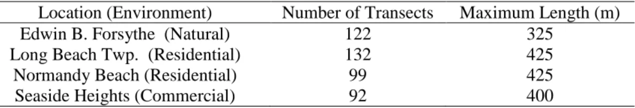
Table 2. Summary of number and length of transect by environment………...……19
Table 3. Overwash characteristics by environment………....…19
Table 4. Overwash relationship variables………..…....19
vii
LIST OF FIGURES
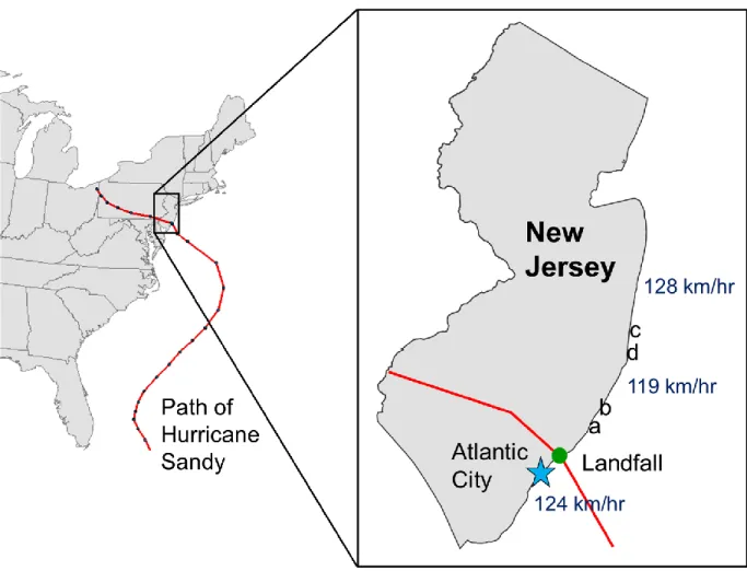
Figure 1. Path of Hurricane Sandy and relative study area locations………...………..21
Figure 2. Study area aerial images………..22
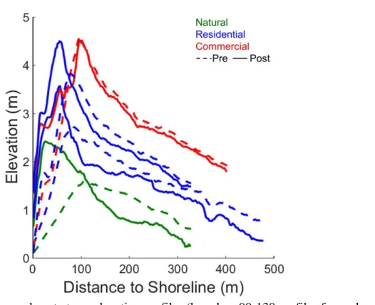
Figure 3. Pre and post-storm average elevation profiles……….23
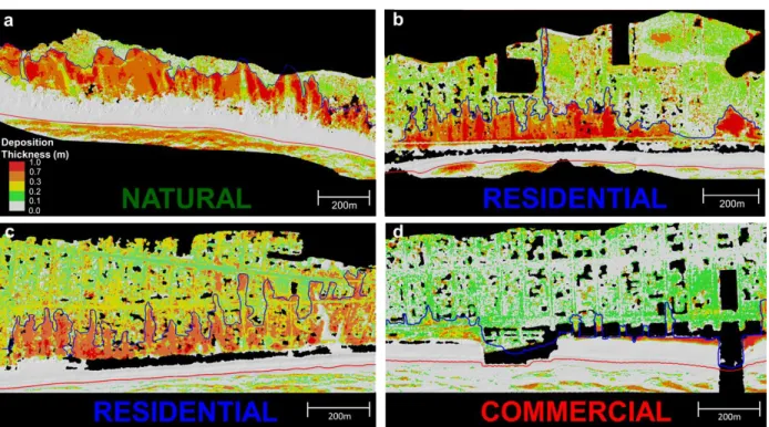
Figure 4. Elevation change models by environment………...………24
Figure 5. Annotated elevation change profile………..…...25
Figure 6. Average change profile………26
Figure 7. Overwash thickness comparison……….…27
Figure 8. Linear deposition of overwash……….……28
Figure 9. Overwash deposition distribution………29
Figure 10. Barrier island evolution modelling results……….………...……30
1
CHAPTER 1: ANTHROPOGENIC CONTROLS ON OVERWASH DEPOSITION
1. Introduction
Barrier islands are narrow, low-elevation landforms that are highly sensitive to changes
in sea level and storm activity. The population densities of barrier islands along the Atlantic and
Gulf coasts of the U.S. are, on average, three times greater than those of coastal states and are
increasing [Zhang and Leatherman, 2011]. Additionally, tourism is the largest business sector in the world and coastal tourism, including on barrier islands, is the greatest segment of that global
industry [Honey and Krantz, 2007].Much of the attraction to barrier islands stems from their natural beauty and abundance of recreational opportunities, a consequence of their low elevation,
typically only ~2 m above sea level [Psuty, 2002].
The same characteristics that make barrier islands popular places to live and visit also
make them especially vulnerable to changing environmental conditions. Conservative estimates
predict global sea level will rise between 28 and 61 cm by 2100 [Stocker et al., 2013]. Kopp et al. [2014] combine local SLR projections and IPCC representative concentration pathway (RCP) 8.5 projections to suggest a SLR of 0.7 – 1.3 m by the year 2100 in New York City, translating to
average rates of 7–13 mm/yr – substantially faster than the current rate of 4 mm/yr based on
monthly mean sea level data from 1911 to 2014 (NOAA, 2015). Recent work also suggests
climate change will increase the frequency of the most intense hurricanes and tropical storms
[e.g., Knutson et al., 2010 and Emanuel, 2013]. The cumulative impact of rising sea level and more frequent, more intense storms will influence the behavior of barrier islands in the future
2
In recent decades, significant progress has been made in understanding the geological
development of barrier islands and the important role of overwash in their evolution. Field-based
studies have captured measurements of overwash geometry, volume and spatial configuration
[e.g., Morton and Sallenger, 2003; Donnelly and Sallenger, 2007; Carruthers et al., 2013;
Williams, 2015; Shaw et al., 2015; Lazarus and Armstrong, 2015]. Deposition of overwash sediment can occur as a result of wave run-up exceeding the dune crest (classified as run-up
overwash) or as a result of the total water level (tides plus storm surge) exceeding the dune crest
(classified as inundation overwash) [Sallenger, 2000]. Run-up overwash typically produces overwash fans arising from confined flow, whereas inundation overwash generally results in
sheetwash deposits arising from laterally unconfined flow. Back-beach morphology, vegetation
and development also affect the shape and characteristics of overwash deposition [Donnelly et al., 2006]. Sallenger et al. [2001, 2003] and Stockdon et al. [2002, 2009] improved upon the
accuracy of ground-based methods by introducing the use of LiDAR to resolve beach-change
signals. Early work by White and Wang [2003] used small-scale LiDAR-derived DEMs to
determine spatial patterns of coastal volumetric change. They identified a statistically significant
difference in net volumetric change over a four year period in regions of the beach categorized as
developed, undeveloped or nourished. Additionally, tools have been developed to model and
predict erosion in response to the devastation caused by recent storms such as Hurricanes Katrina
and Sandy. These include, but are not limited to, process-based models of waves and sediment
transport [e.g., Roelvink et al., 2009; Palmsten and Holman, 2012] and statistical Bayesian modeling approaches [e.g., Plant and Stockdon, 2012].
Previous studies address the impacts of anthropogenic structures and development on
3
be quantified. Not only is the presence of human development on islands increasingly common,
but there is a strong coupling between the socioeconomic value placed on barrier islands and the
morphologic evolution of islands themselves [e.g., Werner and McNamara, 2007; McNamara and Werner, 2008a, 2008b; McNamara and Keeler, 2013; Jin et al., 2013; Lazarus, 2014].
Anthropogenic influence and associated feedbacks have long been recognized for their impact in
other natural systems. For example, anthropogenic modification of river systems interrupts the
hydrological cycle and causes magnified flood stages [Criss and Shock, 2001] overfishing of the world’s fish supply leads to loss of biodiversity [Jackson et al., 2001] and increases in wildfire
severity have been linked to fire prevention practices, which lead to excess fuel available for
burning [Schoennagel et al., 2004]. However, our understanding of the feedbacks associated with human alteration of barrier islands is in its early stages.
Because overwash supplies sediment to the subaerial island and is the mechanism by
which islands migrate landward and maintain elevation above sea level, loss or reduction of
sediment delivery to the island interior may ultimately lead to premature island narrowing and
drowning, a phenomenon recognized from numerical models of island behavior [Magliocca et al., 2011]. Many barrier island evolution models incorporate overwash flux as an adjustable parameter [e.g., Wolinsky and Murray, 2009; Lorenzo-Trueba and Ashton, 2014; and Walters et
al., 2014], however overwash flux is poorly constrained (especially as it relates to developed shorelines) and direct measurements of overwash deposition have yet to be used to parameterize
overwash flux in models of island evolution.
Here, using LiDAR-based surveys of topography collected before and after Hurricane
Sandy along a barrier island in New Jersey, USA, I quantify the impact of anthropogenic
4
area. I then use these results to parameterize a model of barrier island evolution (from Lorenzo-Trueba and Ashton, [2014]) to demonstrate the likely effect of anthropogenically generated
differences in overwash delivery on long-term barrier evolution.
2. Storm statistics and study area
Classified as a post-tropical cyclone, Hurricane Sandy made landfall northeast of Atlantic
City, New Jersey on 29 October 2012 [Blake et al., 2013]. Storm surge coupled with spring tides brought water levels to more than 1 m above average for a full day [NOAA, 2013] and led to
record-breaking high water levels throughout New Jersey. Maximum water levels reached 3.5
and 2.0 m MSL at The Battery, NY and Atlantic City, NJ, respectively [NOAA, 2013]. Maximum
sustained wind speeds of 130 km/hr with gusts up to 145 km/hr were recorded in New York and
New Jersey. The overall minimum central pressure reached 940 mb just hours prior to landfall.
Preliminary reports estimate that the storm caused nearly $50 billion in damage within the U.S.
[Blake et al., 2013].
I analyze overwash deposition in four areas within a 60 km alongshore reach north of
Sandy’s landfall, encompassing three categories of environments: 1) a natural environment,
which is relatively undisturbed by human influence; 2) a residential environment, defined as a
region of family-size homes built on piling foundations; and 3) a commercial environment,
typified by the presence of large commercial buildings built on slab foundations (Figures 1 and
2). A 1.2 km-long alongshore reach within the Edwin B. Forsyth Wildlife Refuge serves as the
“natural environment” study site. The “residential environment” consists of two regions for
comparison to reduce biases introduced as a result of the relative alongshore location of the
environments. The first is within Long Beach Township and the second is 50 km north at
5
environment”. The tidal range at all sites is 1.8 m [NOAA, 2013] with prevailing winds from the north-west. Average pre-storm profile elevation ranges from 2.5 m to 4.5 m across the
environments (Figure 3) and much of this variation is attributable to differences in development.
High water marks left by the storm at the north and south ends of my study area were within 0.25
m, at 2.65 m and 2.40 m (NAVD88; hereafter all elevations are reported relative to datum
NAVD88), respectively [McCallum et al., 2013] and maximum wind speeds across the study area were within a 10 km/hr range (Figure 1) [Blake et al., 2013]. The close proximity of my sites, the large size of this “super storm” relative to the length of my study area, and the
similarity of both high water mark elevations and wind speeds, allow me to assume that observed
differences in overwash extent and volume across the sites are likely to be largely a function of
differences in development rather than storm characteristics.
3. Methods and results
3.1 Overwash analysis
3.1.1 Calculation of overwash extent and volume
I quantify the impact of anthropogenic development on the delivery of overwash
sediment to the island interior by targeting two related parameters: 1) the landward extent of
overwash deposition; and 2) the volume of overwash sediment. For the purpose of this study, I
define the landward overwash extent as the distance in meters from the pre-storm mean high
water (MHW) shoreline to the landward-most reach of overwash deposition (measured
perpendicular to the shoreline). Volume of deposition is measured as the total quantity of
sediment deposited beyond the pre-storm dune crest. The pre-storm MHW shoreline is defined as
the 0.7 m contour line. I use LiDAR first-return surveys collected by the US Geological Survey
6
to measure variability in three dimensions. Point spacing and system error measurements are
summarized in Table 1.
To prepare both pre- and post-storm data sets I use an adaptive TIN densification
algorithm within ADPAT 1.0 (USGS developed software [Zhang and Cui, 2007]) to remove
buildings and vegetation; I use ortho-rectified aerial photos to verify that only bare-earth points
are retained. Quick Terrain Modeler grids both data sets to create pre- and post-storm surface
models using the dataset point spacing to define the underlying grid spacing and optimize
resolution. I difference the two surface models to create a pre- to post-storm elevation change
model (Figure 4). Using all three models, I then extract relevant parameters for quantification.
The pre-storm MHW shoreline serves as a baseline for measurements collected along cross-shore
transects (perpendicular to the shoreline) placed at 10 m alongshore intervals (Figure 5). The
number of transects measured and the cross-shore lengths of transects for each environment are
summarized in Table 2. Transects reaching into the back-barrier bay are truncated to reflect only
sub-aerial data.
To determine the landward extent of overwash deposition at each transect I use the
LiDAR-derived elevation-change model in combination with aerial imagery. The landward
extent of overwash deposition in the natural environment is easily manually digitized using
imagery by visually comparing the pre- and post-storm images to identify the seaward edge of
fresh overwash deposits. However, given that manually digitizing from aerial imagery in
developed areas is significantly more complex (because limited color contrast makes it difficult
to distinguish between overwash sand and pre-existing sand in driveways and yards) I use the
overwash extent digitized from imagery in the natural environment to develop a binary change
7
change model. I then apply this binary change scale to the respective LiDAR
elevation-change model so that I can clearly see and then manually digitize the landward overwash extent
in the residential and commercial areas. A modified use of the Digital Shoreline Analysis System
(DSAS [Thieler et al., 2009] calculates the distance from the shoreline to the maximum extent of
overwash deposition along each transect. For ease of comparison, I represent overwash extent
both dimensionally (𝐸𝑜𝑤 ; absolute extent of overwash in meters) and in a non-dimensionalized
form:
𝐸𝑜𝑤∗ = 𝐸𝑊𝑜𝑤
𝐵𝐼 Equation (1)
where 𝐸𝑜𝑤∗ is non-dimensionalized extent of overwash and 𝑊
𝐵𝐼 is initial cross-shore width of the
barrier island in meters.
To calculate the volume of overwash deposition along each transect, I compute the area
under the elevation-change profile and represent these volumes as width-averaged quantities in
units of m3/m. The point at which deposition begins is defined as the location where the
elevation change becomes positive; deposition ends at the limit of extent of overwash deposition
(Figure 5). I define characteristic overwash deposition geometries for each environment by
averaging profiles across each study area (Figure 6).
3.1.2 Error analysis and field comparisons
Error in LiDAR data is attributed to a combination of four components: system
measurement error, interpolation, horizontal displacement and survey error [Hodgson and
Bresnahan, 2004]. Sallenger et al. [2003] found they could resolve beach-change signals in LiDAR surveys with a vertical precision of ±15 cm. However, when detecting change across
8
address [Zhang et al., 2005]. Thus, I compare 20 control points between the pre- and post-storm first-return surveys to determine if relative offset error is a factor. I use building corners for most
of my control points, as they are easily identifiable and unlikely to be altered by the storm. Direct
comparison of the control points for each survey yields an R2 correlation of 0.99 with an absolute
mean error of less than 5 cm. I therefore consider relative offset error to be negligible.
To quantify errors associated with interpolation I removed 1000 points prior to
interpolation for comparison to post-interpolation points. The resulting ~5 cm of vertical error is
likely an overestimate as removing 1000 points from the data series increases the distance
between points (thereby introducing error). Further error analysis is found in Supplemental
Information (SI) A.
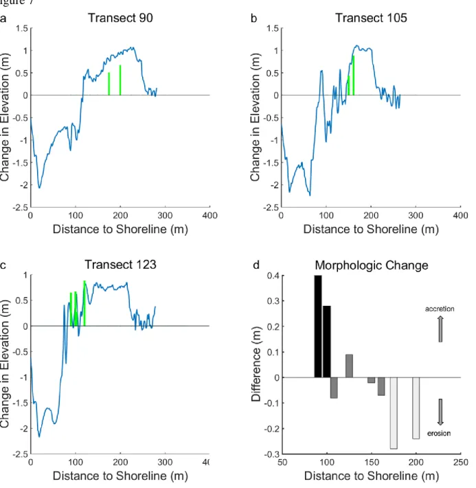
To test error estimates and the morphologic change signal, I collected eight slide-hammer
Geoprobe cores (in November, 2014) along three transects at designated distances from the
MHW shoreline. Cores were collected in my natural area study site where overwash deposits
were unlikely to have been disturbed by anthropogenic influences following Hurricane Sandy.
Detailed core logs and grain-size analyses are presented in SI B. I measured overwash thickness
in the cores as the distance between the ground surface and the first major lithologic contact
(typically the contact between medium to coarse sand [overwash] and underlying peat).
Comparison of overwash thickness measured in cores versus thicknesses derived from LiDAR
observations yields absolute differences ranging from 2 to 40 cm, with an average absolute
difference of 18 cm (Figure 7).
The signs of the differences follow expected patterns of morphologic change associated
with nearshore beach recovery and landward deflation due to aeolian transport and vegetation
9
thus not only include errors arising from the LiDAR analysis but also volumetric changes in
overwash deposits that have occurred since deposition. For example, the two cores in which I
measured overwash thicknesses of -28 and -24 cm relative to those derived from LiDAR are
farthest from the shoreline, have limited vegetation due to overwash burial and are therefore
vulnerable to erosion by wind. Additionally, the ground surface in these areas exhibited signs of
deflation at the time of core collection; moreover, < 1m2 plots of land surrounding proximal
vegetation clearly had amassed aeolian sediment. Consequently, significant aeolian reworking
had occurred in the exposed, landward-most sections in the two years since Hurricane Sandy.
Thus, this process of aeolian reworking and deflation reduced overwash thicknesses measured in
these locations relative to the thicknesses measured using LiDAR observations.
I found similar post-storm morphologic changes documented on the seaward side of the
island. The two cores I collected closest to the shoreline came from a zone in which recent
accretion was apparent, likely via onshore ridge-and-runnel migration of bars. This resulted in
field estimates of overwash deposition thickness substantially larger than those derived from the
LiDAR analysis. These cores were also collected within a zone where the LiDAR analysis
indicates alternation between erosional and accretional areas in close proximity, suggesting that
positional error may also be affecting the accuracy with which comparison can be made at these
cross-shore locations.
Given the likelihood that accretion and erosion have affected preservation of the
overwash signal and that the direction of the differences between remote and field-based
measurements are as expected based on likely morphological changes since the storm occurred, I
conclude that the LiDAR analysis is likely producing depths that are a reasonable reflection of
10
Thus, the average 18 cm difference between the core and LiDAR analysis, if taken to represent
the uncertainty in my measurements of overwash deposit thickness from LiDAR observations, is
most likely a substantial overestimate of actual uncertainty. Moreover, the average difference is
also only 3 cm greater than the 15 cm of error identified as sufficient to resolve changes in
morphology by Sallenger et al., [2003]. These findings suggest that the LiDAR analysis is providing a reasonably accurate representation of morphologic change caused by Hurricane
Sandy.
3.1.3 Characteristics of overwash deposition
Prior to Hurricane Sandy, the dune crest in the natural area reached an average elevation
of 2.5 m and was located approximately 20 m landward of the shoreline. Vegetation consisted of
mature dune grasses backed by marsh and previous overwash deposits are clearly visible in
pre-storm satellite imagery. To ensure that only the extents of newly deposited overwash fans were
analyzed, I completed a pre- and post-storm image comparison.
Dunes in the natural environment were uniformly reduced by 1 m in elevation during
Hurricane Sandy. Visual inspection of aerial images indicates deposition consistent with laterally
unconfined flow. Landward overwash extent ranged from 188 to 309 meters (average = 252 m)
and reached the back-barrier bay in 28% of profiles. The volume deposited ranged from 23 to
125 m3/m (Figures 8 and 9, Table 3). Volume of sediment deposited into the back-barrier bay,
however, is not captured in measurements, leading to a likely under-prediction of both landward
overwash extent and volume of deposition in the natural environment.
In the residential area, pre-storm dune crests averaged 3.5 – 4.5 m in elevation at both
sites (not counting breaks in the dunes associated with beach access). Most dunes were reduced
11
indicates overwash was channelized. These areas of confined flow correspond to locations where
overwash penetration was greatest. The average landward overwash extent in the residential
environments is 169 meters and volumes range from 2 to 117 m3/m (Figures 8 and 9, Table 3).
Likely because a distinct dune line was absent in the commercial area, catastrophic
damage to beachfront infrastructure occurred during the storm. The boardwalk is 4.5 m in
elevation and 75–100 meters from the shoreline. Regions of confined flow occurred along this
section of beach, but were less common than in the residential area (fewer channels per
kilometer). The average landward extent of overwash deposition in the commercial environments
was 111 meters and overwash volume ranges from 0 to 35 m3/m, (Figures 8 and 9, Table 3).
3.1.4 Distribution of overwash
Where overwash flow was uninhibited by anthropogenic structures (i.e. in the natural
environment) no signs of channelized flow were visible, whereas channelized, confined
overwash events were prevalent in the residential and commercial environments. Combining
measurements from all environments, I compared the landward overwash extent and volume of
deposition (𝑅2 = 0.68, 𝑝 < 0.01) (Figure 8a). The resulting statistically significant linear
relationship can be described as:
𝑉𝑜𝑤 = 𝐾 × 𝐸𝑜𝑤− 𝐴 Equation (2)
where 𝑉𝑜𝑤 is volume of overwash, K is a coefficient and A is a constant which accounts for offset
between the shoreline and the cross-shore location where overwash begins. When I repeat the
same analysis for each environment, the relationships remains linear and statistically significant
12
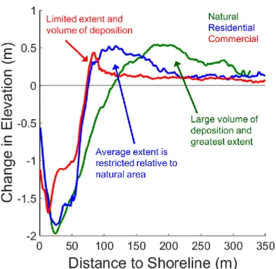
When anthropogenic factors are introduced, both the volume and landward extent of
overwash deposition decrease with increasing waterfront development. The average volume of
sediment delivered to the residential and commercial environments is reduced to just 60% and
10% of that delivered to the natural environment, respectively. Similarly, the average extent of
overwash in the natural environment was more than 2.25 times greater than in the commercial
environment. The range of values for both extent and volume (Figure 9) was greatest for the
residential environment (shown in both dimensional and non-dimensional terms). Only in the
natural environment did overwash extend into the back-barrier bay, (i.e., extent >1 in
non-dimensionalized terms, Figure 9c).
I can additionally consider the mass balance for each environment. An important
consideration here is that my measurements of the system are not closed because topographic
LiDAR data limits the analysis to the subaerial landscape. I calculated the mass balance as the
difference between the total volume of sand deposited by overwash and the total volume of
subaerial sand eroded, as measured from the shoreline to the bay within an environment. Though
sand delivered to, and captured by, the bay in the natural environment could not be accounted
for, and although the patterns of deposition were most different between the natural and
commercial environments, the mass balance in these two environments was similar: their
volumes were within 15% of each other, at an average sand loss of 5.3 m3/m and 4.6 m3/m for
the natural and commercial environments, respectively. By comparison, the residential area lost
an average of 2.9 m3/m of sand, although this number is likely artificially low because I was
unable to account for large amounts of sand eroded from beneath the piling foundations of the
many homes located within the zone of erosion (Figure 4), a phenomenon observed in post-storm
13
The results of my analysis suggest the following scaling relationships for the volume and
extent of overwash deposition as a function of the type of anthropogenic structures present
(assuming similar bathymetry and back-barrier elevation), for future use in analytic and
exploratory models of barrier island processes:
Equation (3):
Natural Residential Commercial
Volume 𝑉𝑜𝑤,𝑁= 𝑉𝑜𝑤,𝑁 𝑉𝑜𝑤,𝑅 = 0.6 × 𝑉𝑜𝑤,𝑁 𝑉𝑜𝑤,𝐶= 0.1 × 𝑉𝑜𝑤,𝑁
Landward Extent (m) 𝐸𝑜𝑤,𝑁= 𝐸𝑜𝑤,𝑁 𝐸𝑜𝑤,𝑅 = 0.7 × 𝐸𝑜𝑤,𝑁 𝐸𝑜𝑤,𝐶= 0.4 × 𝐸𝑜𝑤,𝑁
3.2 Long-term impacts on barrier island evolution
I use an exploratory morphodynamic barrier island evolution model, introduced by
Lorenzo-Trueba and Ashton [2014], to investigate modes of island behavior under a variety of
conditions. This model considers a barrier island cross-section through an idealized geometric
configuration and uses a system of equations to determine long-term (decades to centuries to
millennia) island tendencies. Three change components (passive flooding due to sea-level rise,
shoreface fluxes, and overwash) determine the evolution of the barrier system, which is fully
resolved by the shoreline toe, the shoreline, the back-barrier, the barrier height, and the rate of
change of the back-barrier height. This system of equations is numerically solved to examine
coupled, non-steady-state behaviors that include dynamic equilibrium, height drowning, and
width drowning. Height drowning in this model occurs when sediment fluxes due to overwash
are insufficient to maintain island elevation relative to rising sea level. Width drowning occurs
when sediment flux to the back-barrier is insufficient to maintain island geometry during
14
I use this model to investigate the long-term impact of decreases in overwash delivery on
island evolution caused by development. To provide context for considering implications across
barrier island systems broadly, I apply generic island characteristics similar to those used by
Lorenzo-Trueba and Ashton [2014], (Table 5), in conjunction with the empirically derived
scaling relationships for overwash flux (𝑄𝑜𝑤,𝑚𝑎𝑥) I present at the end of Section 3.1.4.
Lorenzo-Trueba and Ashton [2014] capture impacts of storm frequency and magnitude as well as
potential anthropogenic effects in a single term, 𝑄𝑜𝑤,𝑚𝑎𝑥, which represents the maximum annual
volume of overwash delivered by all storms, and they explore values from 0-100 m3/m/yr. For
consistency with this previous work, I set 𝑄𝑜𝑤,𝑚𝑎𝑥 to 30 m3/m/yr for the natural environment (set
this in context with my calculations, this is equal to 50% of the volume of overwash deposition I
calculated for this environment). I then applied Equation 3, yielding scaled 𝑄𝑜𝑤,𝑚𝑎𝑥 values of 18
and 3 m3/m/yr for the residential and commercial environments, respectively. Simulations
suggest that decreasing overwash flux to the back-barrier shifts the long-term tendency of the
island from dynamic equilibrium to width drowning in the residential environment and to height
drowning in the commercial environment at significantly high rates of SLR (> 5 mm/yr) and
deeper back-barrier depths (> 5 m) (Figure 10). It should be noted Figure 10c represents a
worse-case scenario illustrating that the risk of drowning is greatly increased as the rate of SLR
increases and as the depth of the back-barrier bay increases. For comparison, the average depths
of Barnegat Bay (NJ, USA), Pamlico Sound (NC, USA) and the Chesapeake Bay (MD/VA,
USA) are 1, 2 and 6 meters, respectively [Miselis et al., 2013 and Urquhart et al., 2013].
4. Discussion
The volumes and landward extents of overwash deposition measured in this study are 0–
15
environments and fall within the expected range based on previous estimates. Carruthers et al. [2013] compile 30 estimates of overwash fan geometric properties from a number of studies and
report landward overwash extents of 13–359 m and volumes of 8–190 m3/m, respectively.
Additionally, the average volume of 62 m3/m calculated for my “natural environment” is well in
line with that estimated for overwash associated with the Hurricane of 1938 on Long Island, NY
of ~54-80 m3/m [Redfield and Miller, 1957], an environment broadly similar to that studied here.
My results extend previous work on overwash by demonstrating a linear relationship
between overwash extent and volume (Figure 8). Furthermore, my findings demonstrate that as
the landward extent of overwash deposition increases, the relationship with overwash volume
becomes less tightly constrained and the range of overwash volumes for any given landward
overwash extent increases. This latter phenomena is likely the result of progressive increases in
lateral spreading and infiltration which occur as the landward overwash extent increases, a
process described in detail by Donnelly et al., [2009].
Similar to previous studies, which cite beach access points and roads as likely conduits
for channelized overwash deposition [e.g., Hall and Halsey, 1991; Nordstrom, 1994; Houser, 2013], I find a greater frequency of channelized deposits in the residential and commercial
environments relative to the natural environment. Analysis of aerial imagery suggests that
locations of channelized flow within the developed environments in my study correspond to
roads and beach access points. This indicates that infrastructure (i.e., roads, parking lots, etc.)
and building placement can control overwash deposition. Further, I found pre-storm dune height
to be weakly correlated with overwash extent and volume (𝑅2 = 0.38 and 𝑅2 = 0.30,
respectively) yet statistically significant (𝑝 < 0.01) (Figure 11). Although a weak, yet
16
deposition, dune height is not strongly predictive of overwash deposition in this case, likely
because dune erosion was so extreme as a result of the high intensity and long duration of
Hurricane Sandy. This lack of correlation with pre-existing beach morphology further signifies
the role of anthropogenic influence on deposition of overwash.
The volume of overwash deposition varied according to the type of environment,
decreasing to 60% and 10% of that delivered to the natural area in the residential and commercial
environments, respectively. Because much of the deposition occurring in the developed
environments amassed in roads as channelized deposition, the relative volumes measured in this
study should be considered upper bounds on deposition; humans will undoubtedly move sand
back to the beach (i.e., bulldoze to clear roads) during clean-up (in my study I used post-storm
surveys collected prior to clean-up). Additionally, sand delivered to the back-barrier bay in the
natural environment was not captured due to limitations of topographic (in contrast to
bathymetric) LiDAR. These factors imply the spread between the amount of overwash sediment
delivered to the natural and developed environments is likely even greater than my calculations
suggest.
The most dramatic reduction in overwash occurred in the commercial area where, despite
the record high water levels produced by Hurricane Sandy, overwash extent was limited to the
area seaward of the boardwalk along nearly 50% of transects. This suggests that, in the presence
of buildings having a substantial alongshore extent, even major storms are unable to supply
overwash sediment to the island interior. From this we can infer that smaller, more frequent
storms are also unable to supply sediment to the interior of the island, thereby implying that
17
Previous modeling studies [McNamara and Werner, 2008a; Magliocca et al., 2011] warn of the long-term consequences of filtering high-frequency overwash events arising from
protection of infrastructure in the short-term (for example, by building a seawall or large
artificial dunes), which may lead to barrier narrowing and drowning. Similar filtering of
high-frequency events by anthropogenic manipulation is a recognized phenomenon with major
consequences in other geomorphic systems such as major rivers and forested areas [e.g., Criss and Shock, 2001; Schoennagel et al., 2004]. Ultimately, the filtering of smaller events has
historically led to more extreme, more costly events as demonstrated by river discharge
management, wildfire prevention and as predicted in coastal economic models by McNamara
and Werner [2008a].
My observational and modeling results suggest that increases in the density and extent of
development along barrier island coastlines will reduce overwash delivery, maintaining low
barrier islands even as sea levels rise, ultimately leading to increases in damage to infrastructure
and higher costs of recovery following large, overwash-producing events. My model results also
highlight the potentially catastrophic consequences of high-frequency filtering as it relates to the
persistence of barrier islands—they suggest that developed barrier islands will tend toward
drowning in the long term under anticipated accelerated SLR, whereas natural barriers will be
more likely to persist by means of landward migration via frequent overwash. Thus, we can
likely expect filtering of high-frequency—and partial filtering of the low-frequency—delivery of
overwash to ultimately impact not only barrier island evolution, but also coastal management
decision-making and policy (e.g., cost of insurance). Further work exploring the effects of
back-barrier bay depth (i.e., accommodation), interactions between back-barriers and back-back-barrier marshes
18
2008] on island response to decreased overwash delivery, as well as the potentially compounding
effects of offshore bars and beach slope on alongshore variation in water level [Cohn et al.,
2014] would potentially broaden the results found here.
5. Conclusions
I analyzed two key parameters – volume of overwash deposition and landward extent of
overwash deposition – to quantify anthropogenic controls on the delivery of overwash sediment.
By categorizing the section of the New Jersey shoreline immediately north of where Hurricane
Sandy made landfall into three distinct environments – natural, residential and commercial – I
was able to directly compare overwash characteristics under similar storm and initial
morphologic conditions. The volume of deposition in the residential and commercial
environments scaled to 60% and 10%, respectively, of the volume deposited in the natural
environment volume. This translates into a reduction of overwash delivery by 40% in the
residential areas and 90% in the commercial area. The landward extent of overwash was also
substantially reduced with increasing shoreline development: in the commercial area, overwash
was completely obstructed along 50% of the alongshore reach. This finding suggests that large
anthropogenic structures are highly effective at filtering overwash events.
The scaling relationships offered here provide a solid empirical foundation that can be
used to parameterize overwash delivery when modeling barrier island evolution in the presence
of infrastructure. Model results suggest that anthropogenic reductions in the flux of overwash
sediment reaching island interiors may ultimately lead to island drowning. Although Hurricane
Sandy was an extreme, low frequency event, it serves as a good example of the depositional
impacts that can be expected in the future with rising sea levels and the increased frequency of
19 6. Tables and Figures
Table 1. LiDAR metadata
Location: Storm: Collected by: Collection Date: Vertical/Horizontal Accuracy: Point Spacing: Ocean County, NJ Hurricane Sandy – Before USGS –
EAARL-B 26 Oct 12 20 cm/1 m 0.5 – 1.6m Hurricane Sandy
– After
USGS –
EAARL-B 01-05 Nov 12 20 cm/1 m 0.5 – 1.6m
Table 2. Summary of number and length of transect by environment
Location (Environment) Number of Transects Maximum Length (m)
Edwin B. Forsythe (Natural) 122 325
Long Beach Twp. (Residential) 132 425
Normandy Beach (Residential) 99 425
Seaside Heights (Commercial) 92 400
Table 3. Overwash characteristics by environment
Table 4.Overwash relationship variablesa
aK – relationship coefficient, A – shoreline to overwash offset constant
Environment # of Transects
𝐸𝑂𝑊 Range
(m)
Avg. 𝐸𝑂𝑊
(m)
Avg. 𝐸𝑂𝑊∗ 𝑉𝑂𝑊 Range
(m3/m)
Avg. 𝑉𝑂𝑊
(m3/m)
Natural 122 188 – 309 252.2 0.85 23.3 – 125.7 62.2
Residential 231 103 – 271 169.0 0.47 2.1 – 116.7 38.1
Commercial 92 25 – 203 108.1 0.27 0 – 35.1 7.7
Environment K A
Combined 0.36 -26
Natural 0.40 -39
Residential 0.39 -27
20 Table 5. Input parameters used in Figure 10
Parameter Symbol Units Value
Shoreface Response Rate K m3/m/y 10,000
Equilibrium Shoreface Slope α - 0.02
Shoreface Toe Depth Dt m 10
Equilibrium Island Width W m 300
Equilibrium Island Height H m 2
Back Barrier Bay Depth Db m 2, 5, 9
Sea Level Rise z mm/yr 0 – 15
21 Figure 1
22 Figure 2
23 Figure 3
24 Figure 4
25 Figure 5
26 Figure 6
27 Figure 7
28 Figure 8
29 Figure 9
Figure 9. Distribution of (a) overwash volume (b) landward extent of overwash and (c) non-dimensionalized extent of overwash. The natural environment allows the greatest volume and extent of overwash deposition while the
30 Figure 10
Figure 10. Phase diagrams illustrating the impact of anthropogenic development on barrier island evolution for different rates of sea-level rise, maximum overwash flux and back-barrier depths of (a) 2m, (b) 5m, and (c) 9m. Red and blue lines denote maximum overwash flux (𝑄𝑜𝑤,𝑚𝑎𝑥) for commercial and residential environments, respectively, scaled relative to a natural environment
31 Figure 11
32
APPENDIX A: INTERPOLATION INDUCED ERROR ANALYSIS Triangulation methods are sensitive to the position of data points and the removal of
points (as described in Section 3.1.2). Because the removal of points to assess accuracy results
in increases in local point spacing, point removal to quantify induced error due to triangulation
likely provides an overestimate of actual error. QT Modeler’s RMSE calculation provide an
additional measure of error introduced by interpolation. After the gridding process is complete,
QT Modeler calculates the RMSE of each 1 m grid square by comparing the original point cloud
to the gridded surface without the actual removal of points. This resulted in a similar, yet
33
APPENDIX B. FIELD OBSERVATIONS
In order to compare the remotely-sensed LiDAR observations analyzed for this study
with field observations, I collected cores and grab samples of surficial sediment from the Edwin
B. Forsythe Wildlife Refuge, Holgate, New Jersey. Field sampling was done November 15-16,
2014, approximately two years after the LiDAR survey was completed November 1-5, 2012.
The tidal range in this area is 1.8 m [NOAA, 2012] with prevailing winds from the north-west. Prior to the storm, dunes in this area averaged 2.5 m in elevation, located, on average, 20 m
from the shoreline. Vegetation consisted of mature dune grasses backed by marsh. Hurricane
Sandy delivered large amounts of overwash to the region. The original dune line was reduced by
1 m or more and vegetation was buried or removed by the storm.
Within the area of interest, I selected eight cross-shore transects for sampling (Figure
B.1). I collected nine slide-hammer Geoprobe sediment cores samples (Figure B.2), at designated
locations. Sample locations were selected based on ground-penetrating radar (GPR) profiles
collected concurrently using a Mala ProX with both 250 MHz and 500 MHz antennas. Cores
were collected in 6 cm diameter polycarbonate liners within a stainless steel core barrel (Figure
B.2). Cores ranged from 65 cm to 175 cm in depth. Additionally, hand auger cores were
collected at 25 m intervals along each of the eight transects with the intention to visually identify
overwash layers in the field.
Cores were opened, described, photographed, and sampled at the University of North
Carolina, Chapel Hill. Three representative cores are shown here (Figures B.3 – B.5). Based on
visual inspection and with the intention to compare down-core changes in grain size with the
extent of overwash, I selected three cores for detailed grain size analysis: BH123-2-2, BH105-5
34
(Figure B.6). I collected samples for grain size analysis at 15 cm intervals. Each sample was
exposed to 600⁰ C temperatures to remove organics, then analyzed using a Beckman Coulter LS
3 Series Laser Diffraction Particle Size Analyzer. The Wentworth scale was used to define
general grain size classes. Given the large sampling interval of 15 cm, the overwash depths
identified visually as described in Section 3.1.2 are generally comparable to overwash depths
identified using grain size analysis.
Comparison of overwash depths measured using LiDAR data with overwash depths
measured in the sediment cores reveals general similarities but indicates that (as expected)
changes have occurred due to natural beach processes in the intervening two years. I consider all
cores in my comparison, except for core BH-105-4-2, which was accidentally collected below
the depth of the base of the overwash signal I was attempting to capture (the overwash layer was
estimated, based on LiDAR analysis, to begin at a depth of 49 cm, but I augered to a depth of 78
cm before collecting my core sample). The resulting absolute range of difference between the
LiDAR analysis and the overwash thickness identified in my cores was 2 to 40 cm with an
average absolute difference of 18 cm (Table B1, Figure 5). As explained in Section 3.2, the sign
of the differences is reflective of the patterns of morphological diagenesis associated with
recovery (close to shore) and deflation (toward the back of the island) in the two years between
35
Table B.1. Sediment core locations and overwash depth comparisons
Core Dist. to Shore (m)
Northing Easting Overwash
Depth in Core (cm)
Overwash Depth from
LiDAR (cm) Diff. (cm)
90-6 175 4375769.32 562732.7499 50 78 -28
90-7 200 4375779.85 562714.5323 67 91 -24
105-4-2 133 4375635.87 562667.5412 126 49 -
105-5 150 4375640.61 562661.2974 43 45 -2
105-5-2 161 4375649.33 562653.2076 88 95 -7
123-2-2 90 4375468.65 562592.7106 65 25 +40
123-3 100 4375474.94 562585.7235 67 49 +28
123-3-2 103 4375476.04 562583.4492 27 35 -8
36 Figure B.1
37 Figure B.2
38 Figure B.3
39 Figure B.4
40 Figure B.5
41 Figure B.6
42
REFERENCES
Blake, E. S., Kimberlain, T. B., Berg, R. J., Cangialosi, J. P., & Beven II, J. L. (2013). Tropical Cyclone Report: Hurricane Sandy. National Hurricane Center,12, 1-10.
Carruthers, E. A., Lane, D. P., Evans, R. L., Donnelly, J. P., & Ashton, A. D. (2013). Quantifying overwash flux in barrier systems: An example from Martha's Vineyard, Massachusetts, USA. Marine Geology, 343, 15-28, doi:10.1016/j.margeo.2013.05.013. Cohn, N., Ruggiero, P., Ortiz, J., & Walstra, D. J. (2014). Investigating the role of complex
sandbar morphology on nearshore hydrodynamics. Journal of Coastal Research, SI(70), 53-58, doi: 10.2112/SI65-010.1.
Criss, R. E., & Shock, E. L. (2001). Flood enhancement through flood control. Geology, 29(10), 875-878, doi: 10.1130/0091-7613(2001)029<0875:FETFC>2.0.CO;2.
Donnelly, C., Kraus, N., & Larson, M. (2006). State of knowledge on measurement and modeling of coastal overwash. Journal of Coastal Research, 22(4), 965-991,
doi:10.2112/04-0431.1.
Donnelly, C., & Sallenger, A. H. (2007). Characterization and modeling of washover fans.
Proceedings of Coastal Sediments’ 07, 2061-2073, doi: 10.1061/40926(239)162.
Donnelly, C., Hanson, H., & Larson, M. (2009). A numerical model of coastal overwash. Proceedings of the ICE-Maritime Engineering, 162(3), 105-114, doi:
10.1680/maen.2009.162.3.105.
Duran-Vinent, O., & Moore, L. J. (2015). Barrier island bistability induced by biophysical interactions. Nature Climate Change, 5(2), 158-162, doi: 10.1038/NCLIMATE2474.
Emanuel, K. A. (2013). Downscaling CMIP5 climate models shows increased tropical cyclone activity over the 21st century. Proceedings of the National Academy of Sciences, 110(30), 12219-12224, doi: 10.1073/pnas.1301293110.
FitzGerald, D. M., Fenster, M. S., Argow, B. A., & Buynevich, I. V. (2008). Coastal impacts due to sea-level rise. Annu. Rev. Earth Planet. Sci., 36, 601-647.
Hall, M. J., & Halsey, S. D. (1991). Comparison of Overwash Penetration from Hurricane Hugo and Pre-Storm Erosion Rates for Myrtle Beach and North Myrtle Beach, South Carolina, USA. Journal of Coastal Research, 229-235.
Hodgson, M. E., & Bresnahan, P. (2004). Accuracy of Airborne Lidar-Derived Elevation.
Photogrammetric Engineering & Remote Sensing, 70(3), 331-339.
43
Houser, C. (2013). Alongshore variation in the morphology of coastal dunes: Implications for storm response. Geomorphology, 199, 48-61, doi: 10.1016/j.geomorph.2012.10.035.
Jackson, J. B., Kirby, M. X., Berger, W. H., Bjorndal, K. A., Botsford, L. W., Bourque, B. J., ... & Warner, R. R. (2001). Historical overfishing and the recent collapse of coastal
ecosystems. Science, 293(5530), 629-637, doi: 10.1126/science.1059199.
Jin, D., Ashton, A. D., & Hoagland, P. (2013). Optimal responses to shoreline changes: an integrated economic and geological model with application to curved coasts. Natural Resource Modeling, 26(4), 572-604, doi: 10.1111/nrm.12014.
Knutson, T. R., McBride, J. L., Chan, J., Emanuel, K., Holland, G., Landsea, C., ... & Sugi, M. (2010). Tropical cyclones and climate change. Nature Geoscience, 3(3), 157-163. doi:
10.1038/ngeo779.
Kopp, R. E., Horton, R. M., Little, C. M., Mitrovica, J. X., Oppenheimer, M., Rasmussen, D. J., ... & Tebaldi, C. (2014). Probabilistic 21st and 22nd century sea‐level projections at a global network of tide‐gauge sites. Earth's Future, 2(8), 383-406.,
doi: 10.1002/2014EF000239.
Lazarus, E. D. (2014). Threshold effects of hazard mitigation in coastal human–environmental systems. Earth Surface Dynamics, 2(1), 35-45, doi:10.5194/esurf-2-35-2014.
Lazarus, E. D., & Armstrong, S. (2015). Self-organized pattern formation in coastal barrier washover deposits. Geology, 43(4), 363-366, doi: 10.1130/G36329.1.
Leatherman, S. P. (1983). Barrier dynamics and landward migration with Holocene sea-level rise. Nature, 301, 15-17, doi: 10.1038/301415a0.
Lorenzo‐Trueba, J., & Ashton, A. D. (2014). Rollover, drowning, and discontinuous retreat: Distinct modes of barrier response to sea‐level rise arising from a simple morphodynamic model. Journal of Geophysical Research: Earth Surface, 119(4), 779-801,
doi: 10.1002/2013JF002941.
Magliocca, N. R., McNamara, D. E., & Murray, A. B. (2011). Long-term, large-scale
morphodynamic effects of artificial dune construction along a barrier island coastline.
Journal of Coastal Research, 27(5), 918-930, doi: 10.2112/jcoastres-d-10- 00088.1.
McCallum, B. E., Wicklein, S. M., Reiser, R. G., Busciolano, R., Morrison, J., Verdi, R. J., ... & Gotvald, A. J. (2013). Monitoring storm tide and flooding from Hurricane Sandy along the Atlantic coast of the United States, October 2012 (No. 2013-1043, pp. 1-42). US Geological Survey.
McNamara, D. E., & Keeler, A. (2013). A coupled physical and economic model of the response of coastal real estate to climate risk. Nature Climate Change, 3(6), 559-562,
44
McNamara, D. E., & Werner, B. T. (2008a). Coupled barrier island–resort model: 1. Emergent instabilities induced by strong human‐landscape interactions. Journal of Geophysical Research: Earth Surface (2003–2012), 113(F1), doi: 10.1029/2007JF000840.
McNamara, D. E., & Werner, B. T. (2008b). Coupled barrier island–resort model: 2. Tests and predictions along Ocean City and Assateague Island National Seashore, Maryland.
Journal of Geophysical Research: Earth Surface (2003–2012), 113(F1), doi: 10.1029/2007JF000841.
Miselis, J., Andrews, B., Ganju, N., Navoy, A., Nicholson, R., & Defne, Z. (2013) Mapping, Measuring, and Modeling to Understand Water-Quality Dynamics in Barnegat Bay-Little Egg Harbor Estuary, New Jersey. Sound Waves. 2013(2). Retrieved from
http://soundwaves.usgs.gov/2013/02/.
Morton, R. A., & Sallenger Jr, A. H. (2003). Morphological impacts of extreme storms on sandy beaches and barriers. Journal of Coastal Research, 560-573.
National Oceanic and Atmospheric Administration. (2013). NOAA Water Level and Meteorological Data Report: Hurricane Sandy. Retrieved from
www.tidesandcurrents.noaa.gov/publications/Hurricane_Sandy_2012_Water_Level_and_ Meteorological_Data_Report.pdf
National Oceanic and Atmospheric Administration. (2015). NOAA Tides and Currents. Retrieved from http://tidesandcurrents.noaa.gov/sltrends/sltrends.html/.
Nordstrom, K. F. (1994). Beaches and dunes of human-altered coasts. Progress in Physical Geography, 18(4), 497-516, doi: 10.1177/030913339401800402.
Palmsten, M. L., & Holman, R. A. (2012). Infiltration and instability in dune erosion. Journal of Geophysical Research: Oceans (1978–2012), 116(C10), doi: 10.1029/2011JC007083.
Plant, N. G., & Stockdon, H. F. (2012). Probabilistic prediction of barrier‐island response to hurricanes. Journal of Geophysical Research: Earth Surface (2003–2012), 117(F3), doi: 10.1029/2011JF002326.
Psuty, N. P. (2002). Coastal hazard management: Lessons and future directions from New Jersey. Rutgers University Press.
Redfield, A. C., & Miller, A. R. (1955). Water levels accompanying Atlantic Coast hurricanes
(No. R55 28). Woods Hole Oceanographic Institution MA.
45
Sallenger Jr, A. H. (2000). Storm impact scale for barrier islands. Journal of Coastal Research, 16(3), 890-895.
Sallenger, A., Krabill, W., Swift, R., & Brock, J. (2001). Quantifying hurricane-induced coastal changes using topographic Lidar. Proceedings Coastal Dynamics 2001 (ASCE), 1007- 1016.
Sallenger Jr, A. H., Krabill, W. B., Swift, R. N., Brock, J., List, J., Hansen, M., ... & Stockdon, H. (2003). Evaluation of airborne topographic Lidar for quantifying beach changes.
Journal of Coastal Research, 125-133.
Schoennagel, T., Veblen, T. T., & Romme, W. H. (2004). The interaction of fire, fuels, and climate across Rocky Mountain forests. BioScience, 54(7), 661-676, doi: 10.1641/0006- 3568(2004)054[0661:TIOFFA]2.0.CO;2.
Shaw, J., You, Y., Mohrig, D., & Kocurek, G. (2015). Tracking hurricane-generated storm surge with washover fan stratigraphy. Geology, 43(2), 127-130, doi: 10.1130/G36460.1.
Sherwood, C. R., Long, J. W., Dickhudt, P. J., Dalyander, P. S., Thompson, D. M., & Plant, N. G. (2014). Inundation of a barrier island (Chandeleur Islands, Louisiana, USA) during a hurricane: Observed water‐level gradients and modeled seaward sand transport. Journal of Geophysical Research: Earth Surface, 119(7), 1498-1515, doi:
10.1002/2013JF003069.
Stockdon, H. F., Sallenger Jr, A. H., List, J. H., & Holman, R. A. (2002). Estimation of shoreline position and change using airborne topographic Lidar data. Journal of Coastal Research, 18(3), 502-513.
Stockdon, H. F., Doran, K. S., & Sallenger Jr, A. H. (2009). Extraction of Lidar-based dune-crest elevations for use in examining the vulnerability of beaches to inundation during
hurricanes. Journal of Coastal Research, SI(53), 59-65, doi: 10.2112/SI53-007.1.
Stocker, T. F., Qin, D., Plattner, G. K., Tignor, M., Allen, S. K., Boschung, J., ... & Midgley, B. M. (2013). IPCC, 2013: Climate Change 2013: the Physical Science Basis. Contribution of Working Group I to the Fifth Assessment Report of the Intergovernmental Panel on Climate Change.
Thieler, E., Himmelstoss, E. A., Zichichi, J. L., & Ergul, A. (2009). The Digital Shoreline Analysis System(DSAS) Version 4. 0- An ArcGIS Extension for Calculating Shoreline Change. U. S. Geological Survey.
Titus, J. G., Park, R. A., Leatherman, S. P., Weggel, J. R., Greene, M. S., Mausel, P. W., ... & Yohe, G. (1991). Greenhouse effect and sea level rise: the cost of holding back the sea.
46
Urquhart, E. A., Hoffman, M. J., Murphy, R. R., & Zaitchik, B. F. (2013). Geospatial
interpolation of MODIS-derived salinity and temperature in the Chesapeake Bay. Remote Sensing of Environment, 135, 167-177.
Walters, D., Moore, L. J., Duran Vinent, O., Fagherazzi, S., & Mariotti, G. (2014). Interactions between barrier islands and backbarrier marshes affect island system response to sea level rise: Insights from a coupled model. Journal of Geophysical Research: Earth Surface, 119(9), 2013-2031, doi: 10.1002/2014JF003091.
Werner, B. T., & McNamara, D. E. (2007). Dynamics of coupled human-landscape systems.
Geomorphology, 91(3), 393-407, doi: 10.1016/j.geomorph.2007.04.020.
White, S. A., & Wang, Y. (2003). Utilizing DEMs derived from LIDAR data to analyze morphologic change in the North Carolina coastline. Remote sensing of environment,
85(1), 39-47, doi: 10.1016/S0034-4257(02)00185-2.
Williams, H. F. L. (2015). Contrasting styles of Hurricane Irene washover sedimentation on three east coast barrier islands: Cape Lookout, North Carolina; Assateague Island, Virginia; and Fire Island, New York. Geomorphology, 231, 182-192, doi:
10.1016/j.geomorph.2014.11.027.
Wolinsky, M. A., & Murray, A. B. (2009). A unifying framework for shoreline migration: 2. Application to wave‐dominated coasts. Journal of Geophysical Research: Earth Surface (2003–2012), 114(F1), doi: 10.1029/2007JF000856.
Wright, C. W., Fredericks, X., Troche, R. J., Klipp, E. S., Kranenburg, C. J., & Nagle, D. B. (2014). EAARL-B coastal topography: eastern New Jersey, Hurricane Sandy, 2012: first surface (No. 767). US Geological Survey.
Zhang, K. & Zheng Cui. (2007). Airborne LiDAR Data Processing and Analysis Tools. National Center for Airborne Laser Mapping, International Hurricane Research Center.
Zhang, K., & Leatherman, S. (2011). Barrier island population along the US Atlantic and Gulf Coasts. Journal of Coastal Research, 27(2), 356-363, doi: 10.2112/JCOASTRES-D-10-00126.1.