Estimation and testing of parameters under constraints for correlated data

(1)

ESTIMATION AND TESTING OF PARAMETERS UNDER

CONSTRAINTS FOR CORRELATED DATA

Laura Farnan

A dissertation submitted to the faculty of the University of North Carolina at Chapel Hill in partial fulfillment of the requirements for the degree of Doctor of Philosophy in the Department of Biostatistics, Gillings School of Global Public Health.

Chapel Hill 2011

Approved by:

Shyamal D. Peddada, PhD Anastasia Ivanova, PhD Pranab K. Sen, PhD Bahjat F. Qaqish, PhD

(2)

(3)

ABSTRACT

LAURA FARNAN: Estimation and Testing of Parameters under Constraints for Correlated Data

(Under direction of Dr. Shyamal D. Peddada and Dr. Anastasia Ivanova)

This dissertation work is motivated by problems encountered in the analysis of

some toxicological and clinical trials data, where repeated measurements are made on

each subject, and the investigator expects trends in mean response among dose groups

and/or time points. There are two components to this research. The first component

focuses on estimation of parameters subject to inequality constraints when the covariance

matrix of the unrestricted estimator is non-diagonal. In particular, statistical properties of

several available constrained estimators are investigated theoretically and via simulations

under different covariance structures. The second component is developing a simple, yet

statistically appropriate methodology for testing hypotheses in a linear mixed effects

model with an inequality constraint in the alternative. Since in many applications one

cannot be certain about the normality of the data, a bootstrap based methodology using

MINQUE-Williams’ type test is implemented for testing the above hypotheses. The

resulting methodology is illustrated by re-analyzing the blood mercury level data

(4)

ACKNOWLEDGEMENTS

Now, that my dissertation is drawing to a close, I would like to acknowledge all

those people who have made it such a success. Firstly, I would like to thank my advisors

Dr. Shyamal D. Peddada and Dr. Anastasia Ivanova. Not only did they provide guidance

in research, but they also offered a lot of emotional support and encouragement along the

way.

I would also like to sincerely thank Dr. Pranab K. Sen, Dr. Bahjat F. Qaqish, and

Dr. Amanda H. Corbett for being on my advisory committee and for providing insightful

comments that have definitely made my dissertation better. I certainly appreciate NIEHS

researcher Dr. Walter Rogan for providing the data for the analysis.

I am extremely thankful to Dr. Marijus Radavič_{ius, a professor at Vilnius}

University. He encouraged me to start research in a field that I was truly passionate

about (applications of statistics in medicine) and to pursue my doctoral studies abroad.

I would also like to thank Dr. Jeannette Bensen, a Co-Director of the North

Carolina-Louisiana Prostate Cancer Study (PCaP), for being such an awesome employer.

Beyond the mere financial support her employment provided, I truly appreciate her

understanding, patience and support at times when I needed it the most.

(5)

Finally, I would like to thank my husband and daughter, as I certainly would not

have been able to complete this journey without them - my husband Kirby for all his

encouragement and support during the difficult times, and my daughter Katie for her

(6)

LIST OF TABLES

Table

5.1. Mean blood concentration of organic mercury in children given placebo ... 78

5.2. Mean blood concentration of organic mercury in children given succimer ... 79

7.1. Abbreviations for tests... 107

7.2. Type I errors for homoscedastic normally distributed data ... 107

7.3. Power for homoscedastic normally distributed data... 108

7.4. Type I errors for heteroscedastic normally distributed data ... 108

7.5. Power for heteroscedastic normally distributed data... 108

7.6. Type I errors for normally distributed data with an unspecified covariance matrix... 109

7.7. Power for normally distributed data with an unspecified covariance matrix ... 109

7.8. Type I errors for normally distributed data with the auto-correlation covariance matrix ... 110

7.9. Power for normally distributed data with the auto-correlation covariance matrix ... 110

7.10. Type I errors for homoscedastic log-normally distributed data... 111

7.11. Power for homoscedastic log-normally distributed data ... 111

7.12. Type I errors for heteroscedastic log-normally distributed data... 111

7.13. Power for heteroscedastic log-normally distributed data ... 112

7.14. Type I errors for the mixture of two normally distributed random variables ... 112

7.15. Power for the mixture of two normally distributed random variables... 113

7.16. Type I errors when random errors follow gamma distribution... 113

7.17. Power when random errors follow gamma distribution ... 113

7.18. Type I errors for homoscedastic normally distributed data ... 114

(10)

(11)

LIST OF FIGURES

Figure

1. Examples of some order restrictions. ... 5

2. Star-shaped ordering... 8

3. MSE and Coverage Probability of

θ

₁ ... 21

4. MSE of

θ

₂ as a function of

σ

₂... 23

5. Total MSE as a function of

σ

₂ ... 25

6. MSE and Coverage Probability of

θ

₁ and θ_p as a function of σ₂ ... 26

7. MSE and Coverage Probability of θ₁ as a function of σ₂ ... 27

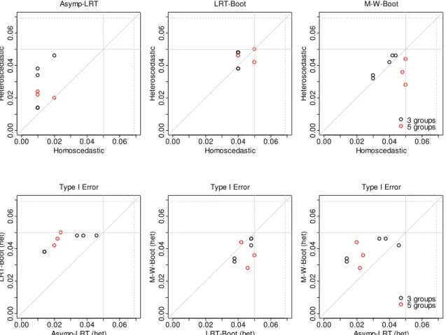
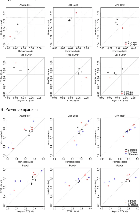
8. Type I Error and Power of homoscedastic tests on the normally distributed homoscedastic data... 58

9. Comparison of Type I Error and power of heteroscedastic tests on the normally distributed homoscedastic data... 59

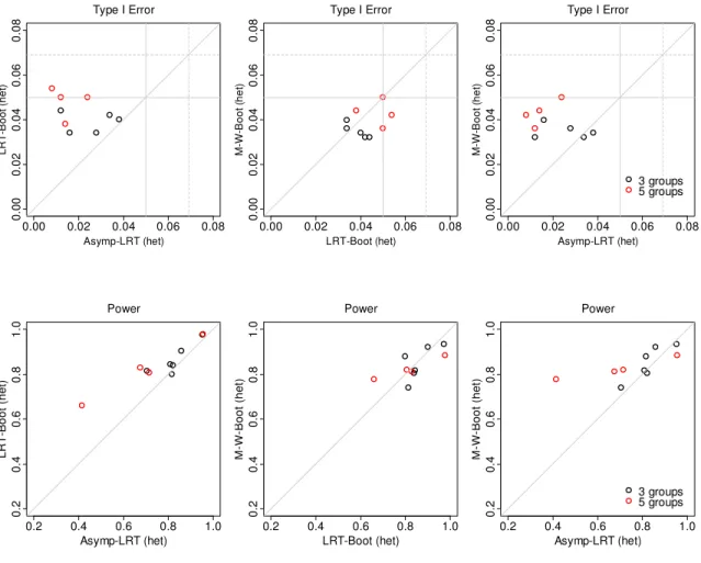
10. Type I Error and Power of heteroscedastic tests on the normally distributed heteroscedastic data ... 61

11. Comparison of Type I Error and Power of homoscedastic tests on the normally distributed heteroscedastic data... 62

12. Type I errors under the misspecified covariance matrix. ... 65

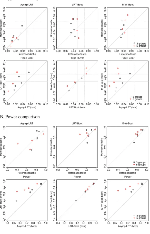
13. Type I Error and Power of homoscedastic tests on the log-normally distributed homoscedastic data... 67

14. Comparison of Type I Error and power of heteroscedastic tests on the log-normally distributed homoscedastic data ... 68

15. Type I Error and Power of heteroscedastic tests on the log-normally distributed heteroscedastic data ... 69

16. Comparison of Type I Error and Power of homoscedastic tests on the log-normally distributed heteroscedastic data ... 70

(12)

18. Type I errors of a proposed test for a mixture of two normally

distributed random variables ... 72 19. Type I errors of a proposed test when random errors follow the gamma distribution ... 73 20. Normal probability plots of organic mercury level in log-scale

for placebo and succimer groups. ... 77 21. Histograms of organic mercury level in log-scale for placebo and succimer groups... 77 22. Studentized residuals by time point... 78 23. Estimated mean blood log concentration of organic mercury in

(13)

CHAPTER 1 INTRODUCTION – LITERATURE REVIEW

1.1.Motivation

This dissertation work is motivated by problems encountered in the analysis of

some toxicological data and clinical trials data, where repeated measurements are made

on each subject, and the investigator expects trends in mean response among dose groups

and/or time points. For example, Cao et al., 2011 were interested whether succimer, a

mercaptan compound known to reduce blood lead concentration in children, also reduces

blood mercury concentration. They used samples from a randomized placebo-controlled,

double-blind trial clinical trial of succimer for lead poisoning in 780 children aged 12-33

months, called the Treatment of Lead-exposed Children trial, or TLC (Rogan, 1998). In

TLC, 384 children were assigned to the placebo group and 396 to the succimer group.

Up to three 26-day courses of succimer or placebo therapy were administered, depending

on response to treatment in those, who were given succimer. For children in each group,

blood lead concentrations were obtained twice before randomization and then on days 7,

28, and 42 after the beginning of each course of treatment. After treatment was stopped,

blood lead levels were measured every three to four months until 36 months after the

initiation of treatment. Cao et al. (2011) measured mercury in pre-treatment samples

(14)

in 1-week post-treatment blood samples (N = 768) and in a 20% random sample of the

338 children who received the maximum 3 courses of treatment.

In addition to the presence of variance components, the data can be potentially

heteroscedastic since the variability across time may not necessarily be constant. Very

little literature exists on constrained inference in linear mixed models even under

homoscedasticity, let alone under heteroscedasticity. Silvapulle (1997) proposed a

methodology for testing linear constraints regarding fixed effects parameters under some

conditions on the design matrices. The resulting test procedure does not depend upon the

unknown variance components, thus ignores correlations within the subject over time.

Thus the methodology developed in Silvapulle (1997) is restrictive and is not applicable

to the present context. As observed in Hoferkamp and Peddada (2002), the biggest

challenge in linear mixed models with or without heteroscedasticity is the derivation of

restricted maximum likelihood estimators (RMLE) for various parameters of the model.

Consequently, the derivation of the likelihood ratio test is non-trivial and has not been

derived in the literature so far.

Examples such as the above one are rather common in applications, and often

researchers tend to use the classical mixed effects analysis of variance followed by

“post-hoc” analyses to make pair-wise comparisons rather than testing for the desired order

restriction. There is clearly a demand for well developed theory and methodology for

such problems.

Another example that motivated this research is a recently published

(15)

dose of an investigational drug. The objectives of this trial were estimation of the mean

response (measured in minutes) under the assumption that mean responses are

constrained by an umbrella order and comparing the best dose with placebo and control.

Since each subject received two different doses (one of which was dose 0 mg, placebo),

unrestricted estimates of mean response were correlated. Instead of maximizing the

likelihood under restrictions while taking into account correlation structure, the

investigators obtained unrestricted estimates first, while taking into account correlation

structure and then obtained parameter estimates using a simpler method that is based on a

well known pool adjacent violators algorithm (PAVA) (Silvapulle and Sen, 2005). The

PAVA is used when non-decreasing order is assumed and proceeds as follows. If a pair

of adjacent unrestricted estimates violates the hypothesized order, then, according to the

algorithm, each such pair of estimates is replaced by their average. The process is

repeated until all estimates satisfy the hypothesized order. Although PAVA is a very

convenient methodology to implement, as described in the following sections, very little

is known about theoretical properties of PAVA.

Motivated by the above applications, in this dissertation research we will focus on

two aspects of constrained inference; (a) estimation of parameters for correlated data

subject to inequality constraints, and (b) testing hypothesis for correlated data under

inequality constraints. In section 1.2, we will review the literature on the estimation of

parameters under constraints, when the underlying data are correlated, and in section 1.3

(16)

1.2.Methods of estimation

Let

(

θ θ₁, ₂,..,θp

)

′ =

θ θθ

θ denote an unknown parameter vector whose components

satisfy inequality constraints. Problem of estimating parameters under constraints arises

for a variety of reasons. In some applications, such as in dose-finding clinical trials,

constrained estimation plays an important role for determining dose at which the next

patient needs to be treated (Stylianou and Flournoy, 2002; Ivanova et al., 2009; Conaway,

Dunbar and Peddada, 2004). In other situations, such as in toxicology, researchers are

often interested in testing for patterns of response. Again, in all such situations one needs

to perform constrained testing of parameters. For example, toxicologists are usually

interested in testing the hypothesis that the tumor incidence rate increases with the dose

of a toxin, i.e. testing H₀:θ₁=θ₂ =…=θ_p_against

1 2

:

A p

H θ ≤θ ≤…≤θ _{, known as}

simple order restriction (Peddada, Dinse and Kissling, 2007). Similarly, when

comparing multiple toxins with the control, toxicologists often test the hypothesis that the

tumor incidence due to a toxin is larger than the tumor incidence due to control, i.e., test

0: 1 2 p

H θ =θ =…=θ _against 1

:

A i

H θ ≤θ , i≥2, known as simple tree order. In all such situations, the test statistic requires the estimation of parameters under the inequalities

specified by the alternative hypothesis.

A variety of inequality constraints have been discussed in the literature, such as

the simple order θ₁≤θ₂ ≤…≤θ_p_{, the umbrella order}

1 2 i i 1 p

θ ≤θ ≤…≤θ ≥θ+ ≥…≥θ , the

single loop order, etc. (Stylianou and Flournoy, 2002; Ivanova et al., 2009; Conaway et

(17)

Often order restrictions can be expressed using graphs as shown in Figure 1. In

Chapter 3 we will focus on simple order restriction (a).

Figure 1. Examples of some order restrictions.

There exists over 50 years of literature on the estimation and testing of hypothesis

under inequality constraints on the parameters θ θ₁, ₂,..,θ_p in a variety of settings. For a

comprehensive review on estimation and testing of parameters under constraints, one

may refer to Silvapulle and Sen (2005) and van Eeden (2006). Much of the literature is

based on the likelihood principle. However, as reviewed in van Eeden (2006) and

Silvapulle and Sen (2005), several alternative estimation and testing procedures have

been proposed in the literature. They are often computationally simpler to implement and

are designed for the specific parametric model and specific order restrictions. Among

these methods, PAVA is one of the most popular methods for estimating parameters

under simple order restriction.

Suppose ˆUMLE

(

θˆ₁UMLE,θˆ₂UMLE,..,θˆUMLEp

)

′ =

θ θθ

θ is an unrestricted estimator of θθθθ , where

the components of ˆUMLE

(

ˆ₁UMLE, ˆ₂UMLE,.., ˆUMLE

)

p

θ θ θ ′

= θ θθ

θ are independently distributed, then

(18)

(

)

2 1

ˆ

min ,

p

UMLE

i i i

C i

w

θ

∈ =

−

∑

θ θθ

θ (1)

where C is the set of known inequalities satisfied by the components of θθθθ, and w_i is

some known weight, usually taken to be the reciprocal of the variance of

θ

ˆiUMLE.

If C is a subset of the parameter space satisfying simple order constraints, then the above minimization problem (1) is often solved by using the well-known pool

adjacent violator algorithm (PAVA) (cf. Silvapulle and Sen, 2005). Analytically, the

PAVA estimator for θ_i,i=1,2,...,p under θ₁≤θ₂ ≤...≤θ_p is given by the following equivalent formulae (cf van Eeden, 2006):

( )

1

ˆ

ˆ _{min max}

t

UMLE j j j s PAVA p

i _{i t p} _{s i} t j j s w

w

θ

=

≤ ≤ ≤ ≤

= =

∑

(2)

1

ˆ max min

t

UMLE j j j s

t i t p s i

j j s w

w

θ

=

≤ ≤ ≤ ≤

= =

∑

,

where

(

)

1 . ˆ

j _UMLE

j w

Var

θ

= The superscript (p) in _ˆPAVA p( )

i

θ denotes the PAVA estimate of

i

θ

based on p groups.

If the components of

θ

θθ

θ

ˆ

UMLE are independently and normally distributed with known variances, then PAVA results in the restricted maximum likelihood estimator

(19)

is derived by solving the following constrained minimization problem, where Σ is the (known) covariance matrix of

θ

θθ

θ

ˆ

UMLE:

(

)

1

(

)

C

ˆ ˆ

min UMLE − UMLE .

∈

′

− Σ −

θ θθ

θ

(3)

Diaz and González (1988) identified some sufficient conditions on Σ for which PAVA and RMLE are the same. For example, the sufficient conditions are satisfied

when _Σ is an intra-class correlation matrix. In general, however, they are not the same. If the unconstrained estimator is multivariate normally distributed, then the above

minimization problem results in RMLE. Again, we emphasize on the fact that PAVA, as

well as the solution to (3), provides robust estimators to θθθθ by not relying on the

knowledge of the underlying likelihood function which may not always be known.

Furthermore, the computation of the RMLE may not always be straightforward,

especially when _Σ is unknown (Shi, Zheng and Guo, 2005; Hoferkamp and Peddada, 2002). Also, as observed by several authors (cf. Lee, 1988; Fernandez, Rueda and

Salvador, 1999), the RMLE may not always perform well in terms of the mean squared

error even when Σ is known. Hwang and Peddada (1994) argued that the RMLE is not only universally dominated by the UMLE under certain conditions, but any fixed width

confidence interval centered at the RMLE may actually have a zero coverage probability

as p increases. They surprisingly note that the RMLE may fail even in the case of simple order when the underlying covariance matrix is non-diagonal.

As an example of the RMLE failing in the case of some specific covariance

matrix, let us discuss an example of star-shaped ordering presented by Shaked (1979).

Consider a species consisting of k individuals each of which has a quantitative

(20)

generation by

µ

_i+₁≥0. The expected value of X of the population in generation i is denoted by

θ

_i. Assume that k new individuals are produced in each generation, are added to the population, and that

µ

_i+₁≥

θ

_i (i.e. X is improving on the average). The

expected value of X in generation i is

(

1 2 ...

)

i i i

θ

=

µ

+

µ

+ +

µ

and

θ

i+₁≥

θ

i for all i=1,…,p−1. (4)

Figure 2. Star-shaped ordering

In this example _µ_µ_µ_µ=

(

µ µ₁, ₂,…,µ_p

)

_{satisfies star-shaped order restriction}

(

)

(

)

1 1 2 2 ... 1 2 ... p p

µ

≤

µ

+

µ

≤ ≤

µ

+

µ

+ +

µ

and θθθθ =

(

θ θ1, 2,…,θ_p

)

satisfies the

simple order restriction

θ

₁ ≤

θ

₂ ≤...≤

θ

_p. Thus, if X~ N( , )µµµµ I and

(

1

)

ˆ _... _,

i X Xi i

(21)

non-results indicate that RMLE is dominated by PAVA and, as the dimension p increases, it is also dominated by UMLE. These results are consistent with findings of Hwang and

Peddada (1994). This example is revisited on page 13.

PAVA is widely used even in situations where the unrestricted estimators are not

independently distributed, due to its computational simplicity. For instance, in clinical

trials involving repeated measurements on the same subject, Ivanova et al. (2009)

describe a proof-of-concept trial with crossover allocation, where PAVA was used to

estimate the target dose at the end of the trial. Other examples where PAVA was used for

correlated data include multidimensional scaling (Robertson, Wright and Dykstra, 1988),

non-parametric semi-variogram estimation (Kim and Boos, 2004), linear models with

covariates (Bretz, 2006), general constrained smoothing (Mammen, Marron, Turlach and

Wand, 2001), estimation of the baseline survivor function in a proportional hazard model

(Young, Jewell and Samuels, 2008; Li and Tseng, 2008), analysis of functional magnetic

resonance imaging (FMRI) data (Woolrich, Ripley, Brady and Smith, 2001), and ranking

and selection (Huang, 1984).

Shin et al. (1996) demonstrated that the solution to (3) is asymptotically equal to

the solution of

(

) (

1

)

C

ˆ ˆ

min UMLE UMLE

∈

′

− Ω −

θ θθ

θ θθθθ θθθθ θθθθ θθθθ , where

Ω

1 is a suitable diagonal matrix.

Thus by choosing suitable weights, one may solve the simpler isotonic regression

problem (1) using standard PAVA, which only requires a simple hand held calculator

rather than solving the optimization problem (3).

Although PAVA is widely used even when the components of

θ

θθ

θ

ˆ

UMLE are not independent, there do not seem to exist any results in the literature on the performance of

(22)

PAVA and solution to (3), with the exception of Diaz and González (1988) who identify

sufficient conditions under which PAVA provides the solution to (3).

In Chapter 2, PAVA will be evaluated in terms of mean squared error and

universal domination criterion (Hwang, 1985) under the assumption, that the unrestricted

estimator is multivariate normally distributed. For a pair of univariate estimators ηˆ₁ and

2

ˆ

η of a parameter

η

, ηˆ₁ is said to universally dominate (also known as stochastically

dominate) ηˆ₂ if for all η and all c>0, P

(

|ηˆ₁−η|<c

)

≥P

(

|ηˆ₂ −η|<c

)

with a strict inequality for some

η

. Equivalently, ηˆ₁ is said to universally dominate ηˆ₂ if

(

| ˆ1 |

)

(

| ˆ2 |

)

E_φ η −η _≤E_φ η −η _ for all non-decreasing functions

φ

with a strict inequality for some

η

. We demonstrate, that under certain conditions the RMLE

dominates the PAVA estimator in terms of the mean squared error when p=2, and that under certain conditions the PAVA estimator dominates the UMLE. In the case of p>2 we will consider a variety of covariance structures, that are commonly encountered in the

theory of experimental designs, clinical trials, econometrics, etc. Under certain

conditions on the elements of the covariance matrix we demonstrate that the PAVA

estimator universally dominates the UMLE. Since for certain patterns of covariance

matrices, the PAVA estimator and the RMLE are the same (Diaz and González, 1988),

thus, in such situations we actually derive universal domination results for the RMLE.

(23)

1.2.1. Some special covariance structures

Since it may not be possible to investigate the properties of the PAVA estimator

for arbitrary covariance matrices, in this dissertation the universal domination of the

PAVA estimator over the UMLE will be explored under some special covariance

structures. The covariance structures considered in this dissertation are described below.

1.2.1.1.Supplemented balance designs (SBD)

There exists an exhaustive amount of literature on experimental designs for

comparing treatment groups against a control group. For an efficient design it is well

known that the number of replicates for the control group should be larger than the total

number of treatment groups (Pearce, 1960). The basic idea of SBD is to “supplement”

(also referred to as “augment” or “reinforce”) a block design consisting of p−1 treatment groups by m replicates of the control group in each block. Typically these designs are such, that every pair of treatments occurs with equal frequency in all blocks,

and the frequency of co-occurrence of a treatment and the control is constant in all

blocks. Pearce (1960) termed these designs Supplemented Balance Designs (SBD). Properties of such designs have been well studied in the literature (Stufken, 1987;

Hedayat, Jacroux and Majumdar, 1988; Gupta, 1989). Consider a SBD where

observations are taken in blocks of size m+

(

p−1

)

n, with m observations in a block taken on the control treatment, i=1, and n observations taken on each of the treatments

2, ,

i= … p_{. Observations are normally distributed with variance}_σ2

. While

(24)

each block are assumed to be correlated with a correlation coefficient ρɶ_{. Denote}

[

]

2 2

1 1 (m 1) m

σ

=

σ

+ −

ρ

ɶ _, 2 2

[

]

2 1 (n 1) n

σ

=

σ

+ −

ρ

ɶ _and

[

1 (m 1)

]

m

[

1 (n 1)

]

n

ρ

=

+ − + −

ɶ

ɶ ɶ .

Let ˆθθθθUMLE denote the UMLE of θθθθ . The first component of θθθθ is the mean of the control group, and the remaining p−1 components are the means of the treatment groups. Then the variance-covariance matrix of the vector ˆ_θUMLE

θθ

θ is

2

1 1 2

2

1 2 2

σ

ρσ σ

σ

′

 

= 

 

Σ

K

1

1 , (5)

where 1 is a vector of 1s, ρ ≥ −1 (p−2) and K=(1−ρ)I+ρJ. As usual, I denotes the

(

p−1

) (

× p−1

)

identity matrix, and J is a

(

p−1

) (

× p−1

)

matrix of 1s (see Nigam et al., 1988, for more details).

Note that the above covariance structure also arises naturally in other contexts as

well, such as graphical models (Whittaker, 1990; Lauritzen, 1996), and lattice model

(Andersson and Perlman, 1993; Dempster, 1972). For a review on Σ one may refer to Sun and Sun (2005), where the authors consider a more general form of this matrix.

In this dissertation we focus on estimation of the control mean θ₁, the largest

mean θ_p and elementary contrasts of treatment means with the control mean θ_i−θ₁,

2, 3, ,

i= … p_{under the constraint that}

1 2 ... p

θ ≤θ ≤ ≤θ . In section 2.2 (page 23) we

present Theorem 2.2 demonstrating that in case of SBD covariance structure (5) and

(25)

the control and the highest dose groups. Supporting simulation results are presented in

Figure 5 and Figure 6.

We also argue that, since Theorem 2.2 also holds in the case of simple tree order

restriction as well, PAVA may perform better than UMLE for the control group in this

case. Results of supporting simulation studies are presented in Figure 7.

1.2.1.2.Designs where 1 is an eigenvector of the covariance matrix

There are many designs used in clinical trials and in other applications where

every principal sub-matrix of Σ has 1=(1,1,...,1) ' as an eigenvector. Some common examples include: (a) the intra-class covariance matrix of the form Σ=αI+βJ, where

J is a matrix of 1’s, (b) cross-over designs where patients in Group A receive treatments

1, 3, 5, etc, patients in Group B receive treatments 2, 4, 6, etc; all observations have the

same variance, and the correlation coefficient within subject is same in both groups, and

(c) covariance matrix of elementary contrasts

(

2 1 3 1 1

)

ˆ ˆUMLE ˆUMLE_, ˆUMLE ˆUMLE_,..., ˆUMLE ˆUMLE p

θ θ θ θ θ θ ′

= − − −

δδδδ in a SBD.

1.2.1.3.Covariance matrix in a star-shaped ordering

Suppose X ~ N( , )

µ

I , then the components of

µ

are said to satisfy a star-shaped order if µ₁≤

(

µ₁+µ₂

)

2≤...≤

(

µ₁+µ₂ +...+µ_p

)

p. As discussed in Shaked (1979) and Dykstra and Robertson (1982), star-shaped order restriction arises naturally in many

applications. Performing a liner transformation θˆ_i =

(

X₁+...+ X_i

)

i, we have ˆ ~ ( , )N Σ

θ θ

θ θ with

θ

_i =

(

µ

₁+...+

µ

_i

)

i satisfying the simple order restriction p

θ

(26)

1 1 2 1 3 1

1 2 1 2 1 3 1

1 3 1 3 1 3 1

1 1 1 1

p p p

p p p p

 

 

=

 

 

Σ

… … …

⋮ ⋮ ⋮ ⋱ ⋮

…

. (6)

In section 2.2 (page 29), we present Theorem 2.3 demonstrating that in case of

star-shaped order restriction on the mean components, PAVA may perform better than

UMLE for the control group. Supporting simulation results are presented in Figure 3.

1.3.Testing of hypotheses

Testing hypotheses under inequality constraints is a well researched area. For a

comprehensive account, one may refer to the recent book by Silvapulle and Sen (2005).

In addition to the standard likelihood ratio test, a variety of alternative tests are available

for comparing means of two or more independent normal populations when no covariates

are present. Suppose θθθθˆUMLE ~N( ,θθθθ σ2I) and suppose one is interested in testing the following hypotheses regarding the components of θθθθ , where the alternative hypothesis is

the simple tree order

0: 1 2 p versus A: 1 i, 2

H θ =θ =…=θ H θ ≤θ ≤ ≤i p

(with at least one strict inequality). In addition to the classical likelihood ratio test, a

popular alternative test for testing the above hypotheses is the Dunnett’s test (Dunnett,

1955), which is defined as follows. For an elementary contrast θ_i −θ₁, the UMLE is

1

ˆUMLE ˆUMLE i

θ

−

θ

, i≥2. An estimator of the variance of this estimator is given by

(

_ˆ _ˆ

)

2

ˆ UMLE UMLE ₂_ˆ

(27)

linear model. The Dunnett’s test statistic is given by max ˆ_iUMLE ˆ₁UMLE ˆ 2 .

i θ −θ σ As

noted by Marcus and Talpaz (1992), a potential weakness of this statistic is that its

numerator does not use the inequality constraint specified by the alternative hypothesis.

Accordingly, they modified the numerator of the statistic by replacing the UMLE by the

RMLE of θθθθ under the simple tree order constraint. Although the resulting test improves

the power of Dunnett’s test for certain choices of θθθθ , it is surprising that it does not

improve the power uniformly for all θθθθ . More recently Tang and Lin (1997) introduced

an Approximate Likelihood Ratio (ALR) test that can be used for testing the above

hypothesis. A distinct advantage of ALR is that it is computationally simple to

implement for any p and it performs very well in terms of power in comparison to both the classical likelihood ratio test as well as Dunnett’s test for certain choices of θθθθ . The

procedure of Marcus and Talpaz (1992) was inspired by the earlier papers of Williams

(1971, 1972, 1977). In his 1971 and 1972 papers, Williams discussed the problem of

comparing means of the treatment groups with the control group in a dose response study

where the population means are assumed to be non-decreasing with dose (i.e.

1 2 ... p

θ ≤θ ≤ ≤θ ). In Williams (1971) the test statistic was

(

1

)

ˆ ˆ

ˆ 2

RMLE UMLE p

θ

σ

−

, where as in

Williams (1972) he used

(

1

)

ˆ ˆ

ˆ 2

RMLE RMLE p

θ

σ

−

, where

θ

ˆRMLE is the RMLE under the simple

order constraint. In his 1977 paper, Williams considered the problem of testing

0: 1 2 ... p

H

θ

=

θ

= =

θ

versus Ha:

θ

1≤

θ

2 ≤...≤

θ

p (with at least one strict inequality)

using the statistic

(

1

)

ˆ ˆ

ˆ 2

RMLE RMLE p

θ

σ

−

(28)

Nonparametric versions of Dunnett's test and Williams’ test were also developed

in the literature using rank based methods by Dunn (1964) and Shirley (1977),

respectively. These methods are widely used in practice for their practical simplicity, and

simulation studies reported in the literature suggest, that these methods compete very

well against the likelihood ratio tests.

It is reasonable to anticipate or assume a monotonic mean response in dose

response studies conducted by toxicologists. In such situations, the Williams’ test (1972,

1977) tends to have a higher power than the Dunnett’s test when comparing the mean

response at the highest dose with that of the control group. However, there are instances

where, perhaps due to toxicity at high doses, the mean response at the higher doses may

change direction resulting in a down-turn (or up-turn) in the mean response. In such

situations, the Williams’ test (1972, 1977) loses power in comparison to the Dunnett’s

test when comparing the mean of the highest dose with the control. Typically, in the

analysis of their 90 day pre-chronic rodent cancer studies, the National Toxicology

Program (NTP) uses either Dunnett’s test or Williams’ test depending upon the data –

which is unsatisfactory. Since in practice it is not feasible to determine a priori whether

the departure from monotonic response will take place or not, it is important to develop a

method that would be robust to both possibilities. In Peddada et al. (2006) such a robust

procedure was developed using the point estimators developed in Hwang and Peddada

(1994). The resulting methodology seems to perform as well as the Williams’ test when

the mean responses are monotonic in dose and performs as well as Dunnett’s test when

(29)

In many applications such as in epidemiology, researchers are often interested in

testing for the equality of mean responses of various groups against the alternative

hypothesis that the means are constrained by some inequality constraints, after adjusting

for various covariates. Often such problems can be formulated using fixed effects linear

models and applying the likelihood ratio methodology as detailed in Silvapulle and Sen

(2005). Several variations to the likelihood ratio principle have been proposed in the

literature. As previously stated, the likelihood ratio principle provides a rich framework

to conduct the analyses of such data. In the presence of covariates (whether continuous

or categorical), the unrestricted estimators of treatment means are not necessarily

independently distributed. In such a case, as noted in the previous sections and in Hwang

and Peddada (1994) and others, the RMLE may not perform well as an estimator of the

mean vector. Consequently, one cannot assume that the likelihood ratio based methods

would perform well in terms of power since they use RMLE. For this reason, Betcher

and Peddada (2009) developed a Dunnett-type test statistic that uses a modified RMLE as

the point estimator of the mean vector. Based on the simulation studies reported in

Betcher and Peddada (2009), in the case of simple order, their new method provides

better confidence intervals than those based on RMLE.

Constrained inference in linear mixed effects models arises naturally in many

applications, such as the ones described in this Chapter1. Specifically, they arise

naturally in the context of repeated measurement designs. Silvapulle (1997) proposed a

simple methodology for testing linear constraints regarding fixed effects parameters

under some conditions on the design matrices. The resulting test procedure does not

(30)

In the case of general mixed effects models, a natural strategy for testing for

inequalities among treatment effects after adjusting for covariates would be to develop a

likelihood ratio test. Such a strategy necessarily requires the derivation of RMLE under

inequality constraints. As noted in the literature, this is a very challenging problem.

Hoferkamp and Peddada (2002) proposed an EM based algorithm for estimating

regression parameters under constraints, when the error variances are heteroscedastic and

potentially subject to inequality constraints. Under some conditions on design matrices,

they discussed the convergence of their algorithm. Recently, Shi et al. (2005) addressed

the problem in a slightly different context. They considered the usual fixed effects model

but allowed the error variance to be multivariate normally distributed with an unknown

non-diagonal covariance matrix Σ. Thus, unlike the linear mixed effects model where

Σ has a special structure, in Shi et al. (2005) it was not constrained by a particular structure.

They developed EM algorithm to estimate regression parameters subject to

inequality constraints in such a linear model and identified conditions under which the

EM algorithm converges. None of these papers discusses the problem of testing

regression parameters under constraints in a linear mixed effects model. They are all

limited to the constrained estimation problem and none of these papers address the testing

problem.

Apart from the earlier attempts in some special cases, tests for linear mixed

models under inequality constraints on the fixed effects parameters has not been well

(31)

case when normal populations are correlated as in a repeated measurements design. In

this paper, the author does not include any covariates. Silvapulle (1997) generalized

Mukerjee (1988) to some unbalanced designs with incomplete data. He noted that

within-subject correlations make it difficult to generalize some tests into repeated models.

Earlier, Singh and Wright (1990) considered order restricted inference on fixed effects in

a two-factor mixed model. They presented an analogue to the usual F-test for homogeneity and obtained several closed-form results.

There did not exist a systematic general methodology for the analysis of linear

mixed effects models, when the regression parameters are subject to inequality

constraints, until Davidov and Rosen (2011), who derived the likelihood ratio test for

testing the hypotheses of the type H₀:

η

=0 vs H_A:

η

≥0 when 2

N

σ =

Σ I . In Section 3.2, the likelihood ratio test of Davidov and Rosen (2011) is reviewed, and in Section 3.3,

the likelihood ratio test under heteroscedastic error structure

1 2

2 2 2

1 n : 2 n : : k nk

diag

σ



= _ _

Σ I I … I _{is derived. Motivated by various limitations of these}

likelihood ratio tests, in Section 3.4 an EBLUP bootstrap methodology is described under

homoscedastic as well as heteroscedastic error structures. An alternative method

analogous to Williams (1971) and based on Rao’s MINQUE theory (1970, 1971, 1972) is

explored in Section 3.5. In Chapter 4, extensive simulation studies are performed to

evaluate the performance of various tests in terms of the Type I error and power. Since

very limited literature is available for this very important practical problem, this

dissertation work extends the existing knowledge in this field substantially. The

proposed methodologies are illustrated in Chapter 5 using the recently published

(32)

CHAPTER 2 CONSTRAINED ESTIMATION AND THE PERFORMANCE

OF PAVA

In this section, we will describe some of the theoretical and simulation results

obtained so far in this dissertation with regards to the constrained estimation problem.

Proofs of theorems are presented in Appendix A.

We assume that UMLE of θθθθ ,

θ

θθ

θ

ˆUMLE, is distributed according to a multivariate normal distribution with mean θθθθ and covariance matrix Σ. As often done, without loss of generality, unless stated otherwise, we assume the sample size of 1, because it can be

absorbed in _Σ. In general, the order restricted estimators (whether RMLE or other constrained estimators) do not always perform well in all settings. Their performance

depends upon the type of inequality constraints as well as the covariance structure and the

dimension p (cf. Lee, 1988; Hwang and Peddada, 1994; Fernandez et al., 1999).

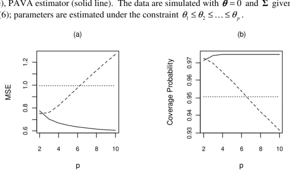
To illustrate this point, we provide results of a small simulation study in Figure 3.

In this study, we simulated data from a -variatep normal distribution with mean vector 0

= θ θθ

θ and covariance matrix Σ given by (6).

Under the constraint

θ

₁ ≤

θ

₂ ≤…≤

θ

_p_{, we estimated the MSE of the UMLE,}

(33)

PAVA estimator, i.e. P

(

θ

ˆ₁UMLE−

θ

₁ <1.96

)

, P

(

θ

ˆ₁RMLE −

θ

₁ <1.96

)

and

(

ˆ1 1 1.96

)

PAVA

P

θ

−

θ

< (Figure 3 (b)). We chose the value of 1.96, because for this value

of the critical constant, the confidence interval centered at UMLE has a coverage

probability of 0.95. All results are based on 100,000 simulation runs.

Figure 3. MSE and Coverage Probability of

θ

₁: UMLE (dotted line), RMLE (dashed line), PAVA estimator (solid line). The data are simulated with θθθθ =0 and Σ given by (6); parameters are estimated under the constraint

θ

₁≤

θ

₂ ≤…≤

θ

_p_.

From the Figure 3, it is clear that for the covariance matrix considered in this

example, the RMLE performs poorly both in terms of MSE as well as the coverage

probability, as p increases, while the PAVA estimator performs the best. In view of the above illustration and the fact that PAVA is widely used in practice even for correlated

data, we investigate its performance relative to UMLE in terms of universal domination

criterion.

2 4 6 8 10

0

.6

0

.8

1

.0

1

.2

(a)

p

M

S

E

2 4 6 8 10

0

.9

3

0

.9

4

0

.9

5

0

.9

6

0

.9

7

(b)

p

C

o

v

e

ra

g

e

P

ro

b

a

b

ili

(34)

2.1.Performance of PAVA in the case of p = 2

We begin by comparing the MSE of the UMLE, RMLE and PAVA estimator for

2

p= to demonstrate that, even in this simple setting, the performance of PAVA can depend upon the underlying correlation structure. We assume that ˆUMLE

(

,

)

N Σ

∼

θ θ

θθ θθ

θ θ ,

1 2

θ

≤

θ

and the elements of Σ have no special structure with Var

(

θ

ˆ₁UMLE

)

=

σ

₁2,

(

)

2

2 2

ˆUMLE

Var

θ

=

σ

, and Cov

(

θ

ˆ₁UMLE,

θ

ˆ₂UMLE

)

=

ρσ σ

₁ ₂.

Theorem 2.1:

(a) If

ρ

≤0 and either

θ

₂ ≥

θ

₁≥0 or 0≥

θ

₂ ≥

θ

₁, then

E(

θ

ˆ₂PAVA −

θ

₂)2 ≤E(

θ

ˆ₂ −

θ

₂)2;

(b) if

θ

₁≤

θ

₂ and

ρ σ

( ₂ −

σ

₁)(

ρσ

₂ −

σ

₁)≥0, then

E(

θ

ˆ₂RMLE −

θ

₂)2≤E(

θ

ˆ₂PAVA−

θ

₂)2.

To understand the performance of PAVA in the case, when the sufficient

conditions of Theorem 2.1 are not true, we simulated the data from bivariate normal

distributions with mean vector

(

0, 0

)

′,

σ

₁ =1,

ρ

=0.9 and

σ

₂ ranging from 0.1 to 1.4.

Under the constraint θ₁≤θ₂, the estimated MSE of UMLE, RMLE and PAVA estimator

(35)

Figure4. MSE of

θ

₂ as a function of

σ

₂: UMLE (dotted line), RMLE (dashed line), PAVA estimator (solid line). The data are simulated with

θ

₁ =

θ

₂ =0,

ρ

=0.9,

σ

₁=1; parameters are estimated under the constraint

θ

₁≤

θ

₂. Shaded area shows the values of

2

σ

, where the conditions of Theorem 2.1 are satisfied, i.e.,

σ

₂ ≥

σ ρ

₁ .

0.2 0.6 1.0 1.4

0

.0

0

.5

1

.0

1

.5

2

.0

σ₂

M

S

E

Theorem 2.1, together with Figure4, suggests that the performance of PAVA

depends upon the underlying correlation structure even in the case of p=2. We note from Figure4, that RMLE performs better than PAVA for the choice of parameters

considered in this simulation study. In view of the above findings, we deduce that

domination results may not exist for arbitrary covariance structures when p>2. Therefore in section 2.2 we consider some covariance structures that arise naturally in

many applications and investigate the performance of PAVA relative to UMLE for those

structures.

2.2.Performance of PAVA for p > 2 under various covariance structures

2.2.1. SBD covariance structure

It is well-known that in many situations the total MSE of the RMLE is smaller

than that of the UMLE (cf. Fernandez et al., 1999). Surprisingly, based on a small

(36)

estimator is not only smaller than the total MSE of the UMLE but it is almost as small as

the total MSE of the RMLE, if not smaller. We find this to be an interesting and a

surprising result. In this simulation experiment,

θ

θθ

θ

ˆUMLE, the UMLE of

θθ

θ

, was generated according to a multivariate normal distribution with mean

θθ

θ

and the covariance matrix given by (5), p=10,

σ

₁=1 and

ρ

=0.4. However, since it is well-known that

reduction in the total MSE does not necessarily imply a reduction in the MSE of

individual coordinates (Lee, 1988; Fernandez et al., 1999), in Figure 6 we investigated

the performance of the PAVA estimator of the control mean

θ

₁ and the largest mean

θ

_p

in terms of universal domination criterion. We identify sufficient conditions, under which

PAVA performs better than UMLE. Recall from Hwang (1985) that universal

domination is equivalent to domination in terms of all monotonic functions of quadratic

loss and hence implies domination in terms of MSE. Analytical comparisons between

PAVA and RMLE appear to be intractable and hence are not discussed here.

Theorem 2.2: Suppose _θ_θ_θ_θˆUMLE ∼N

(

_θ_θ_θ_θ,_Σ

)

_{, where}_Σ_{is of the form (5) and suppose}

1 2 ... p

θ ≤θ ≤ ≤θ .

(a) If either

2 2

1 2

( 1 / )

0,

( 1)( 2 2 / )

p

p p

σ

ρ

σ

− +

− < <

− − +

σ

1 <

σ

2 or

ρ

>0,

σ

1 >

σ

2, then for

all c>0, P

(

θ

ˆ₁PAVA p( ) −

θ

₁ <c

) (

≥P

θ

ˆ₁UMLE−

θ

₁ <c

)

.

(b) If either

2 2

1 2

( 1 / )

0,

( 1)( 2 2 / )

p

p p

σ

ρ

σ

− +

− < < >

− − + or

1 2

0

ρ

σ

1

σ

< < < , then for all

c>0,

(

_ˆPAVA p( )

) (

_ˆUMLE

)

p p p p

(37)

Figure 5. Total MSE as a function of

σ

₂: UMLE (dotted line), RMLE (dashed line), PAVA estimator (solid line). The data are simulated with p=10,

θ

_i =0, i=1,…, ,p _Σ

given by (5),

ρ

=0.4,

σ

₁=1; parameters are estimated under the constraint

1 2 p

θ

≤

θ

≤…≤

θ

_.

0 2 4 6 8 10

0

2

0

6

0

σ₂

T

o

ta

l

M

S

E

We performed extensive simulation studies to compare UMLE, RMLE and

PAVA including the situations where the sufficient conditions of the above theorem are

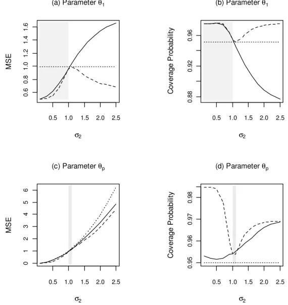
not satisfied. A small sample of the results is provided in Figure 6. As expected, PAVA

performs well in terms of MSE as well as the coverage probability, when the sufficient

conditions of Theorem 2.2 are satisfied. However, its performance can be rather poor

when the sufficient conditions are not satisfied. It is important to recognize that the

sufficient conditions provided in parts (a) and (b) of Theorem 2.2 are disjoint. Together

with the fact that simulation results suggest these conditions may even be necessary, we

(38)

Figure 6. MSE and Coverage Probability of

θ

₁ and

θ

p as a function of

σ

2: UMLE

(dotted line), RMLE (dashed line), PAVA estimator (solid line). The data are simulated with p=5,

θ

_i =0, i=1,…,p_,_Σ_{given by (5),}

_ρ

₌_0.9_,

1 1

σ

= ; parameters are estimated under the constraint

θ

₁≤

θ

₂ ≤…≤

θ

_p_{. Shaded area shows the values of}

2

σ

, where the conditions of Theorem 2.2 are satisfied, i.e.

σ

₂ <

σ

₁ for (a), (b) and

1 2 1

σ

<

σ

<

σ ρ

for (c), (d).

0.5 1.0 1.5 2.0 2.5

0

.6

0

.8

1

.0

1

.2

1

.4

1

.6

(a) Parameter θ₁

σ2

M

S

E

0.5 1.0 1.5 2.0 2.5

0

.8

8

0

.9

2

0

.9

6

(b) Parameter θ₁

σ2

C

o

v

e

ra

g

e

P

ro

b

a

b

ili

ty

0.5 1.0 1.5 2.0 2.5

0

1

2

3

4

5

6

(c) Parameter θ_p

σ₂

M

S

E

0.5 1.0 1.5 2.0 2.5

(d) Parameter θ_p

σ₂

C

o

v

e

ra

g

e

P

ro

b

a

b

ili

ty

0

.9

5

0

.9

6

0

.9

7

0

.9

8

Note that the proof of Theorem 2.2 does not use any information regarding the

(39)

1 ( ) 1 1 1 ˆ

ˆ _min _.

t UMLE j j j PAVA p t t p j j w w θ θ = ≤ ≤ = =

∑

Corollary 1: Suppose _θ_θ_θ_θˆUMLE ∼ N

(

_θ_θ_θ_θ,Σ

)

_{, where}_Σ_{is of the form (5) and suppose}

1 i

θ ≤θ ,

2

i ≥ . If either

2 2

1 2

( 1 / )

0,

( 1)( 2 2 / )

p p p σ σ ρ σ σ − +

− < <

− − + σ1 <σ2 or ρ >0, σ1 >σ2, then

for all c>0, P

(

θ

₁ <c

) (

≥P

θ

ˆ₁UMLE −

θ

₁ <c

)

.

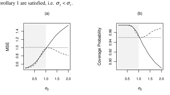
Again, as above, the simulation results provided in Figure 7 suggest that PAVA

performs very well relative to both UMLE and RMLE when the sufficient conditions of

Corollary 1 are satisfied (shaded area). Otherwise, its performance can be very poor

(unshaded area).

Figure 7. MSE and Coverage Probability of θ₁ as a function of σ₂: UMLE (dotted line), RMLE (dashed line), PAVA estimator (solid line). The data are simulated with p=5,

0

i

θ

= , i=1,…,p_,_Σ_{given by (5),}

_ρ

₌_0.9_,

1 1

σ

= ; parameters are estimated under the constraint θ₁ ≤θ_i, i ≥2. Shaded area shows the values of σ₂ where the conditions of Corollary 1 are satisfied, i.e. σ₂ <σ₁.

0.5 1.0 1.5 2.0

0 .6 0 .8 1 .0 1 .2 1 .4 (a) σ₂ M S E

0.5 1.0 1.5 2.0

(40)

2.2.2. Covariance matrices where 1 is an eigenvector

Recall the design described in section 1.2 on page 13, where every principal

sub-matrix of Σ has 1=(1,1,...,1) ' as an eigenvector. Following arguments similar to those

in the proof of Theorem 2.2 or by appealing to Hwang and Peddada (1994), we deduce

the following important corollary. Note that, different from Theorem 2.2, the following

result applies to all coordinates of the mean vector .θθθθ

Corollary 2: Suppose _θ_θ_θ_θˆUMLE ∼N

(

_θ_θ_θ_θ,_Σ

)

_._{If every principal sub-matrix of}_Σ_has

(1,1,...,1) '

1= as an eigenvector, and suppose that

θ

₁ ≤

θ

₂ ≤...≤

θ

_p, then for all 1, 2,...,

i= p and c>0, P

(

θ

ˆ_iPAVA p( )−

θ

_i <c

) (

≥P

θ

ˆ_iUMLE −

θ

_i <c

)

.

In the case of intra-class covariance structure, from Theorem 2.2 of Diaz and

González (1988), we deduce that RMLE and PAVA are identical. Hence in that case the

above corollary applies to RMLE as well.

2.2.3. Star-shaped order covariance structure

Recall the star-shaped order restriction (defined in section 1.2.1 on page 13) with

covariance matrix _Σ given by (6). Appealing to Theorem 2.2 in Diaz and González (1988) we note that PAVA and RMLE of µ are the same, but PAVA and RMLE of θ

are not the same. As observed in the simulation study reported in Figure 3, RMLE of θ₁

(41)

Theorem 2.3: Suppose _θ_θ_θ_θˆUMLE ∼ N

(

_θ_θ_θ_θ,Σ

)

_{, where}

(

)

1, 2,..., p

θ θ

θ

=

θ

θθ

θ

,

θ

₁≤

θ

₂ ≤...≤

θ

_p, and Σ is given by (6). For all c>0, P

(

θ

₁ <c

) (

≥P

θ

ˆ₁UMLE −

θ

₁ <c

)

.

2.3.Conclusions and recommendations

Often in clinical trials repeated measurements are made on each subject, the

investigator expects trends in the mean response among dose groups and/or time points,

and the problem of interest is to estimate and test parameters under such constraints on

the mean responses. For example, Ivanova et al. (2009) describe such a Phase II trial,

where each patient received control and two doses of the drug. The Pool Adjacent

Violators Algorithm (PAVA) was designed for estimating parameters under the simple

order restriction (i.e. increasing or decreasing order among the mean responses), when

unrestricted estimators of parameters are independent. However, PAVA is also often

used even when unrestricted estimators are correlated. Based on the results obtained in

this research, it appears that simple PAVA based algorithms may be reasonable even if

the unrestricted estimators are correlated.

For example, in a Supplemented Balance Design (SBD), where a researcher is

interested in estimating elementary contrasts of each dose group with the control group

(under the constraint that the mean responses are monotonic in dose), we found that the

confidence interval centered at PAVA estimate of an elementary contrast between the

dose group and the control group will have larger coverage probability than the

confidence interval centered at the UMLE of the contrast. Thus, PAVA is recommended

over UMLE for estimating all elementary contrasts of dose groups with the control group.

(42)

covariance matrix of the sample mean vector has an intra-class covariance structure and

satisfies the conditions of Corollary 2; thus, PAVA is recommended over UMLE for

estimating all treatment means under the simple order constraint, and also, all elementary

contrasts when they are subject to the simple order constraint. We also note that for

estimating the control group mean (under either simple order or simple tree order

restriction on treatment means), the PAVA performs better than the UMLE if: 1) the

variance in the control group is smaller than the variance in the treatment group and the

correlation between groups is negative or 2) the variance in the control group is larger

than the variance in the treatment group, and the correlation between groups is positive.

There are situations in clinical trials, when a large number of treatments need to

be compared, and not all treatments can be present in each block. In such case, a

balanced incomplete block design (BIBD) may be considered. For illustration, consider a

dose-response study consisting of control, low-dose and high-dose groups of a drug, and

litters of mice are taken to be blocks. A BIBD can be constructed as follows. Suppose

each block (litter) consists of two pups. The pups in the first block are randomly

assigned to either control or low-dose group; pups in the second block are randomly

assigned to either control or high-dose group; and the pups in the third block are

randomly assigned to the low or high-dose group. The resulting design is a BIBD.

A feature of a BIBD is that all blocks have the same number of treatments, and all

treatments, as well as all pairs of treatments, are observed the same number of times in

the experiment. Furthermore, the correlation coefficient between sample means is

(43)

BIBD has an intra-class covariance structure. Thus, the covariance matrix satisfies the

conditions of Corollary 2. Note that the randomized complete block design (RCBD) can

be thought as a special case of BIBD. Thus, Corollary 2 also applies to an RCBD. Thus,

in these cases PAVA is recommended over UMLE for estimating all treatment means

under the simple order constraint, and more importantly, all elementary contrasts when

they are subject to simple order constraint. Again, a confidence interval centered at

PAVA of any such contrast will have larger coverage probability than the confidence

interval centered at the UMLE of the contrast.

Analytical comparisons between PAVA and RMLE appeared to be intractable and

hence were not discussed in Chapter 2. However, performed simulations indicate that the

RMLE might perform better or worse than PAVA, depending on the covariance matrix of

the UMLE. It is known that in many situations the total mean squared error (MSE) of the

RMLE is smaller than that of the UMLE. Surprisingly, based on a small simulation study

under SBD, when the variance in the control group is smaller than the variance in the

treatment group, and the correlation between groups is positive, we discover that the total

MSE of the PAVA estimator is not only smaller than the total MSE of the UMLE, but it

is also smaller than the total MSE of the RMLE. Note, that if variances of the control

group and treatment group under a SBD are equal, RMLE and PAVA estimates of

treatment means under the simple order constraint are the same. Star-shaped order is a

known example where the RMLE does not perform well. We have shown that PAVA is

superior to UMLE as well as RMLE for estimating the control mean in the case, where

(44)

In general, it may not be possible to recommend an estimation procedure for an

(45)

CHAPTER 3 CONSTRAINED TESTING IN A LINEAR MIXED EFFECTS

MODEL

Motivated by the data of Cao et al. (2011) discussed in Chapter 1, the focus of this

chapter is to develop statistical methodology for performing constrained inference on the

location parameters of a linear mixed effects model, where covariance structure is of the

form Cov( )Y =UTU′+_Σ, where T and _Σ are diagonal matrices. Although such a structure is reasonable in the motivating example and is often used when analyzing

repeated measures data (cf. Khattree and Naik, 1999), in general, however, depending

upon the application, the covariance structures may be more complicated or unspecified.

For example, in a random slopes model for repeated measurement designs, it is common

to have the structure of T to be of the form T= ⊗I Ω, where Ω is a non-diagonal matrix. A common choice for _Ω is the auto-correlation structure. There are also

instances where the structure of the covariance matrix Cov( )Y may not be pre-specified. In Sections 3.2 and 3.3 we describe the likelihood ratio tests (LRT), developed in

Davidov and Rosen (2011) for constrained inference in linear models with covariance

Estimation and testing of parameters under constraints for correlated data