Integration of spatio-temporal vegetation dynamics into a distributed ecohydrological model : application to optimality theory and real-time watershed simulations

INTEGRATION OF SPATIO-TEMPORAL VEGETATION DYNAMICS INTO A

DISTRIBUTED ECOHYDROLOGICAL MODEL: APPLICATION TO

OPTIMALITY THEORY AND REAL-TIME WATERSHED SIMULATIONS

Taehee Hwang

A dissertation submitted to the faculty of the University of North Carolina at Chapel Hill

in partial fulfillment of the requirements for the degree of Doctor of Philosophy in the

Department of Geography

Chapel Hill

2010

Approved by:

Lawrence E. Band, Advisor

Aaron Moody, Reader

Conghe Song, Reader

Gregory W. Characklis, Reader

iii

ABSTRACT

Taehee Hwang

Integration of spatio-temporal vegetation dynamics into a distributed ecohydrological model: Application to optimality theory and real-time watershed simulations

(Under the direction of Lawrence E. Band)

iv

flowpaths leads to system-wide emergent optimality for carbon uptake over and above the individual patch. Lateral hydrological connectivity determines the degree of dependency on productivity and resource use with other patches along flowpaths, resulting in different system-wide carbon and water uptake by vegetation. In Chapter 3, phenological signals are extracted from global satellite products to find the topography-mediated controls on vegetation phenology in the study site. It provides a basis to understand spatial variations of local vegetation phenology as a function of microclimate, vegetation community types, and hillslope positions. In Chapter 4, near real-time vegetation dynamics are estimated by fusing multi-temporal satellite images, and integrated into the catchment scale distributed ecohydrological simulation. Integration of spatio-temporal vegetation dynamics into a distributed ecohydrological model helps to simulate

v

DEDICATION

This dissertation is dedicated

vi

ACKNOWLEDGEMENTS

First, I would like to thank my advisor, Dr Lawrence Band who deepened and broadened my scope of research views. Considering broad topics of my dissertation, I was so lucky to meet such an open-minded advisor with consistent enthusiasm and a positive manner. He is my role model not only for an academic advisor but also as a lifetime mentor.

I am also grateful to other committee members, Dr. Aaron Moody, Dr. Conghe Song, Dr. Greg Characklis, and Dr. Jim Clark. I learned a lot from their classes over the years. Even though I did not finish all I suggested, they encouraged me and showed interests to my researches from different perspectives. In addition, I would like to thank Dr. Jim Vose, Dr. Paul Bolstad, and Dr. Todd Lookingbill for their support in providing data in Coweeta Hydrologic Lab. I also like to thank my colleagues and friends who worked with me in the fields and helped me for the completion of this dissertation. During pit-digging experiments in the fields, Dr. T.C. Hales broadened my geological views also with impressive untiring energy. Tamara Mittman and Jon Duncan also gave valuable feedbacks to improve my dissertation both academically and grammatically.

vii

TABLE OF CONTENTS

LIST OF TABLES ... xii

LIST OF FIGURES ... xiii

LIST OF ABBREVIATIONS ... xix

LIST OF SYMBOLS ... xxi

Chapter 1

Introduction ... 1

1.1

Background ... 1

1.2

A Process-based Distributed Ecohydrological Model ... 4

References ... 8

Chapter 2

Ecosystem processes at the watershed scale: Extending optimality

theory from plot to catchment ... 12

2.1

Abstract ... 12

2.2

Introduction ... 13

2.3

Model overview... 16

2.3.1

A Farquhar photosynthesis model ... 16

2.3.2

Coupled photosynthesis – stomatal conductance models ... 18

viii

2.3.4

Nitrogen limitation ... 20

2.3.5

Allocation ... 21

2.4

Materials and methods ... 24

2.4.1

Site description... 24

2.4.2

Climate data and historical field measurements ... 26

2.4.3

Hydrologic gradients of vegetation density ... 27

2.4.4

Rooting depth and root distributions from soil pits ... 30

2.4.5

Model parameterization ... 33

2.4.6

Prescribed rooting depth as a function of hillslope position ... 36

2.4.7

Allocation dynamics with varying rooting depth... 40

2.5

Results ... 41

2.5.1

Topographic controls on rooting depth ... 41

2.5.2

Parameter spaces ... 43

2.5.3

Long-term ecohydrologic optimality at the hillslope scales ... 45

2.6

Discussion and conclusions ... 49

2.6.1

Optimal vegetation gradients for system-wide productivity ... 49

2.6.2

Compromises between multiple resources... 50

2.6.3

An objective function of optimality models ... 53

2.6.4

Allocation dynamics along the hillslope gradients ... 54

2.6.5

Limitations of this study ... 56

ix

Acknowledgements ... 58

References ... 59

Chapter 3

Topography-mediated controls on local vegetation phenology estimated

from MODIS vegetation index ... 71

3.1

Abstract ... 71

3.2

Introduction ... 72

3.3

Materials and methods ... 74

3.3.1

Study area... 74

3.3.2

MODIS vegetation index ... 78

3.3.3

Post-processing analysis ... 79

3.3.4

A phenology model for multi-year VI datasets... 83

3.3.5

Analytical solutions for phenological transition dates ... 85

3.3.6

Topographical variables ... 89

3.3.7

Interannual variations between wet and dry years ... 90

3.3.8

Statistical analysis ... 92

3.4

Results ... 96

3.4.1

Topographical controls on local vegetation phenology ... 96

3.4.2

Vegetation phenology between wet vs. dry years ... 98

3.5

Discussion and conclusions ... 103

3.5.1

Temperature controls on vegetation phenology ... 103

x

3.5.3

Other controls on vegetation phenology ... 106

3.5.4

Growing season length (GSL) vs. vegetation growth ... 107

3.5.5

Spatial scale issues ... 109

3.5.6

Conclusions ... 112

Acknowledgements ... 113

Appendix ... 114

References ... 115

Chapter 4

Estimation of real-time vegetation dynamics for distributed

ecohydrological modeling by fusing multi-temporal MODIS and Landsat NDVI

data

123

4.1

Abstract ... 123

4.2

Introduction ... 124

4.3

Method and Materials... 129

4.3.1

Study site ... 129

4.3.2

Landsat NDVI ... 131

4.3.3

MODIS NDVI and FPAR ... 132

4.3.4

Downscaling MODIS FPAR into sub-grid scale ... 134

4.3.5

Simulation of a distributed ecoydrological model ... 137

4.4

Results ... 138

4.4.1

MODIS and Landsat NDVI values ... 138

xi

4.4.3

The effect of the topographically corrected downscaling ... 149

4.4.4

An example of distributed hydrological modeling ... 155

4.5

Discussion and conclusions ... 157

4.5.1

General discussion ... 157

4.5.2

The FPAR-NDVI relationship ... 158

4.5.3

Scale invariance in sub-grid variability ... 160

4.5.4

Topographic correction ... 164

4.5.5

Conclusions ... 165

Acknowledgements ... 166

References ... 168

xii

LIST OF TABLES

Table 1.1: Key processes of RHESSys model ... 7

Table 2.1: Detailed measurements for soil pits at different topographic positions ... 31

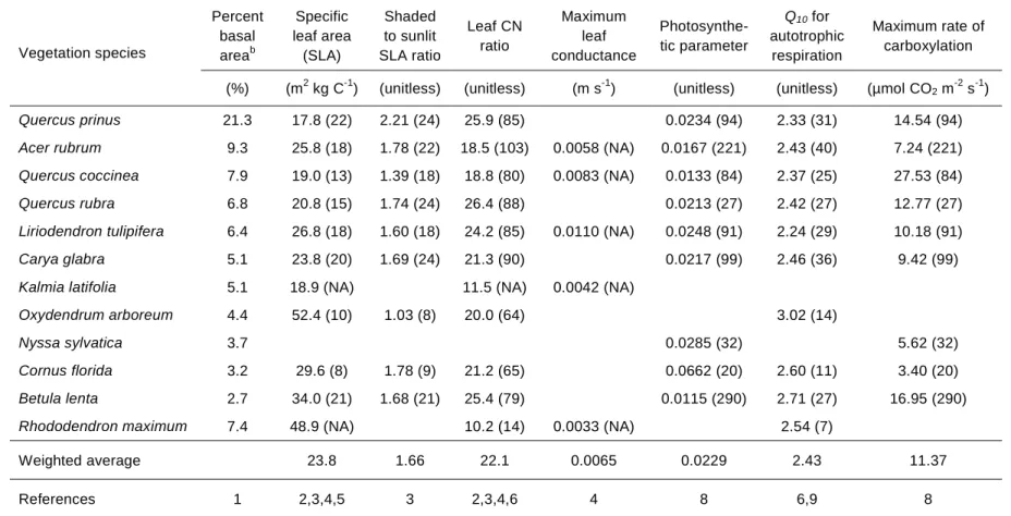
Table 2.2: Species-specific eco-physiologic model parameters

... 32

Table 2.3: Other model parameters ... 34

Table 3.1: Summary of phenological and topographic variables ... 91

Table 3.2: Pearson correlation coefficients between topographic factors and phenological

variables (n = 252) ... 95

Table 3.3: Summaries of multiple regression models (n = 252) ... 97

xiii

LIST OF FIGURES

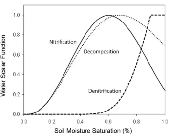
Figure 2.1: Water scalar functions of nitrogen transformation rates as a function of soil

moisture saturation for sandy loam soils; after Parton et al. (1996). ... 23

Figure 2.2: A compartment flow diagram of carbon allocation, transfer, and turnover with

mixed daily and yearly allocation strategies following the current BIOME-BGC

algorithm (Thornton et al. 2002; Thornton 1998). ... 23

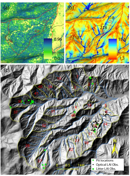
Figure 2.3: Study site (WS18); (a) NDVI (normalized difference vegetation index) from a

June 1, 2003 IKONOS image, (b) wetness index, and (c) locations for WS18 (square),

LAI (leaf area index) measurements, and soil pits within the Coweeta LTER site.

Litter LAI points are from Bolstad et al. (2001). Red and yellow lines represent the

boundaries of watersheds, and dashed lines indicate roads along which artificial gaps

are shown. (a) and (b) are perspective views from the WS18 outlet. The rectangles

within WS18 are three gradient plots (118, 218, and 318). A paired experimental

watershed (WS17) is also shown next to the target watershed where white pines (Pinus

strobus L.) are planted in 1956 after 15-year clear cut periods. ... 25

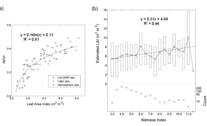
Figure 2.4: (a) A scatter plot between LAI (leaf area index) measurements and NDVI

(normalized difference vegetation index), and (b) hydrologic gradients of estimated

LAI within the study watershed. Litter LAI measurements are from Bolstad et al.

(2001). Circles represent average values, and box plots have lines at the lower quartile,

median, and upper quartile values from each binned group. Counts are the number of

10 × 10 m patches in each group, which are basic units of model simulation. ... 29

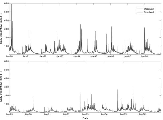
Figure 2.5: Long-term observed and simulated daily streamflow at the study watershed

(1990 ~ 2006), including the 3-year calibration period (October 1999 ~ September

2002). ... 35

xiv

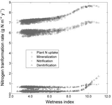
Figure 2.7: Simulated long term (1941 ~ 2005) nitrogen transformation rates (plant

uptake, mineralization, nitrification, and denitrification) in litter and soil as a function

of wetness index. Note that these modeled gradients largely result from in situ N

cycling as lateral transport of mobile nitrogen (nitrate), or organic litter downslope is

not included in the simulation version. Each point represents a 10 × 10 m cell (n =

1253), a basic unit of model simulation. ... 38

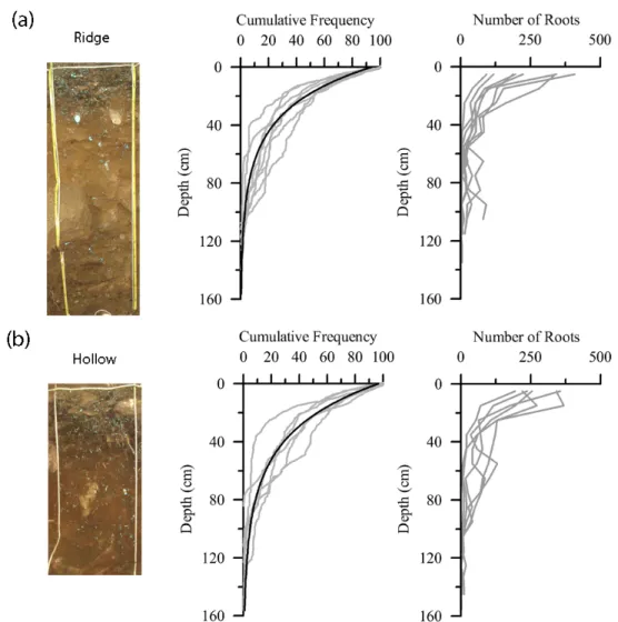
Figure 2.8: The distribution of roots as a function of soil depth for pits located on (a)

ridges and (b) hollows. Distributions are expressed as root cumulative frequency and

as absolute number. Grey lines represent individual pits, while black lines are the

mean of all pits. Photographs are vertical sections of two Q. rubra pits (Table 2.1) dug

within 20 m of each other. Note the difference in the depth of the dark A horizon

between the two sites. Blue painted roots were used for analysis of root distributions.

Modified from Figure 3 in Hales et al. (2009). ... 42

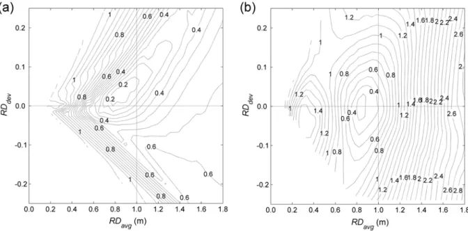
Figure 2.9: Mean absolute error (MAE) of simulated LAI within WS18 over multiple

realizations of average rooting depth (RD

) and spatial pattern of rooting depth

(RD

) under (a) the constant and (b) the alternative allocation strategies. ... 44

Figure 2.10: 3-D and 2-D contour plots of long-term simulated (1941 ~ 2005) average

annual (a) NPP (net primary productivity), (b) ET (evapotranspiration), and (c) WUE

(water used efficiency) over sampled RD

and RD

under constant allocation

strategy. The color bar represents the mean absolute error (MAE) of simulated LAI

(Figure 2.9a). ... 46

Figure 2.11: 3-D and 2-D contour plots of long-term simulated (1941 ~ 2005) average

annual (a) NPP (net primary productivity), (b) ET (evapotranspiration), and (c) WUE

(water used efficiency) over sampled RD

and RD

under alternative allocation

strategy, where allocation ratios are as a function of local rooting depth. The color bar

represents the mean absolute error (MAE) of simulated LAI (Figure 2.9b). ... 47

xv

strategy, while they decrease in proportion to rooting depth under alternative

allocation strategy. Long term patterns of vegetation density (LAI) follow ANPP as a

constant portion of cumulative ANPP is allocated into foliar biomass. ... 48

Figure 3.1: A study site (Coweeta Hydrologic Lab). Grids represent the MODIS

(MOD13Q1; about 230 m) pixels. Red lines represent the boundaries of watersheds.

Letters indicates the pixels for examples of filtering and fitting methods (Figure 3.3;

Figure 3.4). ... 76

Figure 3.2: A typic diagram from Day et al. (1988), which describes vegetation

community types within the study site as a function of slope, aspect, elevation, and

hillslope positions. ... 77

Figure 3.3: Examples of two-step filtering methods from 8-year historical trajectories

(left column) and time-series (right column) of estimated LAI at selected MODIS

pixels ((a) ~ (i); Figure 3.1). Grey and black dots represent filtered values by the

outlier exclusion analysis and the modified BISE methods, respectively. ... 81

Figure 3.4: Examples of the difference logistic function fitting for 8-year estimated LAI

datasets at selected MODIS pixels ((a) ~ (i); Figure 3.1). Vertical dotted lines are

phenological transition dates (t´) from Eq. 3.5. ... 86

Figure 3.5: Analytical solutions of phenological variables; (a) the difference logistic

function, (b) the first derivative, (c) the second derivative (a thick line) and curvature

(grey lines; Eq. 3.4), and (d) the third derivative (a thick line) and the rate of curvature

change (CCR; grey lines). The curvature and CCR curves are drawn with different c

parameter values (0.5 ~ 4.0; Eq. 3.2). The vertical grey lines are analytical solutions

for phenological variables from Eq. 3.5, not changed with different c parameter values.

... 87

xvi

Figure 3.7: Elevational controls on (a) Mid

(grey) and Mid

(black), (b) Length

(grey)

and Length

(black), and (c) LAI

(grey) and LAI

(black). Horizontal error bars

represent Length

and Length

. ... 100

Figure 3.8: Scatter plots of six phenological variables (Mid

, Mid

, Length

, Length

,

LAImin

, and LAI

) between extremely wet (2003, 2005) and dry (2001, 2008) years.

... 101

Figure 3.9: Major topographic controls (elev, taspect) on length phenological variables

(Length

, Length

) between wet (light circles and dashed lines) and dry years (dark

circles and solid line). ... 102

Figure 3.10: Comparison of radiation proxies (taspect, PRR

) from two different

upscaling methods at each MODIS pixels. Radiation proxies of x-axis were calculated

from upscaled DEM at MODIS scale (about 250 m), while those of y-axis from

averaging of the original scale radiation proxies from LIDAR DEM (about 6 m). ... 111

Figure 4.1: A study site (Coweeta Hydrologic Lab). Grids represent the MODIS

(MOD13Q1; about 230 m) pixels. Red and yellow lines represent the boundaries of

sub-watersheds and WS08 (an upper basin of Coweeta). Letters indicates the pixels for

examples of fitting and downscaling methods (Figure 4.2; Figure 4.3; Figure 4.8;

Figure 4.9) ... 130

Figure 4.2: Examples of fitting by the difference logistic function for 8-year MODIS

NDVI datasets (2001 ~ 2008) at selected MODIS pixels ((a) ~ (i); Figure 4.1). ... 140

Figure 4.3: Interannual phenological variations of the fitted MODIS NDVI model at

selected MODIS pixels ((a) ~ (i); Figure 4.1). ... 142

xvii

Figure 4.5: Spatio-temporal patterns of Landsat NDVI values within the Coweeta basin

as a function of DOY. All Landsat TM images are from 2000 to 2008, and absolutely

cloud-free. Points and vertical lines represent an average, and 5th and 95th percentiles

of spatial NDVI values within the WS08 watershed (n = 8654; Figure 4.1). ... 144

Figure 4.6: An example of two downscaling methods on May 5, 2008; (a) a fitted

MODIS FPAR image, (b) a composite Landsat NDVI image, (c) a proportionality

parameter (

α

) map by the simple downscaling method, (d) a downscaled FPAR map

by the simple downscaling method, (e) a potential hourly radiation map (kJ m

h

),

and (f) a downscaled FPAR map by the topographically corrected downscaling

method. ... 147

Figure 4.7: Two examples of the topographically corrected downscaling method on July

1, 2008 (left column) and February 8, 2008 (right column); (a) and (b) fitted MODIS

FPAR images, (c) and (d) composite Landsat TM NDVI images, and (e) and (f)

downscaled FPAR maps. ... 148

Figure 4.8: Examples of the topographically corrected downscaling for the MODIS

FPAR at selected MODIS pixels in 2008 ((a) ~ (i); Figure 4.1). Grey dotted and color

solid lines represent the fitted MODIS FPAR and the downscaled sub-grid FPAR

values respectively. ... 151

Figure 4.9: Examples of the topographically corrected downscaling at selected MODIS

pixels in 2008 ((a) ~ (i); Figure 4.1). Color solid lines represent the downscaled

sub-grid LAI values estimated from downscaled sub-sub-grid FPAR values (Figure 4.8). .... 152

Figure 4.10: A scatter plot between

α

(a proportionality parameter in the

topographically corrected downscaling) and

α

(a proportionality parameter in the

simple downscaling) values on May 5 (cross), February 8 (triangle), and July 1 (circle),

2008. ... 153

Figure 4.11: Temporal patterns of

α

(upper) and

α

(lower) values for a

simulation period (2001 ~ 2008) with 5-day intervals. Points and vertical lines

xviii

Figure 4.12: Observed and simulated daily streamflow at the study watershed (WS08;

Figure 4.1), including the 3-year calibration period (October 2003 ~ September 2006).

... 156

xix

LIST OF ABBREVIATIONS

ANPP

Aboveground Net Primary Productivity

AVHRR

Advanced Very High Resolution Radiometer

BISE

Best Index Slope Extraction

BRDF

Bidirectional Reflectance Distribution Function

CCR

Curvature Change Rate

DBH

Diameter at Breast Height

DEM

Digital Elevation Model

DOS

Dark Object Subtraction

DOY

Day Of Year

ET

Evapotranspiration

EVI

Enhanced Vegetation Index

FPAR

Fraction of absorbed Photosynthetically Active Radiation

GPS

Geographic Positioning System

GSL

Growing Season Length

L1T

Level-one Terrain-corrected

LAI

Leaf Area Index

TM

Thematic Mapper

LIDAR

LIght Detection And Ranging

LTER

Long Term Ecological Research

MAE

Mean Absolute Error

xx

MRT

MODIS Reprojection Tool

NDVI

Normalized Difference Vegetation Index

NPP

Net Primary Productivity

PAR

Photosynthetically Active Radiation

QC

Quality Control

RHESSys

Regional Hydro-Ecological Simulation System

RuBP

Ribulose-BisPhosphate carboxylase-oxygenase

SLA

Specific Leaf Area

SR

Simple Ratio

STARFM

Spatial and Temporal Adaptive Reflectance Fusion Model

UTM

Universal Transverse Mercator

xxi

LIST OF SYMBOLS

A

net rate of leaf photosynthesis

a, b

fitting variables in the logistic function

A

RuBP-limited photosynthesis (an electron transport rate)

APAR

absorbed photosynthetically active radiation per unit leaf area

APARi,t

absorbed PAR at each sub-grid pixel i and date t

Av

Rubisco-limited photosynthesis (a carboxylation rate)

c

difference between fitted maximum and minimum NDVI or LAI

Ci

partial pressure of within leaf CO

CO

atmospheric concentration of carbon dioxide

d

a fitted minimum or background NDVI or LAI value

elev

elevation

FPAR

MODIS FPAR

FPARi,t

FPAR values of sub-grid i on date t

FPARt

MODIS FPAR on date t

g

stomatal conductivity for CO

gs

stomatal conductance for water

gs.max

maximum stomatal conductance for water

g

stomatal conductance for water per unit shaded leaf area

gs.sunlit

stomatal conductance for water per unit sunlit leaf area

i

sub-grid pixel locations

I

effective irradiance

IPARi

potential incident PAR at each sub-grid pixel i

xxii

J

electron transport rate

Jmax

maximum electron transport rate

K

Michaelis-Menten constant of Rubisco for CO

Ko

Michaelis-Menten constant of Rubisco for O

LAI

fitted maximum leaf area index

LAI

fitted minimum leaf area index

LAIshade

total shaded leaf area index

LAIsunlit

total sunlit leaf area index

Lengthoff

length of the senescence period

Lengthon

length of the greenup period

Mid

mid-day of the senescence period

Mid

mid-day of the greenup period

n

number of sub-grid pixels within a single MODIS pixel

NDVI

mean NDVI of NDVI

values within a single MODIS pixel

NDVIi

composite Landsat NDVI at each sub-grid pixel i

NDVIi,DOY

composite Landsat NDVI at each sub-grid pixel i on corresponding DOY

NDVI

lumped NDVI calculated from aggregated radiance at the MODIS scale

NDVIwgt

weighted mean of NDVI

with respect to IPAR

Oi

partial pressure of within leaf O

PRR

potential relative radiation for the whole year

PRRf

potential relative radiation for the senescence season (Oct, Nov)

PRRg

potential relative radiation for the greenup season (Apr, May)

RD

a local rooting depth

Rd

daily leaf respiration

xxiii

t

date

t´

transition dates for phenological signals

taspect

transformed aspect

topidx

wetness index (or topographic index)

V

maximum rate of carboxylation

VPD

vapor pressure deficit

WI

local wetness index

WIavg

average wetness index within the hillslope

α

a proportionality parameter

α

α

of the simple downscaling method

α

α

on date t

α

α

of the simple downscaling method on date t

α

α

of the topographically corrected downscaling method on date t

α

α

of the topographically corrected downscaling method

Γ

CO

-compensation point

θ

sun zenith angle

κ

signed curvature

ψ

soil water potential

Chapter 1

Introduction

1.1

Background

Ecohydrology may be defined as the science which seeks to describe the hydrologic mechanisms that underlie ecologic patterns and processes (Rodriguez-Iturbe 2000). We expand on this definition by including the complementary question of how ecological mechanisms underlie hydrologic patterns and processes, essentially examining the coupled evolution and interactions within ecohydrological systems.

Ecohydrological processes incorporate a very wide variation in temporal scales ranging from sub-daily energy, water, carbon and nutrient flux, to decadal and century level growth and aggradation of ecosystems and biogeochemical development of soils. These processes are interconnected over both time and space by three-dimensional circulation of water through the landscape by the set of dominant surface and subsurface flowpaths, interacting with long term modification of canopy and soil

conditions. Forested watershed responses to climatic patterns involve complex interactions between ecological and hydrological processes (e.g. interception, infiltration, evapotranspiration,

photosynthesis, drainage, succession etc.) mediated by soil moisture dynamics, operating at different temporal and spatial scales. Therefore, spatio-temporal dynamics of soil moisture are key links between hydrologic and biogeochemical processes (Rodriguez-Iturbe 2000).

2

significant bias in model behavior. Especially in topographically complex terrains, prescribing averaged spatial and temporal variations of state variables may underestimate the effect of severe drought due to asymmetric nature of the spatial distribution of soil moisture along with its non-linear control on water and carbon processes (e.g. Band et al. 1993). Given the complexity of these

interactions and their spatio-temporal variations, we must incorporate new observations of ecological and hydrological form and process to reduce the uncertainty related to the state and flux variables in the model. In this process, temporal and spatial resolutions of data assimilation strongly depend on available ecohydrological datasets.

Recent developments in ground based and remote sensing observational technologies, along with coupled distributed ecohydrological modeling paradigms provide the potential to mitigate this problem by linking dynamics measurements with integrated process descriptions. High resolution spatial information (e.g. land cover, topography, canopy cover, soil moisture, precipitation etc.) have aided the development of complex fully distributed models that construct a detailed spatial representation of the variability of the hydrological processes within the watershed. In particular, near real-time global satellite products (MODIS; MODerate Resolution Imaging Spectro-radiometer) enable us to integrate spatio-temporal dynamics of key ecohydrological processes, such as spatio-temporal vegetation dynamics, which are difficult to adequately incorporate in classical lumped hydrological models.

3

These two important biophysical properties are linearly or non-linearly correlated with NDVI (normalized difference vegetation index) from remote sensing images, so the NDVI plays a crucial role in estimating spatio-temporal dynamics of vegetation density from remote sensing images at different scales. In this study, phenological state variables (e.g. FPAR, LAI) are locally estimated within the study area using NDVI values from multi-temporal remotely sensed data (e.g. IKONOS, Landsat TM, MODIS), further evaluated with field measurements.

This dissertation aims to integrate spatio-temporal vegetation dynamics into a distributed

ecohydrological model at different scales, operating over sub-daily to decadal level time scales with specific applications to ecological optimality theory and real-time watershed simulations. Three related questions and topics are addressed within the dissertation papers:

1. To determine if the observed vegetation patterns along hydrologic gradients within a small catchment represent long-term ecohydrologic pattern optimization for carbon uptake (e.g., full system productivity or water use efficiency maximization) at the hillslope scale.

2. To find topography-mediated controls on local vegetation phenology from MODIS NDVI data, and to relate these spatial phenological patterns to micro-climate variations and other factors (e.g. vegetation community types, topographic positions).

3. To develop a downscaling method fusing multi-temporal MODIS-Landsat data in

conjunction with topographic information to produce near real-time estimates of high spatial and temporal resolution canopy phenology in complex terrain, for assimilation into the distributed ecohydrological model.

For the first question, Chapter 2 specifically uses the modeling framework to assess long term development and co-evolution of the ecosystem canopy, soil, and topography. The spatial gradient of vegetation density within a small catchment is estimated with fine-resolution satellite imagery

4

different root depth and allocation strategies as a function of hillslope position. Then, we test whether the simulated spatial pattern of vegetation corresponds to measured canopy patterns and an optimal state relative to a set of ecosystem processes, defined as maximizing ecosystem productivity and water use efficiency at the catchment scale.

In Chapter 3, we develop a robust filtering and fitting method to extract phenological signals from the multi-year trajectories of MODIS NDVI data, and relate spatial patterns of vegetation phenology to topographic factors by a statistical analysis to answer the second question. These topography-mediated phenological patterns are interpreted based on spatial variations of micro-climate and other factors (e.g. vegetation community types, hillslope positions). In particular, scale issues would be examined by comparing these phenological patterns with historical field measurements and interannual variations between very wet and dry years.

For the last question, we develop methods to estimate near real-time vegetation dynamics by downscaling the fitted MODIS FPAR into the Landsat scale with two suggested downscaling methods for the 8-year period (2001 ~ 2008) in Chapter 4. The sub-grid variability of vegetation density within the MODIS pixels is inferred each day from composite NDVI images as a function of day of year assuming they are interannually consistent. Examples of a distributed ecohydrological model are shown assimilating the real-time downscaled vegetation dynamics.

Finally, Chapter 5 summarizes important findings and discusses their further implications.

1.2

A Process-based Distributed Ecohydrological Model

RHESSys (Regional Hydro-Ecological Simulation System) is a GIS-based, ecohydrological

modeling framework designed to simulate carbon, water and nutrient cycling in complex terrain (Band et al. 1993; Tague and Band 2004). One of the unique features of RHESSys is its hierarchical

5

enables the modeling of spatio-temporal interactions between the different ecohydrological processes at the plot to the watershed scale. This approach allows different processes to be affiliated at different spatio-temporal scales and the basic modeling unit to be of arbitrary shape, rather than strictly grid-based.

RHESSys has been developed from several pre-existing models. First, a microclimate model, MT-CLIM (Running et al. 1987) uses topography and user supplied base station information to extrapolate spatially variable climate variables over topographically varying terrain. At the patch level, an eco-physiological model is adapted from BIOME-BGC (Running and Coughlan 1988; Running and Hunt 1993; Kimball et al. 1997) to estimate carbon, water and potential nitrogen fluxes from different canopy cover types, while representation of soil organic matter and nutrient cycling in RHESSys is largely based on CENTURY model (Parton et al. 1993). RHESSys also uses the CENTURYNGAS

(Parton et al. 1996) approach to model nitrogen cycling processes such as nitrification and denitrification (Band et al. 2001). At a hillslope scale, a quasi-distributed hydrological model, TOPMODEL (Beven and Kirkby 1979) is integrated which distributes soil moisture based on the distribution of a topographically defined wetness index.

6

7

Table 1.1: Key processes of RHESSys model

a

computed for sunlit and shaded leaves separately; LAI = leaf area index, T =

temperature,

θ

_{= rootzone soil moisture contents, APAR = absorbed}

photosynthetically active radiation, VPD = vapor pressure deficit, N = nitrogen

contents, C = substrate (carbon) quality, M = substrate (carbon) storage

Processes or Parameters References

Vegetation

Water Interception

Transpiration

Leaf Conductance

f(all-sided LAI)

Penman-Monteith Eq.a

f(T, θ_{, APAR, VPD, CO2)}a _{(Jarvis 1976)}

Carbon Photosynthesis

Maintenance Respiration

Growth Respiration

Allocation / Mortality

Turnover

Farquhar Eq.a (Farquhar et al. 1980)

f(T, N,C)† (Ryan 1991) Constant (Biome-BGC)

Constant (Biome-BGC)

Constant (Biome-BGC)

Nitrogen Stoichiometrically constant C/N ratios for all compartments

Retranslocation of stored nitrogen during the litterfall process

Soil

Water Infiltration

Drainage

Exfiltration / Capillary Rise

Lateral Redistribution

Saturated Throughflow

Phillip’s Eq.

(Clapp and Hornberger 1978)

(Eagleson 1978c)

TOPMODEL (Beven and Kirkby 1979)

TOPMODEL (Beven and Kirkby 1979)

Carbon Decomposition f(T, θ_{, C, M, N) (Parton et al. 1996)}

Nitrogen Mineralization

Denitrification

Leaching

Plant Uptake

f(T, θ_{, M, NH4}+_{) (Parton et al. 1996)}

f(θ_{, M, NO3}-_{) (Parton et al. 1996)}

Flushing hypothesis

8

References

Band LE (1993) Effect of Land-Surface Representation on Forest Water and Carbon Budgets. Journal of Hydrology, 150, 749-772.

Band LE, Mackay DS, Creed IF, Semkin R, Jeffries D (1996) Ecosystem processes at the watershed scale: Sensitivity to potential climate change. Limnology and Oceanography, 41, 928-938. Band LE, Patterson P, Nemani R, Running SW (1993) Forest ecosystem processes at the watershed

scale: incorporating hillslope hydrology. Agricultural and Forest Meteorology, 63, 93-126. Band LE, Peterson DL, Running SW, Coughlan J, Lammers R, Dungan J, Nemani R (1991) Forest

Ecosystem Processes at the Watershed Scale - Basis for Distributed Simulation. Ecological Modelling, 56, 171-196.

Band LE, Tague CL, Groffman P, Belt K (2001) Forest ecosystem processes at the watershed scale: hydrological and ecological controls of nitrogen export. Hydrological Processes, 15, 2013-2028. Baron JS, Hartman MD, Band LE, Lammers RB (2000) Sensitivity of a high-elevation Rocky

Mountain watershed to altered climate and CO2. Water Resources Research, 36, 89-99.

Beven K, Kirkby M (1979) A physically-based variable contributing area model of basin hydrology. Hydrologic Science Bulletin, 24, 43-69.

Christensen L, Tague CL, Baron JS (2008) Spatial patterns of simulated transpiration response to climate variability in a snow dominated mountain ecosystem. Hydrological Processes, 22, 3576-3588.

Clapp RB, Hornberger GM (1978) Empirical equations for some soil hydraulic-properties. Water Resources Research, 14, 601-604.

Creed IF, Band LE (1998) Exploring functional similarity in the export of nitrate-N from forested catchments: A mechanistic modeling approach. Water Resources Research, 34, 3079-3093. Creed IF, Band LE, Foster NW, Morrison IK, Nicolson JA, Semkin RS, Jeffries DS (1996) Regulation

of nitrate-N release from temperate forests: A test of the N flushing hypothesis. Water Resources Research, 32, 3337-3354.

Eagleson PS (1978) Climate, Soil, and Vegetation .3. Simplified Model of Soil-Moisture Movement in Liquid-Phase. Water Resources Research, 14, 722-730.

9

Farquhar GD, Caemmerer SV, Berry JA (1980) A Biochemical-Model of Photosynthetic CO2

Assimilation in Leaves of C3 Species. Planta, 149, 78-90.

Groffman PM, Butterbach-Bahl K, Fulweiler RW, et al (2009) Challenges to incorporating spatially and temporally explicit phenomena (hotspots and hot moments) in denitrification models. Biogeochemistry, 93, 49-77.

Hartman MD, Baron JS, Lammers RB, Cline DW, Band LE, Liston GE, Tague C (1999) Simulations of snow distribution and hydrology in a mountain basin. Water Resources Research, 35, 1587-1603. Hwang T, Band LE, Hales TC (2009) Ecosystem processes at the watershed scale: Extending

optimality theory from plot to catchment. Water Resources Research, 45, W11425.

Hwang T, Kang S, Kim J, Kim Y, Lee D, Band L (2008) Evaluating drought effect on MODIS Gross Primary Production (GPP) with an eco-hydrological model in the mountainous forest, East Asia. Global Change Biology, 14, 1037-1056.

Jarvis PG (1976) The Interpretation of the Variations in Leaf Water Potential and Stomatal

Conductance Found in Canopies in the Field. Philosophical Transactions of the Royal Society of London. Series B, Biological Sciences, 273, 593-610.

Jefferson A, Nolin A, Lewis S, Tague C (2008) Hydrogeologic controls on streamflow sensitivity to climate variation. Hydrological Processes, 22, 4371-4385.

Kimball JS, Thornton PE, White MA, Running SW (1997) Simulating forest productivity and surface-atmosphere carbon exchange in the BOREAS study region. Tree physiology, 17, 589-599. Mackay DS (2001) Evaluation of hydrologic equilibrium in a mountainous watershed: incorporating

forest canopy spatial adjustment to soil biogeochemical processes. Advances in Water Resources, 24, 1211-1227.

Mackay DS, Band LE (1997) Forest ecosystem processes at the watershed scale: dynamic coupling of distributed hydrology and canopy growth. Hydrological Processes, 11, 1197-1217.

Mackay DS, Samanta S, Nemani RR, Band LE (2003) Multi-objective parameter estimation for simulating canopy transpiration in forested watersheds. Journal of Hydrology, 277, 230-247. Meentemeyer RK, Moody A (2002) Distribution of plant life history types in California chaparral: the

role of topographically-determined drought severity. Journal of Vegetation Science, 13, 67-78. Meentemeyer RK, Moody A, Franklin J (2001) Landscape-scale patterns of shrub-species abundance

in California chaparral - The role of topographically mediated resource gradients. Plant Ecology, 156, 19-41.

10

Parton WJ, Mosier AR, Ojima DS, Valentine DW, Schimel DS, Weier K, Kulmala AE (1996) Generalized model for N-2 and N2O production from nitrification and denitrification. Global Biogeochemical Cycles, 10, 401-412.

Parton WJ, Scurlock JMO, Ojima DS, et al (1993) Observations and modeling of biomass and soil organic-matter dynamics for the grassland biome worldwide. Global Biogeochemical Cycles, 7, 785-809.

Rodriguez-Iturbe I (2000) Ecohydrology: A hydrologic perspective of climate-soil-vegetation dynamics. Water Resources Research, 36, 3-9.

Running SW, Hunt ER (1993) Generalization of a Forest Ecosystem Process Model for Other Biomes, BIOME-BCG, and an Application for Global-Scale Models. In: Scaling Physiological Processes: Leaf to Globe (eds Ehleringer JR, Field CB), pp. 141-158. Academic Press Inc., San Diego, CA,

USA.

Running SW, Coughlan JC (1988) A general-model of forest ecosystem processes for regional applications .1. hydrologic balance, canopy gas-exchange and primary production processes. Ecological Modelling, 42, 125-154.

Running SW, Nemani RR, Hungerford RD (1987) Extrapolation of synoptic meteorological data in mountainous terrain and its use for simulating forest evapotranspiration and photosynthesis. Canadian Journal of Forest Research-Revue Canadienne De Recherche Forestiere, 17, 472-483.

Ryan MG (1991) Effects of climate change on plant respiration. Ecological Applications, 1, 157-167. Sanford SE, Creed IF, Tague CL, Beall FD, Buttle JM (2007) Scale-dependence of natural variability

of flow regimes in a forested landscape. Water Resources Research, 43, W08414.

Tague C (2009) Modeling hydrologic controls on denitrification: sensitivity to parameter uncertainty and landscape representation. Biogeochemistry, 93, 79-90.

Tague C, Grant G, Farrell M, Choate J, Jefferson A (2008) Deep groundwater mediates streamflow response to climate warming in the Oregon Cascades. Climatic Change, 86, 189-210.

Tague C, Pohl-Costello M (2008) The Potential Utility of Physically Based Hydrologic Modeling in Ungauged Urban Streams. Annals of the Association of American Geographers, 98, 818-833. Tague C, Seaby L, Hope A (2009) Modeling the eco-hydrologic response of a Mediterranean type

ecosystem to the combined impacts of projected climate change and altered fire frequencies. Climatic Change, 93, 137-155.

11

Thornton PE (2000) User’s Guide for Biome-BGC, Version 4.1.1. Numerical Terradynamic Simulation Group, University of Montana, Missoula, MT, USA.

Chapter 2

Ecosystem processes at the watershed scale: Extending

optimality theory from plot to catchment

2.1

Abstract

The adjustment of local vegetation conditions to limiting soil water by either maximizing productivity or minimizing water stress has been an area of central interest in ecohydrology since Eagleson’s classic study (Eagleson 1978a, 1978b, 1978c, 1978d, 1978e, 1978f, 1978g, 1982; Eagleson and Tellers 1982). This work has typically been limited to consider one-dimensional exchange and cycling within patches and has not incorporated the effects of lateral redistribution of soil moisture, coupled ecosystem carbon and nitrogen cycling, and vegetation allocation processes along topographic gradients. We extend this theory to the hillslope and catchment scale, with in situ and downslope feedbacks between water, carbon and nutrient cycling within a fully transient, distributed model. We explore whether ecosystem patches linked along hydrologic flowpaths as a catena evolve to form an emergent pattern optimized to local climate and topographic conditions. Lateral hydrologic

connectivity of a small catchment is calibrated with streamflow data and further tested with measured soil moisture patterns. Then, the spatial gradient of vegetation density within a small catchment estimated with fine-resolution satellite imagery and field measurements is evaluated with simulated vegetation growth patterns from different root depth and allocation strategies as a function of hillslope position. This is also supported by the correspondence of modeled and field measured spatial patterns of root depths and catchment-level aboveground vegetation productivity. We test whether the

13

relative to a set of ecosystem processes, defined as maximizing ecosystem productivity and water use efficiency at the catchment scale. Optimal carbon uptake ranges show effective compromises between multiple resources (water, light, and nutrients), modulated by vegetation allocation dynamics along hillslope gradient.

2.2

Introduction

Eagleson proposed an elegant optimality hypothesis in water-limited ecosystems (Eagleson 1978a, 1978b, 1978c, 1978d, 1978e, 1978f, 1978g, 1982; Eagleson and Tellers 1982), based on the Darwinian approach that ‘current vegetation composition is an optimal state for productivity’ (Eagleson 2002). In the absence of significant disturbance, natural soil-vegetation systems would co-evolve ‘gradually and synergistically’ with changes in soil structure driven by vegetation to achieve an equilibrium state. Eagleson posited that these equilibria are based on three different optimization strategies at different temporal scales. At short time scales with given climate and soil conditions, minimization of soil water stress produces a vegetation canopy in which steady-state soil moisture will be maximized to minimize vegetation water stress. This short-term equilibrium hypothesis is usually interpreted as a ‘growth-stress trade-off’ (Mackay 2001; Kerkhoff et al. 2004), which conceptually describes the optimal carbon uptake or biomass productivity represented by canopy density in terms of water use. Maximization of biomass productivity is then assumed to control the long-term joint adjustment of vegetation species and soil over successional and quasi-geological time scales respectively. This hypothesis suggests that optimal canopy density in water-limited ecosystems is to be found between minimum water stress and maximum productivity (Rodriguez-Iturbe et al. 1999a).

14

minimization of global water stress through tree/grass coexistence (Rodriguez-Iturbe et al. 1999a, 1999b), emergent optimal water use properties across different biomes (Huxman et al. 2004; Emanuel et al. 2007), and the evaluation of carbon and water fluxes with a short-term physiological optimality

hypothesis (Hari et al. 1999, 2000; Schymanski et al. 2008; van der Tol et al. 2008a, 2008b). In most cases, the adjustment of the canopy to maximize productivity relative to water availability and flux has been evaluated with respect to one dimensional (vertical) water and nutrient exchange at the

ecosystem patch scale, without incorporating lateral moisture redistribution at the landscape scale. Ecohydrological feedbacks between vegetation patterns and lateral water redistribution have been reviewed in various studies, including interactions between surface runoff generation and patterned vegetation (e.g. ‘Tiger bush’) in semiarid ecosystems (e.g. Bromley et al. 1997; Howes and Abrahams 2003; Ludwig et al. 2005; Saco et al. 2007), and feedbacks between groundwater hydrology and vegetation especially in riparian ecosystems (e.g. Camporeale and Ridolfi 2006). Spatial patterns of vegetation are often integrated into hillslope-scale hydrological models to explain the active role of vegetation on local water balance and lateral hydrological processes (e.g. Famiglietti and Wood 1994; Wigmosta et al. 1994; Chen et al. 2005). Mackay (2001) previously evaluated the adjustment of canopy density (leaf area index) to soil moisture and soil nutrients at the hillslope and catchment level, with respect to lateral soil moisture transport.

Determining vertical root profiles and the extent of deep roots has also been a main component of optimality models, as root zone moisture dynamics affect stomatal control on leaf carbon and water exchange, and nitrogen cycling and assimilation (Band et al. 2001; Mackay and Band 1997; Mackay 2001; Rodriguez-Iturbe et al. 1999a; Porporato et al. 2003). Recent studies of optimal rooting

15

Schymanski et al. (2008) introduced a model of root water uptake dynamically optimizing root surface area to meet the canopy water demand while minimizing carbon costs related to the root maintenance. However, the above models do not simulate shifts of allocation strategies and nutrient availability with changing rooting depth or profiles. Increased allocation to deep roots can lead to decreased allocation to foliar biomass and shallow roots, resulting in less light and nutrient availability.

We explore general principles that would explain the tendency to evolve optimal ecosystem

patterns at the hillslope scale, where ecosystem patches exist as part of a drainage chain, or catena, that share some degree of dependency on productivity and resource use with other patches along flowpaths. Optimization has been used to represent a number of different concepts in hydrology and ecology, ranging from maximization of ecosystem functions, to parameter calibrations maximizing model fit to measured runoff. We define optimality here as the maximization of ecosystem functions at the

hillslope or catchment scale, such as net primary productivity, evapotranspiration or water use efficiency. We investigate whether these self organizing canopy patterns have the emergent property of maximizing long term (annual to multi-annual) ecosystem net primary productivity,

evapotranspiration or water use efficiency at the catchment scale, over and above the optimization at individual patches.

16

approach to demonstrate the adjustment of canopy leaf area gradients along hydrologic flowpaths with soil water and nutrient conditions in catchments in central Ontario and California.

In this study, the model is parameterized with detailed measurements in the Coweeta Long Term Ecological Research (LTER) site. The spatial gradient of vegetation density within a small catchment, estimated with fine-resolution satellite imagery and field measurements, is evaluated with simulated vegetation growth patterns from different rooting and allocation strategies. The modeling study will simulate net primary productivity (NPP) and evapotranspiration (ET) for the different range of vegetation patterns. The goal of this modeling study is to determine if the observed patterns of

vegetation density within a small catchment are from long-term ecohydrologic pattern optimization for carbon uptake (e.g. full system productivity or water use efficiency maximization) at the hillslope scale.

2.3

Model overview

This study is based on the use of a process-based ecohydrological model (RHESSys; Regional Hydro-Ecological Simulation System) (Band et al. 1993, 2001; Tague and Band 2004; Mackay and Band 1997) and detailed measurements in the Coweeta LTER site.

2.3.1

A Farquhar photosynthesis model

The concept of ecosystem optimality emerged from eco-physiologists (Cowan and Farquhar 1977; Cowan 1982), who developed theories based on principles stating that a maximum amount of carbon is assimilated for a given amount of water loss. Their theory related the stomatal conductance with photosynthesis using a constant water use efficiency concept for short and long-term regulations (referred to as ‘marginal cost’). The Farquhar photosynthesis model (Farquhar et al. 1980)

17

with respect to water loss (Cowan and Farquhar 1977; Farquhar et al. 2001). Farquhar’s equations for C3 plants are controlled by two rate-determining steps in the photosynthetic reaction: a carboxylation rate (Av) and an electron transport rate (Aj), the minimum of which is the net rate of leaf photosynthesis (A) (Farquhar et al. 1980; de Pury and Farquhar 1997).

d j v A R A

A=min{ , }−

(2.1)

where Rd is daily leaf respiration. In the model, Rd is calculated using reference values at 20 ºC and an empirical relationship between leaf nitrogen content and respiration rate (Ryan 1991). Carboxylation limited photosynthesis (Av) is mediated by Rubisco enzyme, and is referred to as Rubisco-limited

photosynthesis (Farquhar et al. 1980; de Pury and Farquhar 1997; Farquhar and von Caemmerer 1982).

) / 1 ( * max o i c i i v K O K C C V A + + Γ −

=

(2.2)

where Kc and Ko are the Michaelis-Menten constant of Rubisco for CO2 and O2, and Ci and Oi are

partial pressure of within leaf CO2 and O2, and Γ* is the CO2-compensation point. Both K and Γ* are

temperature-dependent usually expressed with reference values at 25 ºC and their increase ratios with 10 ºC increase (Q10 values) (Collatz et al. 1991). Vmax represents the maximum rate of carboxylation, assumed to be a linear relationship with leaf nitrogen content per unit leaf area and Rubisco activity, which includes a temperature-dependent function (de Pury and Farquhar 1997; Chen et al. 1999a; Wilson et al. 2000).

18

4 + Γ

Γ − = i i j C C J

A

(2.3)

where J is the electron transport rate, calculated from a quadratic equation as a function of effective irradiance (Ie) and the maximum electron transport rate (Jmax). A fixed ratio (2.1; Wullschleger 1993) is usually assumed between Jmax and Vmax even though this ratio can vary with temperature sensitivities of both components.

2.3.2

Coupled photosynthesis – stomatal conductance models

Many stomatal conductance (gs) models (e.g. Chen et al. 1999a; Baldocchi et al. 1991; McMurtrie et al. 1992; Sellers et al. 1992; Leuning 1995; Oren and Pataki 2001; Kim et al. 2008) use an

empirical equation from (Jarvis 1976), which assumes that environmental factors act independently to control stomatal conductance.

)

(

)

(

)

(

)

(

.

f

VPD

f

f

APAR

f

CO

g

g

=

ψ

(2.4)

where gs.max is the maximum stomatal conductance for water, f(·) are linear or non-linear scalar functions that evaluate between 0 and 1 for VPD (vapor pressure deficit), ψ (soil water potential), APAR (absorbed photosynthetically active radiation per unit leaf area), and CO2 (atmospheric

concentration of carbon dioxide).

Stomatal conductance is the key link between carbon uptake and water leakage because gas exchange through stomata is usually assumed to be dominated by a diffusion process following concentration gradients under a steady-state assumption (Cowan and Farquhar 1977). Stomatal conductivity for CO2 (gc) can be calculated by dividing the above gs with a constant factor (set to 1.6;

19

vapor and CO2 (Leuning 1995). The rate of CO2 transport across stomata (A) can be expressed as a

function of stomatal conductivity for carbon (gc) and a concentration gradient term (Ca - Ci) (Cowan and Farquhar 1977).

)

(

c

C

C

g

A

=

−

(2.5)

Av from Eq. 2.2 and Aj from Eq. 2.3 can be solved using the quadratic equation, by substituting Ci

from the above equation (Farquhar and von Caemmerer 1982; Chen et al. 1999a). Note that stomatal conductance and photosynthesis are all unit leaf area basis, not unit ground area basis, which would be scaled up with dynamic separation between sunlit and shaded leaves.

2.3.3

Scaling up fluxes from leaves to canopy

Many coupled modeling efforts show that dynamic separation between sunlit and shaded leaves is the most efficient way to represent different rate determining factors for photosynthesis with canopy depth profile without multi-layer simulations (de Pury and Farquhar 1997; Chen et al. 1999a; Wang and Leuning 1998). Following Chen et al. (1999a), total sunlit leaf area index (LAI) (LAIsunlit) is defined as

))

cos

/

5

.

0

exp(

1

(

cos

2

θ

LAI

θ

LAI

=

−

−

Ω

(2.6)

where θ is sun zenith angle, and Ω is the foliage clumping index. Shaded LAI (LAIshade) is LAIshade = LAI - LAIsunlit. Dynamic weighting is applied to calculate canopy-scale stomatal conductance (gs), and

photosynthesis (A) per unit ground area.

shade shade s sunlit sunlit s

s

g

LAI

g

LAI

20

shade shade

sunlit

sunlit

LAI

A

LAI

A

A

=

+

(2.8)

This dynamic separation between sunlit and shaded leaves is justified in that the upper canopy is usually light-saturated whereas the lower canopy responds linearly to irradiance, which should result in a vertical distribution of leaf nitrogen and specific leaf area for their optimal exploitation (Field 1983; de Pury and Farquhar 1997).

2.3.4

Nitrogen limitation

Most temperate forests are limited by nutrients, in particular nitrogen (Vitousek and Howarth 1991; Schimel et al. 1997; Nadelhoffer et al. 1999; Oren et al. 2001). Most ecohydrological catchment models usually incorporate only soil moisture patterns into vegetation dynamics, derived by topographic position, local soil texture, and available rooting depth information without nutrient limitation (Wigmosta et al. 1994; Rodriguez-Iturbe et al. 1999a; Porporato et al. 2002; Ivanov et al. 2008; van der Tol et al. 2008b) and are often applied in strictly water-limited ecosystems.

21

The nitrogen cycle in the model is largely based on the BIOME-BGC model (Running and

Coughlan 1988; Running and Hunt 1993; Kimball et al. 1997; Thornton et al. 2002) for vegetation and the CENTURYNGAS model (Parton et al. 1996) for soil. The model assumes stoichiometrically

constant ratios between carbon and nitrogen (C/N ratio) for all vegetation compartments (leaf, litter, fine root, live wood, and dead wood) and soil pools (Tague and Band 2004). At a daily time step, all soil/litter pools calculate the potential immobilization and decomposition rates based on soil water and temperature. If nitrogen availability cannot satisfy the sum of potential microbial uptake

(immobilization) and plant growth demands (plant uptake), these two demands compete for available soil mineral nitrogen. Plants can also use an internally-recycled nitrogen pool translocated from turnover of leaves and live vegetation parts (stem, coarse root) for remaining demands for nitrogen. Available nitrogen also includes atmospheric deposition, fertilization, or symbiotic/asymbiotic fixation. Detailed explanations are available in the works of Thornton (1998), and Tague and Band (2004).

2.3.5

Allocation

22

Biogeochemical models usually do not simulate actual tree stands which incorporate tree seedling, recruitments, and mortality (Friend et al. 1997). Only total plant mortality is simulated which describe the portion of the plant pools either replaced each year or removed through fire or plant death.

Note that LAI is not prescribed into the model, but the model is self-regulating with respect to LAI based on photosynthate production, respiration, and allocation processes. Optimality models that prescribe aboveground vegetation density and belowground biomass (or rooting depth) usually neglect the feedbacks and constraints of previous, transient carbon, water and nutrient balance. Allocation processes compromise between light, water, and nutrients proportioning fixed carbon into different vegetation compartments based on limiting resources (Tilman 1988; Gedroc et al. 1996;

23

Figure 2.1: Water scalar functions of nitrogen transformation rates as a function of

soil moisture saturation for sandy loam soils; after Parton et al. (1996).

24

2.4

Materials and methods

2.4.1

Site description

The Coweeta Hydrologic Lab is located in western North Carolina and is representative of the Southern Appalachian forest. The Southern Appalachian forest has very diverse flora as a result of combined effect of terrain, microclimate and soil moisture (Whittaker 1956; Day and Monk 1974). Mean monthly temperature varies from 3.6 ºC in January to 20.2 ºC in July. The climate in the Coweeta Basin is classified as marine, humid temperate, and precipitation is relatively even in all seasons; annual precipitation ranges from 1870 mm to 2500 mm with about a 5% increase with 100 m (Swift et al. 1988). The dominant canopy species are oaks and mixed hardwoods including Quercus spp. (oaks), Carya spp. (hickory), Nyssa sylvatica (black gum), Liriodendron tulipifera (yellow poplar), and Tsuga canadensis (eastern hemlock), while major evergreen undergrowth species are Rhododendron maximum (rhododendron) and Kalmia latifolia (mountain laurel) (Day and Monk

25

Figure 2.3: Study site (WS18); (a) NDVI (normalized difference vegetation index)

from a June 1, 2003 IKONOS image, (b) wetness index, and (c) locations for WS18

(square), LAI (leaf area index) measurements, and soil pits within the Coweeta LTER

site. Litter LAI points are from Bolstad et al. (2001). Red and yellow lines represent

the boundaries of watersheds, and dashed lines indicate roads along which artificial

gaps are shown. (a) and (b) are perspective views from the WS18 outlet. The

26

2.4.2

Climate data and historical field measurements

Daily climate (maximum and minimum daily temperature, daily precipitation; CS01/RG06 climate station) and streamflow data (WS18; Coweeta LTER research data ID 3033) are available from 1937, one of the longest hydrological records for forested headwater catchments in the world. For the model simulation, we used universal kriging with elevational trends from 7 points measurements within the Coweeta basin from 1991 to 1995 to develop long-term rainfall isohyets to scale daily precipitation over the terrain.

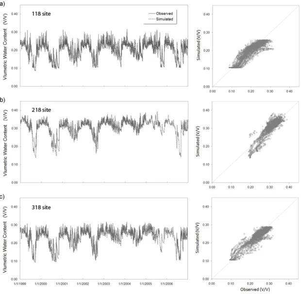
Three LTER research plots have been established along a topographic gradient at high, mid and low catchment positions (118 - xeric, 218 - mesic, and 318 – intermediate) to study ecohydrologic trends within the study watershed (Figure 2.3b), where detailed vegetation, soil and various microclimate data are available. Detailed explanations of these gradient plots are available at the Coweeta LTER homepage (http://coweeta.ecology.uga.edu/gradient_physical.html). We use daily volumetric water content data (Coweeta LTER research data ID 1013) collected with 30-cm CS615 sensors (Water Content Reflectometer, Campbell Scientific Inc., Logan, UT, USA) every 15 minutes from March 1999. At each gradient plot, these TDR sensors are installed at different depths (0 ~ 30 and 30 ~ 60 cm) and at two locations (upper slope and lower slope) within 20 × 40 m original rectangular plots.

Aboveground net primary productivity (ANPP) was estimated from tree ring increments and litterfall measurements in the early 1970’s for the full watershed (Day and Monk 1974, 1977; Day et al. 1988). Biomass increases were estimated from tree ring increments with locally-derived biometric

27

2.4.3

Hydrologic gradients of vegetation density

Leaf area index (LAI), an important carbon state variable in process-based biogeochemical models, is also a valuable driver in the scaling effort as it is well correlated with normalized difference

vegetation index (NDVI) derived from remote sensing images (Nemani et al. 1993; Gholz et al. 1991; Chen and Cihlar 1996; Fassnacht et al. 1997). The NDVI is a normalized ratio between red and near infrared bands.

)

/(

)

(

NDVI

=

ρ

−

ρ

ρ

+

ρ

(2.9)

LAI values were measured at 39 points around the WS18 in early June 2007 using two different methods (Figure 2.3c), with GPS coordinates measured during the previous leaf-off season

(GeoExplorer; Field Data Solutions Inc., Jerome, ID, USA). LAI was measured with an LAI-2000 Plant Canopy Analyzer (LI-COR Inc., Lincoln, NE, USA) using two instruments simultaneously for above and below canopy during overcast sky condition or at dawn or at dusk. Hemispheric images were also taken at the same sites, and analyzed with the Gap Light Analyzer software (Institute of Ecosystem Studies, Millbrook, New York, USA). We also used LAI data estimated from litter biomass and specific leaf area around the Coweeta LTER site (Figure 2.3c), four of which are located within WS18 (Bolstad et al. 2001). These litter-trap measurements are quite valuable in that optical measurements usually do not show much sensitivity in ranges of high leaf area index (Nemani et al. 1993; Fassnacht et al. 1997; Pierce and Running 1988; Gower and Norman 1991).

Spatial patterns of LAI within the watershed were determined from the site-specific correlation between point-measured LAI and NDVI values from a summer IKONOS Image (June 1, 2003; Figure 2.3a) with varying average window size of NDVI pixels and masking from outmost rings in a

28

match between LAI calculations of 0º ~ 23º zenith ranges (1 and 2 rings) and NDVI values by a 3 × 3 averaging window (Figure 2.3a). Considering average canopy height (~ 16 m) within the watershed and 4-meter IKONOS pixel size, this match is quite reasonable in terms of their size correspondences.

Most LAI measurements are located along the regression line except for some outliers (Figure 2.4a), from which we estimated spatial patterns of vegetation density within the target watershed. These outliers are mostly from the sites where thick rhododendron (R. maximum) develops in understory canopy. Dense understory canopy can easily decouple upward ground optical measurements and downward remote sensing images, and also affects NDVI values which are very sensitive to canopy background variations (Huete 1988; Huete et al. 1994).

29

Figure 2.4: (a) A scatter plot between LAI (leaf area index) measurements and NDVI (normalized difference