Smith_unc_0153D_15272.pdf

(1)

MARGINALIZED TWO-PART MODELS FOR SEMICONTINUOUS DATA WITH APPLICATION TO MEDICAL COSTS

Valerie Anne Smith

A dissertation submitted to the faculty at the University of North Carolina at Chapel Hill in partial fulfillment of the requirements for the degree of Doctor of Public Health

in the Department of Biostatistics.

Chapel Hill 2015

Approved by:

John Preisser Brian Neelon Amy Herring Gary Koch

(2)

(3)

ABSTRACT

Valerie Anne Smith: Marginalized Two-part Models for Semicontinuous Data with Application to Medical Costs

(Under the direction of John Preisser and Brian Neelon)

(4)

(5)

To my parents, Larry and Anne Smith, and my grandparents, Hoyte and Myrtle Smith,

(6)

ACKNOWLEDGMENTS

I would like to thank my committee members, Drs. Amy Herring, Gary Koch, and Matthew Maciejewski, for their contributions and helpful comments. Many thanks to my advisors, Drs. Brian Neelon and John Preisser, for introducing me to marginalized models, for all the time spent discussing ideas, and for everything they taught me, both about mod-eling semicontinuous data and writing statistical papers. Thank you to Dr. Gary Koch, for providing invaluable advice, mentoring, and teaching over the past four years. I would also like to thank Drs. Maren Olsen and Matthew Maciejewski, whose support, encouragement, and teaching have been instrumental in developing my skills as a statistician and researcher.

(7)

TABLE OF CONTENTS

LIST OF TABLES . . . x

LIST OF FIGURES . . . xiii

1 LITERATURE REVIEW . . . 1

1.1 Semicontinuous Data . . . 1

1.2 Two-Part Models for Independent Responses . . . 2

1.2.1 Conventional Two-Part Model . . . 2

1.2.2 The Log-Skew-Normal Distribution . . . 3

1.2.3 Parameter Interpretation . . . 5

1.3 Two-Part Models for Clustered Semicontinuous Data . . . 6

1.3.1 Conventional Two-Part Model for Clustered Semicontin-uous Data . . . 6

1.3.2 Extension to Bayesian Modeling . . . 8

1.3.3 Two-Part Population Average Models for Clustered Data . . . 9

1.4 Comparison of One-Part vs. Two-Part Models . . . 11

1.5 Proposed Marginalized Two-Part Model . . . 15

2 A MARGINALIZED TWO-PART MODEL FOR SEMICONTINUOUS DATA . . . 18

2.1 Introduction . . . 18

2.2 Marginalized Two-Part Models for Semicontinuous Data . . . 21

2.2.1 Conventional Two-Part Model . . . 21

2.2.2 Marginalized Two-Part Model . . . 21

2.2.3 Comparison of Treatment Effect Estimates . . . 22

(8)

2.2.5 Extension to the Log-Skew-Normal Distribution . . . 27

2.3 Simulation Study . . . 29

2.4 Analysis of MOVE! Intervention Data . . . 30

2.5 Conclusion . . . 34

3 A MARGINALIZED TWO-PART MODEL FOR LONGITUDINAL SEMICONTINUOUS DATA . . . 41

3.2 Conventional Two-Part Model for Longitudinal Data . . . 43

3.3 Marginalized Two-Part Longitudinal Model . . . 45

3.3.1 Model Specification . . . 45

3.3.2 Subject-Specific and Population Average Interpretations . . . 46

3.4 Parameter Estimation, Computation, and Model Evaluation . . . 47

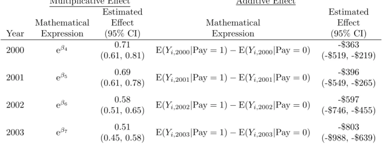
3.5 Analysis of Change in VA Specialty Care Copayment . . . 50

3.6 Conclusion . . . 53

4 COMPARISON OF ONE-PART MODELS AND A TWO-PART MARGINALIZED MODEL FOR THE ANALYSIS OF HEALTH CARE EXPENDITURES . . . 59

4.2 Models Compared . . . 62

4.2.1 MTP Model . . . 63

4.2.2 GLMs Fit with Quasilikelihood . . . 64

4.3 Simulation Details . . . 65

4.3.1 Mean Structure and Properties Examined . . . 65

4.3.2 Simulation 1: Log-Skew-Normal Data . . . 67

4.3.3 Simulation 2: Generalized Gamma Data . . . 67

4.4 Simulation Results . . . 68

4.4.1 Log-Skew-Normal Results . . . 68

(9)

4.4.3 Type I Error Rates . . . 69

4.5 Discussion . . . 70

5 CONCLUSION . . . 79

Appendix A: SAS Code From Chapter 2 . . . 81

Appendix B: Derivation of E(Yij) from Chapter 3 . . . 83

Appendix C: SAS PROC MCMC Code from Chapter 3 . . . 85

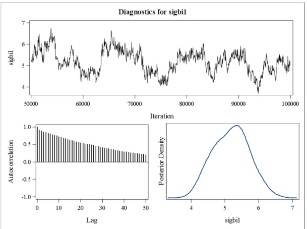
Appendix D: Convergence Diagnostics from Chapter 3 . . . 89

Appendix E: Simulation Details from Chapter 4 . . . 118

(10)

LIST OF TABLES

2.1 Marginalized two-part model performance with 1,000

simula-tions and varying skewness . . . 36

2.2 Means (SD) for MOVE! data . . . 37

2.3 Marginalized two-part model results: MOVE! example . . . 38

2.4 LSN model-estimated means (standard errors) at quartiles of

age, BMI, and DCG Score . . . 39

2.5 Conventional two-part LSN mixture model results: MOVE! example . . . 40

3.1 Descriptive statistics of the matched cohorts in the outpatient

specialty care copay study . . . 56

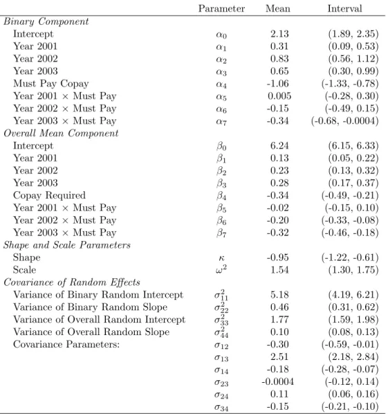
3.2 Posterior means and 95% credible intervals of MTP model parameters . . . . 57

3.3 Model estimated effects of copayment requirement . . . 58

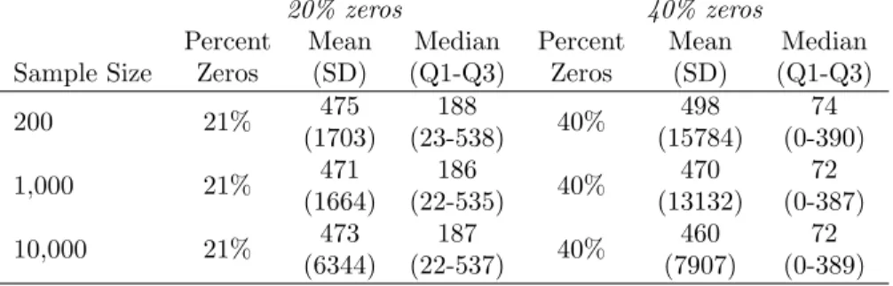
4.1 Descriptive statistics on LSN simulated data . . . 72

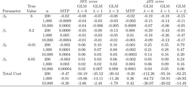
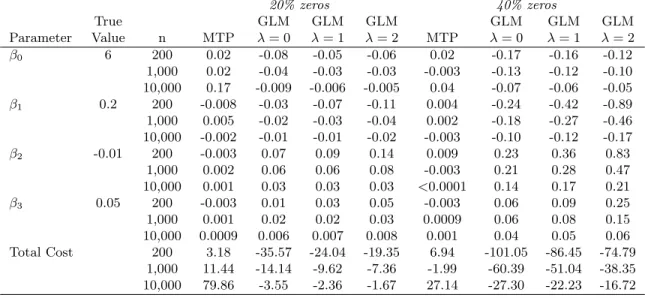
4.2 Median bias of estimated regression coefficients and total cost

predictions in the marginal mean model from LSN data . . . 73

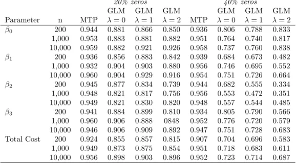
4.3 Coverage of 95% Wald-type confidence intervals for the marginal

mean model parameters and total costs predictions from LSN data . . . 74

4.4 Descriptive statistics on data simulated from the generalized

gamma distribution . . . 75

4.5 Median bias of estimated regression coefficients and total cost

predictions in the marginal mean model from GG data . . . 76

4.6 Coverage of 95% Wald-type confidence intervals for the marginal

mean model parameters and total costs predictions from GG data . . . 77

4.7 Type I error rates at nominal significance level 0.05 for LSN and

GG data . . . 78

E.1 Model performance on independent outcomes of sample size 200 generated from the model in equation (E.1) with κ = 0.5 and

1,000 simulations . . . 119

E.2 Model performance on independent outcomes of sample size 1,000 generated from the model in equation (E.1) with κ = 0.5 and

(11)

E.4 Model performance on independent outcomes of sample size 200

generated from the model in equation (E.1) withκ= 5 and 1,000 simulations 123

E.5 Model performance on independent outcomes of sample size 1,000 generated from the model in equation (E.1) withκ= 5 and 1,000

simulations . . . 124

E.7 Model performance on independent outcomes of sample size 200 generated from the model in equation (E.2) with κ = 0.5 and

E.10 Model performance on independent outcomes of sample size 200

generated from the model in equation (E.2) withκ= 5 and 1,000 simulations 131

E.13 Model performance on independent outcomes of sample size 200 generated from the model in equation (E.3) under the generalized

gamma distribution and 1,000 simulations . . . 135

E.14 Model performance on independent outcomes of sample size 1,000 generated from the model in equation (E.3) under the

general-ized gamma distribution and 1,000 simulations . . . 136

(12)

E.16 Model performance on independent outcomes of sample size 200 generated from the model in equation (E.4) under the generalized

gamma distribution and 1,000 simulations . . . 139

general-ized gamma distribution and 1,000 simulations . . . 140

(13)

LIST OF FIGURES

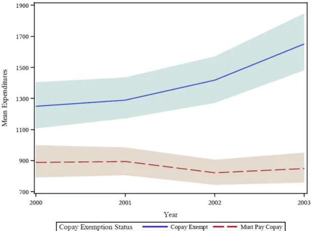
3.1 Model estimated mean expenditures and 95% credible intervals

(shaded regions) for the outpatient specialty care analysis . . . 55

D.1 Convergence diagnostics for α0 . . . 90

D.9 Convergence diagnostics for β0 . . . 98

D.17 Convergence diagnostics for scale parameter, ω2 . . . 106

D.18 Convergence diagnostics for shape parameter, κ . . . 107

D.19 Convergence diagnostics for the random effects covariance pa-rameter,σ11= Var(a1i) . . . 108

D.20 Convergence diagnostics for the random effects covariance pa-rameter,σ22= Var(a2i) . . . 109

D.21 Convergence diagnostics for the random effects covariance pa-rameter,σ33= Var(d1i) . . . 110

D.22 Convergence diagnostics for the random effects covariance pa-rameter,σ44= Var(d2i) . . . 111

(14)

D.24 Convergence diagnostics for the random effects covariance

pa-rameter,σ13= Cov(a1i, d1i) . . . 113

(15)

CHAPTER 1: LITERATURE REVIEW

1.1 Semicontinuous Data

In health services research, it is common to encounter semicontinuous data, such as medical expenditures (Manning et al. 1981; Duan et al. 1983), which are characterized by a point mass at zero followed by a right-skewed continuous distribution with positive support. In the case of medical expenditures, the point mass at zero represents a population of “non-users” who do not receive medical care in a given time interval and therefore have no medical expenditures; the continuous distribution, on the other hand, represents the level of expenditures among health services users given that expenditures were incurred. Considering the two defining components of such outcomes, semicontinuous data can be viewed as arising from two distinct stochastic processes: one governing the occurrence of zeros and the second determining the observed value conditional on it being a nonzero response. The first process is commonly referred to as the “occurrence” or “binary” part of the data, while the second is often termed the “intensity” or “continuous” part. Other examples of semicontinuous outcomes include hospital length of stay (Xie et al. 2004), health assessment scores (Su et al. 2009), and average daily alcohol consumption (Olsen and Schafer 2001; Liu et al. 2012).

(16)

have chosen to model the probability of the outcome being zero separately from the value of the outcome conditional on it being positive in a “two-part” model. Each approach has advantages and disadvantages regarding statistical properties and interpretable results, and often one must compromise on one of these aspects in order to improve the properties of the other.

1.2 Two-Part Models for Independent Responses

1.2.1 Conventional Two-Part Model

There is extensive literature describing two-part mixture models for analyzing semicon-tinuous data. Aitchison (1955) initially highlighted the need for these two defining processes for unbiased estimation in applications involving estimation of expenditures and number of children per household. Deriving semicontinuous counterparts to many commonly used prob-ability distributions, such as the exponential and log-normal, he defined these distributions as a mixture of the binary stochastic process and the continuous positive-valued process con-ditional on observing a positive response. In particular, for the log-normal distribution where the conditionally positive portion of the data follow the density

g(y) = 1

yσp(2π)exp

− 1

2σ2 [ln(y)−µ] 2

, y >0,

he defined the mean and variance of the semicontinuous outcome as

E(Y) = (1−θ) exp

µ+ 1 2σ2

and

Var(Y) = (1−θ) exp(2µ+σ2)exp(σ2)−(1−θ),

whereθ= Pr(Y = 0).

(17)

Duan et al. 1983), as part of the RAND Health Insurance Experiment, introduced the most commonly used two-part model, termed throughout this document as the “conventional” two-part model. For data consisting of independent observations, the generic form of the conventional two-part model can be written as

f(yi) = (1−πi)1(yi=0)×[πig(yi|yi>0)]1(yi>0), yi≥0, i= 1, . . . , n, (1.1)

whereπi = Pr(Yi >0), 1(·) is the indicator function, andg(yi|yi >0) is any density function

applicable to the positive values ofYi, although the log-normal density is often chosen. This

model is parameterized as

η(πi) =zi0α and (1.2)

µi = E(lnYi|Yi>0) =x0iγ. (1.3)

whereη(·) is an appropriate link function, typically a probit or logit function. When fitting this model to independent responses, the binary and conditionally continuous components of the likelihood are separable, and therefore, these two parts are fit separately. The binary component is often modeled using logistic regression, and the continuous component can be fit using standard regression models, such as the log-normal.

1.2.2 The Log-Skew-Normal Distribution

(18)

allowed for varying levels of skewness.

In the case of data that are positively-valued and right-skewed, such as medical expendi-tures, a log transformation can be useful to restrict the range of the predicted original values to the positive scale. Using this transformation, the log-skew-normal density of the positively valued observations becomes

g(yi|yi>0) =

2

ωyi φ

lnyi−ξi ω

Φ

λ

ω(lnyi−ξi)

.

with location parameter ξi, scale parameter ω > 0, and shape parameter λ, all on the log

scale, and whereφ(·) is the probability density function and Φ(·) is the cumulative distribution function for the standard normal distribution.

Chai and Bailey (2008) showed the superior performance of the log-skew-normal (LSN) distribution compared to a log-normal distribution when conducting inference on the positive continuous part of positively skewed semicontinuous data. They additionally highlighted that the log-normal distribution is a special case of the LSN distribution, whenλ= 0, so the appropriateness of the LSN vs. log-normal distribution can be assessed via a likelihood ratio test.

(19)

1.2.3 Parameter Interpretation

Because they explicitly accommodate both data generating processes, two-part mixture models are an ideal choice for modeling semicontinuous data. Regardless of the distribution used, however, covariates in the second, or continuous, part of such two-part models are interpreted conditionally upon having observed a positive outcome. Consequently, attempts to combine these two parts to form the overall marginal mean effect of any covariate relies on specifying values for each of the other covariates in the model. As such, it is generally challenging to obtain a straightforward interpretation of covariate effects on the marginal mean in two-part models.

In many cases, however, investigators’ main interest lies in examining such effects on the marginal mean in order to draw conclusions about the impact of predictors on the population as a whole. For example, in economic studies of system-wide health care expenditures, inves-tigators and policy makers may wish to understand the average effect on medical expenditures of increasing specialty care copayments (Maciejewski et al. 2012a) or of bariatric surgery for weight loss (Maciejewski et al. 2010b; 2012b) on the entire affected or eligible populations rather than estimating separate effects for the probability of incurring expenditures and the level of expenditures given that any are incurred. In particular, an intervention may have one effect on the probability of occurrence but the opposite effect on the intensity given occur-rence. In such cases, policy makers may be left without a true understanding of the overall population-level effect of such an intervention.

(20)

1.3 Two-Part Models for Clustered Semicontinuous Data

Clustered semicontinuous data arise from many situations. In the example of medical expenditures, analysts may be interested in trajectories of a population’s expenditures on health care over several years, or alternatively, may be interested in expenditures on pre-scription drugs incurred by patients clustered within physicians (Zhang et al. 2006). All of the issues related to model estimation of cross-sectional semicontinuous data are relevant to clustered semicontinuous outcomes as well. However, there are additional complications and considerations with clustered outcomes. As with any clustered outcome, the model estima-tion approach needs to incorporate the correlaestima-tion of repeated measurements in addiestima-tion to accounting for missing data due to loss of follow-up or death. Furthermore, in the case of lon-gitudinal data, the distribution of lonlon-gitudinal outcomes, and in particular, the proportion of zeros, is dependent upon the length of time interval under consideration. In many situations, particularly with health expenditures, the longer the time interval, the smaller the proportion of observed zeros in the expenditure distribution.

1.3.1 Conventional Two-Part Model for Clustered Semicontinuous Data

Olsen and Schafer (2001) first extended two-part models to longitudinal data. They proposed a logistic regression model with random effects for the binary part of the data combined with a linear mixed effects model for the log of the conditionally positive part and assumed that the random effects from these two models were jointly normally distributed and possibly correlated. This allowed the probability of occurrence at one time point to be associated with the level of the outcome given occurrence at another time point. Such a model can take the notation

logit(πi) =Xiα+Zici and (1.4)

µi = E(lnYi|Yi >0) =Xi∗γ+Z ∗

(21)

with

bi =

   ci di  

∼N



 0,Ψ =



 

Ψcc Ψcd

Ψdc Ψdd

     

Olsen and Schafer suggested a Laplace approximation with a Fisher scoring algorithm to obtain maximum likelihood estimates, and illustrated their model using data from a longitu-dinal study of middle and high school students on alcohol use. They additionally conducted a simulation study showing low bias and good coverage probabilities for the parameter estimates of both the fixed effects and variance components.

Tooze et al. (2002) proposed a very similar two-part model with correlated random effects, utilizing quasi-Newton optimization of the likelihood approximated by Gaussian quadrature rather than a Laplace approximation. This provided the ability to fit the model in standard statistical software packages, such as SAS (SAS Institute, Cary, NC), and they provided a SAS macro that calls procedures GENMOD and NLMIXED to fit such models. Rather than illustrating their model on a longitudinal data set as in Olsen and Schafer, they provided an example of its use for cross-sectional medical expenditure data that was clustered by house-hold. Their method, however, could also be applied to longitudinal repeated measurements data.

The models proposed by Olsen and Schafer and Tooze et al. both account for potential correlation between the binary and continuous parts of the data. If, however, the occurrence and intensity are uncorrelated, the likelihoods are separable and thus each can be fit separately by maximum likelihood methods. This independence assumption can be very attractive as the inclusion of correlated random effects can introduce severe computational difficulties, at times so extreme that it may not even be possible to fit such a model. However, in many situations, it is quite reasonable to believe that the probability of occurrence, such as having any medical expenditures, at one time point may be related to the intensity, such as level of expenditures, at another time point. For example, patients who are more likely to incur expenditures may also have higher expenditures when they are incurred.

(22)

be-tween the binary and continuous parts of the model. Because the second part of a conventional two-part model includes only those who had a positive outcome, bias from informative clus-ter sizes arises as parameclus-ters in the binary part of the model influence the clusclus-ter size in the continuous part of the model. For example, if those who are more likely to have a positive outcome are also more likely to have a higher level of the outcome given occurrence, then higher levels of the outcome will be over sampled in the continuous model. Su et al. showed that an incorrect assumption of independence between the occurrence and intensity models can produce bias in the estimation of both the regression coefficients and variance components in the continuous part of the model. Further, the direction and size of this bias for most of the estimates relies on true values of the other parameters, including variance components, in both parts of the model. As such, it can be difficult to quantify in a general pattern.

Since the introduction of the correlated, longitudinal two-part model, others have extended it to additional situations. For example, Liu et al. (2008a) incorporated four parts rather than two parts, modeling separately the probability of incurring inpatient and outpatient expenditures and the level of each given they were incurred. In a different manuscript, Liu et al. (2008b) also extended two-part models to multi-level models, incorporating a third level of clustering and correlated random effects. The correlated, longitudinal model thus provides a strong foundation from which many more flexible models can be adapted, although complicated model structures can at times be hampered by computational challenges.

1.3.2 Extension to Bayesian Modeling

(23)

two-part hierarchical model. They fit nearly the same underlying model as Olsen and Schafer, but replaced the logit link function in the binary part with a probit link function for compu-tational simplicity. Using non-informative prior distributions and Markov Chain Monte Carlo (MCMC) sampling, they used this two-part model to examine physician- and patient-level patterns in pharmaceutical expenditures among patients clustered within physician.

Similarly, Cooper et al. (2007) applied two-part models to longitudinal data, using Gibbs sampling MCMC methods and ‘vague’ prior distributions to analyze health care costs over time among individuals with early inflammatory polyarthritis. They compared the results of four models, including both one-part and two-part models, with varying specifications of random effects and distributional assumptions.

Bayesian approaches have been proposed for other extensions to two-part models as well. Ghosh and Albert (2009) developed a two-part model using penalized splines to model the effect of time and the time by treatment interaction. They fit their model using Gibbs sampling MCMC methods and illustrated it by analyzing clinical trial data on acupuncture for treating chemotherapy-induced vomiting in breast cancer patients. Additionally, Neelon et al. (2011) developed a Bayesian two-part growth mixture model to characterize the effect of increased mental health and substance abuse benefits in the Federal Employee Health Benefits Program on mental health use and expenditures. They used an MCMC algorithm to fit a two-part latent class model under weakly informative prior distributions for all parameters, and provided a simulation study showing low bias for all parameter estimates and good coverage rates for the 95% credible intervals. In short, Bayesian approaches to fitting a wide array of two-part models have been shown to maintain good statistical properties while providing computational simplicity and flexibility.

1.3.3 Two-Part Population Average Models for Clustered Data

(24)

param-eter estimates differ in magnitude from their population average counterparts (Diggle et al. 2002). Most work in two-part model marginalization has been with regard to marginalizing over the random effects, converting subject-specific parameter estimates into population av-erage estimates. Hall and Zhang (2004) proposed one such method for obtaining population average parameter estimates from zero-inflated models, utilizing an expectation solution (ES) algorithm, a generalization of the EM algorithm. This algorithm used generalized estimating equations (GEEs) in the S-step to estimate population average covariate effects while ac-counting for correlation within clusters. They applied their algorithm to several zero-inflated models, including zero-inflated Poisson, zero-inflated negative binomial, and zero-inflated cen-sored log-normal models, in which they assumed that some zeros were true zeros and some were small positive values that were censored. However, due to the complexity of their algo-rithm, such estimation is not available in standard statistical software and therefore has not been widely implemented in practice.

Su et al. (2011) proposed a likelihood-based population average model for longitudinal semicontinuous data. Assuming a bridge distribution for the binary random intercept, as opposed to the ordinary normal distribution assumption, they provided a simple formula for converting the subject-specific binary parameter estimates into population average estimates based on an estimated parameter of the bridge distribution. Although later corrected, they incorrectly assumed that the continuous model would provide population average parameter estimates on the log scale due to using a linear mixed model with an identity link. In a correction, however, Tom et al. (2013) showed that, when correlation exists between the binary and continuous parts of the model, the population average parameter estimate is no longer equivalent to the subject-specific estimate when using an identity link. While there is no closed form for the conversion between subject-specific and population average parameter estimates in such scenarios, they provided mathematical bounds for the difference and suggested numerical techniques to calculate the conversion. Tom et al. also suggested marginalizing over the two parts of the two-part model to obtain estimates of the overall marginal mean, E(Yij), when the outcome variable was log-transformed. A closed form was

(25)

lie and again suggested numerical evaluation.

As with independent data, an investigator’s main interest often lies in examining covariate effects on the marginal overall mean, E(Yij), in order to draw relevant policy conclusions about

the impact of predictors on the population as a whole after accounting for clustering. While Tom et al. preliminarily addressed methods to calculate the overall mean, E(Yij), under a

log-transformation, their method did not estimate covariate effects on the overall mean. None of the two-part models for semicontinuous data provided in the literature provide parameter estimates that allow easy and interpretable estimation of such effects.

In the zero-inflated count literature, however, Long et al. (2014) proposed a marginalized model for zero-inflated Poisson (ZIP) regression. They parameterized their model in a two-part formulation, with the first two-part modeling the probability of an observation being a zero observed in excess of what is expected from a Poisson distribution. In the second part, they parameterized the model in terms of the overall mean, combining excess zeros with the Poisson-generated data. Utilizing this parameterization within the ZIP likelihood framework, they accounted for the zero-inflated nature of the data while also providing estimates of covariate effects on the overall mean, marginalized over the excess zeros in the distribution. Through several simulation studies, they showed low bias and good coverage probabilities for the model parameters and showed that, particularly in the presence of highly skewed covariates, their model out-performed standard Poisson regression and ZIP regression models. Illustrating their method with data from an intervention designed to reduce the number of risky sexual behaviors, they obtained an incidence density ratio for the intervention effect that was easily interpretable as the effect on the overall population mean number of risky sexual encounters. Hereafter, in this proposal, the term “two-part model” refers to two-part models for semicontinuous data rather than count data.

1.4 Comparison of One-Part vs. Two-Part Models

(26)

effects of covariates on the overall marginal mean of both users and non-users, a quantity often of primary interest to investigators. Rather, two-part models provide estimates of covariate effects on the probability of having a positive outcome and on the level of the outcome conditional upon it being positive. The conventional two-part model thus may not be ideal for an analyst wishing to estimate the effect of covariates on the overall marginal mean. One-part models, on the other hand, incorporate both the zero and positively continuous values as arising from the same stochastic process and permit interpretation of covariate effects on the overall mean. One-part models typically take one of two general forms. In one form, a small constant is added to the outcome to ensure all values are positive and the outcome is then transformed to minimize skewness. Most commonly, the log transform is used. Alternatively, a generalized linear model (GLM) can be utilized, often with a log link, to avoid transformation and the need to add a constant to all values. Because these models allow simpler computation and interpretation, it is therefore of interest to question whether one-part models may be possible to use for semicontinuous data without creating bias or sacrificing too much precision.

(27)

and precise. Using a split-sample analysis for cross validation and comparing mean squared forecast error among the models, they found that the two-part and four-part models were indistinguishable while performing significantly better than their one-part counterpart and the ANOVA and ANOCOVA models. Ultimately, they recommended the four-part model when needing to assess inpatient expenses in an analysis.

(28)

Mullahy (1998) emphasized the need for analysts to consider their modeling approach when inferences on E(y|x) are of primary interest. In particular, he focused on two main issues that arise in such two-part models: removing the conditioning ony >0 and re-transforming from lny to y. Emphasizing that re-transformation, and thus inferences on E(y|x), can be greatly biased if the model error term is dependent on the covariates, he advocated consid-eration of a modified two-part model, specified as E(y|y > 0,x) = exp(xβM) or a one-part

exponential conditional mean (ECM) model, specified as E(y|x) = exp(xζ). Analyzing the number of doctor visits in a 12 month period among 36,111 individuals ages 25 to 64, which included 23.6% having zero visits, he examined the performance of the ECM model, fit via non-linear least squares, compared to the conventional and modified two-part models. He found that parameter estimates were quite similar among the models and conjectured that larger differences may be found in a sample with a larger proportion of zero values. Examin-ing mean prediction error (MPE) and mean squared error (MSE), he found that the modified two-part model performed slightly better than the ECM model, and both performed better than the conventional two-part model.

(29)

variance, and the one-part GLM with variance proportional to the mean. Ultimately, they recommended that researchers not specifically interested in the probability of use begin by fitting one-part models citing that zero observations can be included in such models without difficulty. If the probability of use were of specific interest, or if the researcher were unable to find a suitably fitting one-part model, they then suggested proceeding to examine two-part models.

Cooper et al. (2007) extended this comparison to a longitudinal setting, comparing four models to predict the costs incurred over time by individuals with inflammatory polyarthritis. Using a Bayesian perspective with vague priors and Gibbs sampling MCMC methods, they compared two one-part log-normal models, one with a random intercept only and one with a random intercept and slope for year, and two two-part models. The one-part models used log-transformed expenditures as the outcome with $1 added to ensure positive values. The two-part models both used logistic regression with a random intercept for the first part, and the second parts were a log-normal model with random intercept and slope for year and a gamma regression with log link, also including a random intercept and slope. The models were fit to a random sample of 76% of the data, and the remaining 24% was used to assess the predictive abilities of the models. In the 76% learning sample, the percentage of individuals with zero expenditures ranged from 32% to 54% over the years of the study. The models were also compared using the Bayesian Deviance Information Criterion (DIC). Under both of these criteria, the two-part models compared favorably to the one-part models.

Given the mixed conclusions from prior literature, there is no clear solution as to under what scenarios one-part models may provide a suitable alternative to their two-part counter-parts when one’s goal is to make inferences regarding the effect of covariates on the overall marginal mean of semicontinuous data.

1.5 Proposed Marginalized Two-Part Model

(30)

appropriately account for the unique statistical properties of semicontinuous data, but on the other, investigators need model estimates that are interpretable for their policy questions of interest. Previously, methods have not existed that simultaneously accounted for the excess zeros and skewness while also providing easily interpretable estimates of covariate effects on the overall marginal mean, E(Y).

This dissertation develops a new marginalized two-part (MTP) model that overcomes many of the drawbacks of previous approaches, including difficulty in interpreting covariate effects on the overall mean, a target of primary interest in many studies. Rather than param-eterizing the model in terms of the mean of the transformed, conditionally positive outcomes in the second part, the MTP model parameterizes covariate effects directly on the overall mean, E(Y), on the untransformed scale. This allows parameter estimates to be interpreted as the multiplicative effect on the overall mean rather than on the conditional mean of only the positive outcomes. Our approach also has the advantage of providing estimates of co-variate effects on the probability of incurring a positive-valued outcome, as in the first part of two-part models, as well as accounting for the zero-inflated and skewed nature of many semicontinuous outcomes.

We extend the MTP model to longitudinal or clustered data via the inclusion of random effects. This model can be fit using maximum likelihood or Bayesian approaches, although we propose the latter to increase flexibility and overcome computational difficulties when model-ing complex random effect structures. This approach provides easily computed predictions of the overall mean outcome, and the parameter interpretations obtained from the MTP model provide the same simple interpretation as those from the one-part GLMs without sacrificing statistical appropriateness. Thus, the MTP model can provide useful policy conclusions while remaining rooted in good statistical practice.

(31)

With such trade-offs, it is natural to question under what conditions each modeling approach exhibits better performance. Assessing bias, test size, and coverage of nominal 95% confidence intervals for covariate effects and model predictions, we fit these models to data generated under varying distributions, proportion of zeros, and sample sizes to inform under what scenarios the models are appropriate and when they encounter difficulties.

(32)

CHAPTER 2: A MARGINALIZED TWO-PART MODEL FOR SEMICONTINUOUS DATA1

2.1 Introduction

In health services research, it is common to encounter semicontinuous data, such as medical expenditures (Manning et al. 1981; Duan et al. 1983), which are characterized by a point mass at zero followed by a right-skewed continuous distribution with positive support. In the case of medical expenditures, the point mass at zero represents a population of “non-users” who do not receive medical care in a given time interval and therefore have no medical expenditures; the continuous distribution, on the other hand, represents the level of expenditures among health services users given that expenditures were incurred. Considering the two defining components of such outcomes, semicontinuous data can be viewed as arising from two distinct stochastic processes: one governing the occurrence of zeros and the second determining the observed value conditional on it being a nonzero response. The first process is commonly referred to as the “occurrence” or “binary” part of the data, while the second is often termed the “intensity” or “continuous” part. Other examples of semicontinuous outcomes include hospital length of stay (Xie et al. 2004), health assessment scores (Su et al. 2009), and average daily alcohol consumption (Olsen and Schafer 2001; Liu et al. 2012).

There is extensive literature describing two-part mixture models for analyzing semicon-tinuous data. Aitchison (1955) initially highlighted the need for these two defining processes for unbiased estimation in applications involving estimation of expenditures and number of children per household. Deriving semicontinuous counterparts to many commonly used prob-ability distributions, he defined these distributions as a mixture of the binary stochastic

1_{This chapter previously appeared as an article in Statistics in Medicine. The original citation is as follows:}

(33)

process and the continuous positive-valued process conditional on observing a positive re-sponse. Cragg (1971), Manning and Duan (Manning et al. 1981; Duan et al. 1983), and others extended this approach to the regression setting, modeling the binary and continuous components as functions of covariates. Most commonly, the binary part is modeled via lo-gistic regression and the continuous component via a log-normal model. However, because the log-normal distribution imposes a sometimes unrealistic condition of symmetry on the log-scale, alternative distributions such as the log-skew-normal have recently been proposed for the continuous part in an effort to relax these somewhat restrictive assumptions (Azzalini 1985; Chai and Bailey 2008). More recent extensions include incorporating longitudinal data (Olsen and Schafer 2001; Tooze et al. 2002), assessing bias (Su et al. 2009), and examining alternative data transformations (Mullahy 1998).

Because they explicitly accommodate both data generating processes, two-part mixture models are an ideal choice for modeling semicontinuous data. When adjusting for covariates, these models typically include one set of parameters for the binary response and a second set for the continuous component conditional on a positive response. In particular, covariates in the second, or continuous, part are interpreted conditionally upon having observed a positive outcome. Consequently, attempts to combine these two parts to form the overall marginal mean effect of any covariate relies on specifying values for each of the other covariates in the model. As such, it is generally challenging to obtain a straightforward interpretation of covariate effects on the marginal mean in two-part models.

(34)

effect on the probability of occurrence but the opposite effect on the intensity given occur-rence. In such cases, policy makers may be left without a true understanding of the overall population-level effect of such an intervention.

To achieve more interpretable effects, Mullahy (1998) and Buntin and Zaslavsky (2004) propose using a one-part exponential conditional mean model to estimate effects of covariates on the marginal mean. While this one-part model provides interpretable estimates, it does not explicitly account for the zero-inflated nature of the data or provide investigators with estimates of covariate effects on the probability of occurrence. Thus, alternative models must be considered when interest lies in estimating both the binary component and the overall marginal mean.

We propose a new “marginalized” two-part model for semicontinuous data which yields more interpretable effect estimates in two-part models by parameterizing the model in terms of the marginal mean. This model maintains many of the important features of conventional two-part models, such as capturing zero-inflation and skewness, but allows investigators to examine covariate effects on the overall marginal mean, a target of primary interest in many applications. We also propose an extension to accommodate log-skew-normal data to relax the commonly used log-normal assumption for the continuous part of the model. We illustrate the approach by evaluating the effect of a behavioral weight loss intervention on health care expenditures in the Veterans Affairs (VA) health care system.

(35)

2.2 Marginalized Two-Part Models for Semicontinuous Data

2.2.1 Conventional Two-Part Model

We begin with a review of the conventional two-part model presented in Cragg (1971), Manning and Duan (Manning et al. 1981; Duan et al. 1983) and elsewhere. For data consisting of independent observations, the generic form of the conventional two-part model can be written as

f(yi) = (1−πi)1(yi=0)×[πig(yi|yi>0)]1(yi>0), yi≥0, i= 1, . . . , n, (2.1)

whereπi = Pr(Yi >0), 1(·) is the indicator function, andg(yi|yi >0) is any density function

applicable to the positive values ofYi, although the log-normal density is often chosen. This

model is parameterized as

logit(πi) =zi0α and (2.2)

µi = E(lnYi|Yi>0) =x0iγ. (2.3)

When fitting this model to independent responses, the binary and conditionally continuous components of the likelihood are separable, and therefore, these two parts are fit separately. The binary component is often modeled using logistic regression, and the continuous compo-nent can be fit using standard regression models, such as the log-normal.

2.2.2 Marginalized Two-Part Model

To obtain interpretable covariate effects on the marginal mean, we propose the following

(36)

two-part (MTP) model specifies the linear predictors

logit(πi) =z0iα and (2.4)

E(Yi) =νi= exp(x0iβ). (2.5)

Parameter estimates can be obtained using standard optimization routines such as Newton-Raphson or Fisher scoring. Model-predicted means and standard errors can also be easily obtained under this parameterization in a single step by estimating exp(x0_iβ) at the desired values of the covariates.

2.2.3 Comparison of Treatment Effect Estimates

Using the conventional model shown in equation (2.3), γj is interpreted as the effect of a

unit increase in thejth covariate, xij, on the conditional mean of ln(Yi) given Yi is positive.

In many applications, however, this interpretation has limited usefulness as it is only relevant for the population of health services users. Rather, interest often lies in estimating the effect of covariates xi on the marginal mean of Yi for the combined population of health services

users and non-users; that is the effect of xi on E(Yi) unconditionally. In the case of the

log-normal distribution, that is the effect ofxi on

E(Yi) =νi=πiexp(µi+σ2/2) =

ez0iα 1 + ez0iα

exp(x0_iγ+σ2/2), (2.6)

whereσ2 is the variance ofYi on the log scale. Assuming xi =zi, as is commonly specified,

it follows from (2.6) that the per-unit effect of thej-th covariate,xij, on the marginal mean

is

E(Yi|xij =j+ 1,x˜i)

E(Yi|xij =j,x˜i)

= 1 + exp [ ˜xi

0_α_˜₊_α j·j]

1 + exp [ ˜xi0α˜ +αj·(j+ 1)]

exp(αj +γj), (2.7)

(37)

specify fixed values for the remaining covariates in order to obtain a marginal interpretation for the effect ofxij. Further, to obtain confidence intervals or formal inference on this marginal

effect, the delta method or resampling techniques must be employed.

Using the MTP model as parameterized in equation (2.5), β is estimated for the entire population as opposed to γ, which is conditional on Yi > 0. Unlike γj in the conventional

model, exp(βj) can be interpreted as the multiplicative effect on the unconditional marginal

mean, νi, when covariate xij increases by one unit. In other words, the left-hand-side of

(2.7) equals exp(βj) under model (2.5). Unlike the conventional model, standard errors and

confidence intervals for covariate effects on the marginal mean are easily obtained as part of the standard model output.

There are other important distinctions between the models. In particular, when the model includes ancillary covariates with no interactions, the MTP model assumes a homogeneous treatment effect on E(Yi) whereas the conventional model yields heterogeneous effects that

depend on the specific values of the additional covariates, potentially creating misleading results. As an illustrative example, we generated a simulated dataset of sample size 10,000 using the following specification:

logit(πi) =α0+α1xi1+α2xi2 and

E(Yi) =νi = exp(β0+β1xi1+β2xi2),

wherexi1 ∼N(50,100) andxi2 ∼Bernoulli(0.5). We specified parameters values asα0= 14.4,

α1 = −0.3, α2 = 1.6, β0 = 5, β1 = 0.05, and β2 = 1.1 and assumed Yi followed the

(38)

third quartiles of xi1, taking values 43, 50, and 57, respectively. Under the conventional model, the estimated effects of an increase in xi2 on E(Yi) were multiplicative increases of

2.5, 4.4, and 8.3, respectively, while the true multiplicative increase was 3.0 regardless of the value of xi1. It is worth pointing out that when treatment effect heterogeneity truly exists, the MTP model can accommodate this through the systematic inclusion of interactions, which should be driven by subject-matter considerations. While the conventional model also accommodates the systematic inclusion of subject-matter driven interactions, it imposes an arbitrary heterogeneity that always exists unless one omits the treatment covariate from the binary part of the model.

(39)

using the MTP model, however, estimation of the treatment effect does not require averag-ing over the observed values of the other covariates in the sample; therefore, these estimates provide much greater generalizability and ease of computation.

This is not to say that the MTP model should be preferred over the conventional model in all cases. Indeed, when the primary target of inference is E(Yi|Yi > 0), the MTP model

engenders arbitrary heterogeneity and provides less interpretable estimates on the conditional mean ofY among the positive values. Ultimately, the choice between models should be guided by the aims of the analyst. If the aim is to model treatment effects on E(Yi) in the presence

of confounders, one should use the MTP model; on the other hand, if the target of inference is E(Yi|Yi >0), the conventional model should be used.

2.2.4 Marginalized Two-Part Log-Normal Model

When modeling semicontinuous data, the continuous component is most frequently mod-eled using a log-normal distribution. The generic form of the two-part log-normal model for independent responses can be written as in (2.1) with g(yi|yi > 0) taking the log-normal

density function LN(·;µ, σ2) with mean µ and variance σ2 on the log scale. The marginal mean and variance ofYi are then given by (Aitchison 1955):

E(Yi) =νi =πiexp(µi+σ2/2) and (2.8)

Var(Yi) =πiexp(2µi+σ2)

exp(σ2)−πi

. (2.9)

The likelihood, parameterized in terms of πi andµi, is:

L(π,µ|y) =Y

i

(1−πi)1(yi=0)

πi yi

√

2πσexp

− 1

2σ2(lnyi−µi) 2

1(_yi>0)

.

(40)

(2.8) can be rearranged to solve forµi, yielding

µi = lnνi−lnπi−σ2/2

=x0_iβ−lnπi−σ2/2.

Noting that

πi =

ezi0α 1 + ez0iα

⇒ lnπi =zi0α−ln(1 + ez

0

iα₎_, _and

ln(1−πi) =−ln(1 + ez

0

iα₎_,

we can express the log-likelihood in terms ofα,β, and σ:

l(α,β, σ) =X

i

−ln(1 + ezi0α) +

X

yi>0

z_i0α−lnyi−

1

2ln 2π−lnσ

− 1 2σ2

h

lnyi+zi0α−ln(1 + ez

0

iα_{) +}_σ2_/₂−_x0

iβ

i2

with score equations

Ui =

∂li(α,β,σ)

∂α

∂li(α,β,σ)

∂β

∂li(α,β,σ)

∂σ

0

,

where

∂li(α,β, σ)

∂α =

(

−ez0iα

1 + ez0 iα

+

1− 1

σ2

lnyi+z0iα−ln(1 + e

z0_iα_{) +} 1

σ2 −x 0

iβ

·

₁

1 + ez0 iα

1(yi>0)

z_i0,

∂li(α,β, σ)

∂β =

₁

σ2

h

lnyi+zi0α−ln(1 + e

z0_iα₎₋_x0

iβ

i +1

2

x0_i,

∂li(α,β, σ)

∂σ =

−1

σ

1− 1

σ2

h

lnyi+zi0α−ln(1 + e

z0_iα_{) +}_σ2_/₂₋_x0

iβ

i2

+ lnyi+z0iα−ln(1 + e z0

iα) +σ

2

2 −x

0

iβ

(41)

With the conventional model the likelihood and score equations can be separated into two independent components: one for the binary part and one for the continuous part. In contrast, note that the score equations for the MTP model are not separable, and thus the binary and continuous parts are fit simultaneously. Model-based asymptotic standard errors are computed using Fisher’s information matrix, I(α,β, σ) as

s.e.( ˆα,βˆ,σˆ) = q

diag

I−1_(α_,_β_{, σ}₎

with the maximum likelihood estimates substituted forα,β, andσ.

2.2.5 Extension to the Log-Skew-Normal Distribution

While the log-normal distribution is suitable for many outcomes, it requires the some-what restrictive assumption that the log-transformed outcome is symmetric and normally distributed, an assumption that is often violated in practice. We can relax this assumption by instead selecting for the positive responses a log-skew-normal distribution, which accommo-dates skewness through the inclusion of a shape parameter. Using the same linear predictors as in equations (2.4) and (2.5), the generic form of the two-part log-skew-normal model for independent data is given by:

f(yi) = (1−πi)1(yi=0)×[πiLSN(yi;ξi, ω, κ)]1(yi>0), yi≥0, i= 1, . . . , n,

where LSN(·;ξi, ω, κ) denotes the log-skew-normal (LSN) distribution with location parameter ξi, scale parameterω >0, and shape parameterκ, all on the log scale, given by

g(yi|yi >0) =

2

ωyi φ

lnyi−ξi ω

Φ

κ

ω(lnyi−ξi)

.

The marginal mean and variance ofYi for the MTP LSN model are given by:

E(Yi) =νi = 2πiexp

ξi+ ω2

2

(42)

Var(Yi) = 2πiexp 2ξi+ω2

h

exp(ω2)Φ(2ωδ)−2πi(Φ(ωδ))2

i

,

where δ = √κ

1+κ2 and Φ(·) is the cumulative distribution function of the standard normal

density. The likelihood, parameterized in terms ofπ and ξ, is then

L(π,ξ, ω, κ) =Y

i

(1−πi)1(yi=0)

2πi ωyi

φ

lnyi−ξi ω

Φκ

ω(lnyi−ξi)

1(yi>0)

,

whereφ(·) is the probability density function for the standard normal distribution. Thus, the log-likelihood in terms ofπ and ξ is:

l(π,ξ, ω, κ) = X

yi=0

ln(1−πi) +

X

yi>0

lnπi+ ln 2−ln(ω)−ln(yi) + ln

φ

lnyi−ξi ω + ln h Φ κ

ω(lnyi−ξi)

io

. (2.11)

In order to re-express the LSN likelihood as a function ofβ, we first solve forξi in terms

ofβ:

ξi = lnνi−ln 2−lnπi−ln [Φ(ωδ)]− ω2

2 =x0_iβ−ln 2−lnπi−ln [Φ(ωδ)]−

ω2

2 .

Plugging this into equation (2.11) above, the log-likelihood expressed in terms ofα,β,ω, and κis:

l(α,β, ω, κ) =X

i

−ln(1 + ez0iα_{) +}X

yi>0

z0_iα+ ln 2−lnω−ln(yi)

+ ln φ 1 ω

lnyi−x0iβ+ ln 2 +zi0α−ln(1 + ez

0

iα_{) + ln(Φ(}_ωδ_{)) +}ω

2 2 + ln Φ κ ω

lnyi−x0iβ+ ln 2 +z 0

iα−ln(1 + ez

0

iα_{) + ln(Φ(}_ωδ_{)) +}ω

2

(43)

Because the LSN reduces to the log-normal model when κ = 0, the choice between the log-normal model and the LSN model can be easily assessed using a likelihood ratio test. It should be noted that the LSN likelihood can be somewhat more sensitive to starting values with small sample sizes (say, n< 30) when using software such as SAS PROC NLMIXED (SAS Institute, Cary, NC) that require initial values to be prespecified. This likelihood also has a stationary point atκ= 0 (Azzalini 1985); as such, 0 should not be provided as a starting value forκ in such estimation routines.

2.3 Simulation Study

To assess the performance of our proposed marginalized two-part model, we generated simulated data using the following specification:

logit(πi) =α0+α1xi1+α2xi2 and

E(Yi) =νi = exp(β0+β1xi1+β2xi2),

wherexi1 ∼N(50,100) andxi2 ∼Bernoulli(0.5). We specified parameters values asα0= 14.4,

α1 =−0.3,α2= 1.6,β0 = 5, β1 = 0.05, andβ2= 1.1. Using this specification, we generated 1,000 samples of size 10,000 under three scenarios with varying levels of skewness in the distribution:

i) f(yi) = (1−πi)1(yi=0)×

πiLN(yi;µi, σ2)1(yi>0) withσ2 = 4, or equivalently, f(yi) = (1−πi)1(yi=0)×[πiLSN(yi;ξi, ω, κ)]1(yi>0) withω = 2 andκ= 0;

ii) f(yi) = (1−πi)1(yi=0)×[πiLSN(yi;ξi, ω, κ)]1(yi>0) withω = 2 andκ= 2; and

iii) f(yi) = (1−πi)1(yi=0)×[πiLSN(yi;ξi, ω, κ)]1(yi>0) withω = 2 andκ= 10.

Under scenario (i), data were initially generated from a log-normal distribution with mean

µi as shown in Section 2.2.4 and variance σ2 on the log scale. Similarly, under scenarios (ii)

(44)

defined in Section 2.2.5, scale parameter ω, and shape parameter κ, all on the log scale. Excess zeros were introduced in the Yi’s with probability πi, resulting in 48% zeros. The

log-normal data were generated using SAS 9.3 and the LSN data were generated using R version 2.15.2 (R Core Team 2012) using theSNpackage (Azzalini 2013). All models were fit using SAS 9.3 NLMIXED. The SAS code for fitting the log-normal and LSN MTP models is provided in Appendix A.

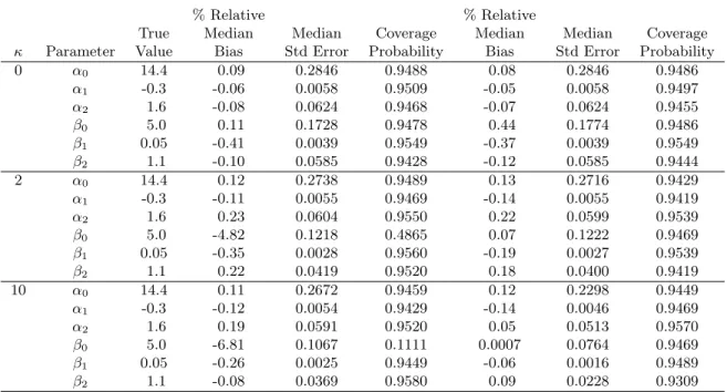
Table 2.1 shows the percent relative bias, median standard error, and coverage probability of each parameter from fitting each sample to both the log-normal and LSN MTP models. The log-normal marginalized model failed to converge 3 times when κ = 0 and once each when κ= 2 andκ= 10; the LSN model failed to converge 46 times when κ= 0, twice when

κ = 2, and once when κ = 10. Likelihood ratio tests favored the LSN model in 3.2% of samples when κ= 0 and in 100% of samples whenκ= 2 or κ= 10.

Under all scenarios, bias remained small and coverage probabilities were approximately 0.95 for all parameters except β0. As skewness increased, bias increased for β0 under the log-normal MTP model, and the coverage probability dropped to as low as 0.11 whenκ= 10. While estimates of the remaining parameters would still be valid regardless of which model were used, when the data are skewed, the log-normal model is not appropriate for making predictions or estimating the overall mean, exp(x0_iβ), due to the bias in β0. Efficiency gains were also observed for the LSN MTP model when skewness was present; standard errors were somewhat smaller under the LSN model than the log-normal model when κ = 2 and even more so when κ = 10. These results indicate that the proposed MTP models provide unbiased estimates of regression coefficients. In the presence of skewness, however, the LSN model should be used to improve efficiency and yield unbiased predictions of the marginal mean, exp(x0_iβ), since this is a function ofβ0.

2.4 Analysis of MOVE! Intervention Data

(45)

VA patients (Kahwati et al. 2011). The high cost of obesity is well documented (Arterburn et al. 2005; Finkelstein et al. 2009), and the MOVE! intervention is the first behavioral weight loss program implemented across an entire health system. MOVE! was implemented as an unfunded mandate, so understanding its effect on average health care expenditures is important to guide program planning and refinement in VA. Assessment of the effect of MOVE! on the marginal mean of the entire VA population is also important for other health care systems that are also considering the adoption of behavioral interventions for reigning in the increasing costs of obesity. We use our marginalized two-part model to provide an estimate of the effect of the MOVE! intervention on the marginal mean expenditures among obese veterans.

The data for this analysis was drawn from a retrospective cohort study of obese VA patients eligible for MOVE! in fiscal years 2006-2009 who were identified from a longitudinal study of the VA cost of obesity. Data were obtained from the VA Corporate Data Warehouse (CDW) and the VA Outpatient Care File (OPC). As a part of a larger study, data were first obtained on all veterans who had received VA services and had a weight measurement in 2002 (N=3,365,004). This sample was then stratified into veterans who ever had one or more MOVE! clinic visits in 2006-2009 (MOVE! enrollees) or veterans who did not have a MOVE! clinic visit in this timeframe (non-enrollees).

Veterans were excluded from both cohorts if they were older than 70 in 2010, had a BMI of less than 30 kg/m2 _{within 30 days of the index date, did not have sex data available,} or had contraindications to MOVE! use during year of MOVE! initiation. Weight loss con-traindications that warranted exclusion were central nervous system infections, organic brain syndromes or dementias, anorexia, anterior horn diseases, Huntington’s disease, cirrhosis, dialysis, emphysema, neurological disorders, hepatitis, recent transplant surgery, or recent cancer treatment. Patients residing in nursing homes, hospice, or residential or adult day health care were also excluded.

(46)

race (white or non-white), marital status (married or non-married), copay status (exempt vs. non-exempt), and veterans integrated service network (VISN) of residence. Then, potential matches were retained on the basis of BMI and comorbidity burden, assessed via the 2002 diagnostic cost group (DCG) score. Only matches with the same integer BMI measure oc-curring within 7 days of baseline measure of their respective MOVE! enrollee and the same DCG score (closest integer) were retained. The final cohort included 18,214 MOVE! enrollees and 18,214 non-enrollees.

The expenditure outcome of interest was total VA expenditures in the fiscal year following MOVE! initiation and was obtained from the VA Health Economics Resource Center. Ex-penditures for non-VA services were excluded as this analysis took a VA payer perspective. Total expenditures were inflation-adjusted to 2011 dollars using the general Consumer Price Index (CPI) because medical CPI does not adequately account for technological improvement, quality change and improved health outcomes (Berndt et al. 2002). The explanatory variable of primary interest was MOVE! initiation, which could occur any time between October 2005 and September 2009.

Descriptive statistics for the covariates and outcome are shown in Table 2.2. Of note, 17% percent of MOVE! enrollees and 14% percent of non-enrollees had zero health care expenditures in the year following initiation, yielding standard one-part log-normal or LSN models inappropriate. To assess the effect of MOVE! enrollment on health care expenditures in the following year, we fit the MTP model:

logit(πi) =α0+α1xi1+α2xi2+α3xi3+α4xi4

E(Yi) = exp(β0+β1xi1+β2xi2+β3xi3+β4xi4)

(47)

and standard errors from the log-normal and LSN MTP models. Table 2.4 presents model-estimated mean expenditures from the LSN model at the quartile values of age, BMI, and DCG score for MOVE! enrollees and non-enrollees.

The estimates from the two models are quite similar, although a likelihood ratio test indicated that the LSN model was the more appropriate fit (p < 0.0001). Both models estimate an odds ratio of exp(−0.24) = 0.79, indicating that the odds of incurring health care expenditures in the fiscal year following MOVE! enrollment were approximately 21% lower for those enrolled in MOVE! compared to non-enrollees with 95% confidence interval [CI] (17%, 26%). Despite the lower probability of incurring expenditures, however, we estimated from the log-normal MTP model that enrollment in MOVE! was associated with exp(0.1749) = 1.19 times higher total health care expenditures on average in the following fiscal year with 95% Wald-type CI (1.16, 1.23). Similarly, the LSN MTP model estimated that MOVE! enrollment was associated with exp(0.1790) = 1.20 times higher total health care expenditures on average in the following fiscal year with 95% CI (1.16, 1.23). While expenditures for non-enrollees remained lower than those of MOVE! enrollees, expenditures for both groups trended upward with increasing BMI and DCG score. Note that the estimated means for MOVE! enrollees at each quartile were 1.20 times higher than those of non-enrollees, reflecting the homogeneous model-estimated treatment effect across the distribution of age, BMI, and DCG score.

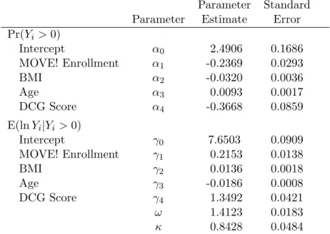
For comparison, we additionally fit the conventional two-part mixture model to these data. Using the same covariates as in the original analyses, we fit a logistic regression model to estimate the probability of incurring positive expenditures among the 36,428 individuals in our cohort and a log-skew-normal model on the subset of 30,847 individuals who had positive expenditures to estimate the level of expenditures conditional on occurrence. Thus, we fit the model:

logit(πi) =α0+α1xi1+α2xi2+α3xi3+α4xi4

(48)

Table 2.5 presents the regression estimates and standard errors from this model. The parameter estimates were similar to those estimated from the MTP model in Table 2.3. This reflects the fact that the percentage of zeros was not large, and hence the marginal mean was primarily driven by the positive expenditure values. Similar to our proposed model, the logistic regression suggested that MOVE! enrollment was associated with 21% lower odds of incurring health care costs in the following fiscal year compared to non-enrollees (95% CI [16%, 26%]). In contrast, the LSN model estimated that, conditional on incurring expenditures, those enrolled in MOVE! had 0.22 higher expenditures on the log scale on average than those not enrolled in MOVE! (p <0.0001). However, with such conflicting results in the binary and continuous parts of this model, investigators are left without a clear sense of the combined overall effect of such an intervention on the average population cost. The MTP model, on the other hand, provides a single, easily interpreted estimate of the overall effect.

These MTP model results suggest that VA expenditures are not reduced in the year follow-ing MOVE! initiation, possibly because few veterans have sustained an intense participation in this behavioral weight loss program (Kahwati et al. 2011). This finding has important im-plications for VA policymakers needing to address the increasing incidence and prevalence of obesity among veterans. In particular, these results suggest that VA may need to introduce alternative weight management strategies to reduce expenditures among obese veterans or increase the effectiveness of MOVE! to induce expenditure reductions. It is possible that vet-erans’ more recent (2012-2014) experience with MOVE! is more sustained and translates into VA expenditure reductions, but these findings suggest that enrollment in MOVE! in its initial four years was not associated with lower VA expenditures in the year following initiation, compared to non-enrollees.

2.5 Conclusion

(49)

account-ing for the excess number of zeros. While log-normal models are most commonly used, we also extended our MTP model to the broader and more flexible log-skew-normal distribution which allows asymmetry and skewness in the data and contains the log-normal distribution as a special case. In our simulation study, the maximum likelihood parameter estimates had near zero bias and good coverage properties in all scenarios except for the intercept from the log-normal model when fit to skewed data. As such, using either the log-normal or LSN MTP model should be reliable for estimating effects of covariates, although additional care should be used when predicting marginal means for specified covariate groups.

Using the LSN MTP model, we estimated that enrollment in the MOVE! weight loss intervention was associated with 20% higher average health care expenditures in the year after MOVE! initiation compared to a control group of non-enrollees. VA policymakers may need to refine the MOVE! program or introduce alternative behavioral weight programs to reduce expenditures among obese veterans. In contrast, the conventional two-part model found that MOVE! enrollment was associated with a decrease in the probability of incurring positive expenditures, but was also associated with an increase in the level of expenditures given they were incurred, leading to conflicting conclusions about the overall effect of the MOVE! program. Future directions for the MTP model could include extensions to clustered or spatially correlated data and applications to other fields, such as substance abuse or psy-chometric research. We are currently working to extend the MTP model to longitudinal data, allowing investigators to examine trends in the marginal mean over time. For example, it is possible that the effect of the MOVE! weight loss intervention may vary after additional years of enrollment, and estimating this effect would have important policy implications.

(50)

Table 2.1: Marginalized two-part model performance with 1,000 simulations and varying skewness

Log-normal model Log-skew-normal model

% Relative % Relative

True Median Median Coverage Median Median Coverage

κ Parameter Value Bias Std Error Probability Bias Std Error Probability 0 α0 14.4 0.09 0.2846 0.9488 0.08 0.2846 0.9486

α1 -0.3 -0.06 0.0058 0.9509 -0.05 0.0058 0.9497 α2 1.6 -0.08 0.0624 0.9468 -0.07 0.0624 0.9455 β0 5.0 0.11 0.1728 0.9478 0.44 0.1774 0.9486 β1 0.05 -0.41 0.0039 0.9549 -0.37 0.0039 0.9549 β2 1.1 -0.10 0.0585 0.9428 -0.12 0.0585 0.9444

2 α0 14.4 0.12 0.2738 0.9489 0.13 0.2716 0.9429 α1 -0.3 -0.11 0.0055 0.9469 -0.14 0.0055 0.9419 α2 1.6 0.23 0.0604 0.9550 0.22 0.0599 0.9539 β0 5.0 -4.82 0.1218 0.4865 0.07 0.1222 0.9469 β1 0.05 -0.35 0.0028 0.9560 -0.19 0.0027 0.9539 β2 1.1 0.22 0.0419 0.9520 0.18 0.0400 0.9419

(51)

Table 2.2: Means (SD) for MOVE! data

MOVE!

Non-Enrollees Enrollees (n=18,214) (n=18,214)

Covariates

Age 61 (9.3) 61 (9.3)

BMI 35.2 (3.9) 35.1 (3.9)

DCG Score 0.24 (0.17) 0.24 (0.17)

Outcomes

% Positive Cost 83.2 86.2

Total Costs 7005 (18866) 6542 (18641)

(52)